Computer simulations of interferometric imaging with the VLT interferometer and the AMBER instrument

Abstract

We present computer simulations of interferometric imaging with the VLT interferometer and the AMBER instrument. These simulations include both the astrophysical modelling of a stellar object by radiative transfer calculations and the simulation of light propagation from the object to the detector (through atmosphere, telescopes, and the AMBER instrument), simulation of photon noise and detector read-out noise, and finally data processing of the interferograms. The results show the dependence of the visibility error bars on the following observational parameters: different seeing during the observation of object and reference star (Fried parameters $r_{0,{\rm object}}$=2.4 m, $r_{0,{\rm ref.}}$=2.5 m), different residual tip-tilt error ($\delta_{\rm tt,object}$=2% of the Airy disk diameter, $\delta_{\rm tt,ref.}$=0.1%), and object brightness ($K_{\rm object}$=3.5 mag and 11 mag, $K_{\rm ref.}$=3.5 mag). Exemplarily, we focus on stars in late stages of stellar evolution and study one of its key objects, the dusty supergiant IRC +10 420 that is rapidly evolving on human timescales. We show computer simulations of VLTI interferometry of IRC +10 420 with two ATs (wide-field mode, i.e. without fiber optics spatial filters) and discuss whether the visibility accuracy is sufficient to distinguish between different theoretical model predictions.

Keywords: VLTI, AMBER, interferometric imaging, IRC +10 420, dust shells, circumstellar matter, supergiants, stellar evolution

1 INTRODUCTION

The Very Large Telescope Interferometer[1] (VLTI) with its four 8.2 m unit telescopes (UTs) and three 1.8 m auxiliary telecopes (ATs) will certainly establish a new era of optical and infrared interferometric imaging within the next few years. With a maximum baseline of up to more than 200 m, the VLTI will allow the study of astrophysical key objects with unprecendented resolution opening up new vistas to a better understanding of their physics.

The near-infrared focal plane instrument of the VLTI, the Astronomical MultiBEam Recombiner[2, 3] (AMBER), will operate between 1 and 2.5 $\mu$m and for up to three beams allowing the measurement of closure phases. In a second phase its wavelength coverage is planned to be extended to 0.6 $\mu$m. Objects as faint as $K=20$ mag are expected to be observable with AMBER when a bright reference star is available, and as faint as $K=14$ mag otherwise.

Among the astrophysical key issues[4] are, for instance, young stellar objects, active galactic nuclei and stars in late phases of stellar evolution. The simulation of a stellar object consists in principle of two components:
(i) the calculation of an astrophysical model of the object, typically based on radiative transfer calculations predicting, e.g., its intensity distribution. To obtain a robust and non-ambiguous model, it is of particular importance to take diverse observational constraints into account, for instance the spectral energy distribution and visibilities.
(ii) the determination of the interferometer’s response to this intensity signal, i.e. the simulation of light propagation in the atmosphere and the interferometer.
Often, only one of the above parts is considered in full detail. The aim of this study is to combine both efforts and to present a computer simulation of the VLTI performance for observations of one object class, the dusty supergiants. For this purpose, we calculated a detailed radiative transfer model for one of its most outstanding representatives, the supergiant IRC +10 420, and carried out computer simulations of VLTI visibility measurements. The goal is to estimate how accurate visibilities can be measured with the VLTI in this particular but not untypical case, to discuss if the accuracy is sufficient to distinguish between different theoretical model predictions and to study on what the accuracy is dependent.

2 The supergiant IRC +10 420: Evolution on human timescales

The star IRC +10 420 (= V 1302 Aql = IRAS 19244+1115) is an outstanding object for the study of stellar evolution. Its spectral type changed from F8 I${}_{\rm a}^{+}$ in 1973[5] to mid-A today[6, 7] corresponding to an effective temperature increase of 1000-2000 K within only 25 yr. It is one of the brightest IRAS objects due to its very strong infrared excess by circumstellar dust and one of the warmest stellar OH maser sources known[8, 9, 10]. Large mass-loss rates, typically of the order of several $10^{-4}$ M_⊙/yr were determined by CO observations[11, 6]. IRC +10 420 is believed to be a massive luminous star currently being observed in its rapid transition from the red supergiant stage to the Wolf-Rayet phase[9, 10, 12, 6, 7]. Its massive nature (initially $\sim 20$ to 40 M_⊙) can be concluded from its distance ($d$ = 3–5 kpc) and large wind velocity (40 km/s) ruling out alternative scenarios. IRC +10 420 is the only object observed until now in its transition to the Wolf-Rayet phase. The structure of the circumstellar environment of IRC +10 420 appears to be very complex[13], and scenarios proposed to explain the observed spectral features of IRC +10 420 include a rotating equatorial disk[12], bipolar outflows[14], and the infall of circumstellar material onto the star’s photosphere [15].

Several infrared speckle and coronographic observations [16, 17, 18, 19, 20] were conducted to study the dust shell of IRC +10 420. The most recent study[21] reports the first diffraction-limited 73 mas bispectrum speckle interferometry of IRC +10 420 and presents the first radiative transfer calculations that model both the spectral energy distribution and the visibility of this key object. In the following we will briefly describe the main results and conclusions of this study which will serve as astrophysical input for the VLTI computer simulations presented in the next section.

2.1 Visibility measurements and bispectrum speckle interferometry

Speckle interferograms of IRC +10 420 were obtained with the Russian 6 m telescope at the Special Astrophysical Observatory on June 13 and 14, 1998[21]. The speckle data were recorded with our NICMOS-3 speckle camera through an interference filter with a centre wavelength of 2.11 $\mu$m and a bandwidth of 0.19 $\mu$m. The observational parameters were as follows: exposure time/frame 50 ms; number of frames 8400; 2.11 $\mu$m seeing (FWHM) $\sim$1$.\!\!^{\prime\prime}$0. A diffraction-limited image of IRC +10 420 with 73 mas resolution was reconstructed from the speckle interferograms using the bispectrum speckle interferometry method[22, 23, 24]. The modulus of the object Fourier transform (visibility) was determined with the speckle interferometry method[25].

Figure 1: Left: Azimuthally averaged 2.11 $\mu$m visibility of IRC +10 420 with error bars for selected frequencies. This visibility function consists of a constant plateau (visibility $\sim 0.6$) caused by the unresolved central object and a triangle-shaped low-frequency function caused by the faint extended nebula. Right: Azimuthally averaged radial plots of the reconstructed diffraction-limited $2.11\mu$m-images of IRC +10 420 (solid line) and HIP 95447 (dashed line).

Figure 1 (left panel) shows the reconstructed 2.11 $\mu$m visibility function of IRC +10 420. There is only marginal evidence for an elliptical visibility shape (position angle of the long axis $\sim 130\hbox{${}^{\circ}$}\pm 20\hbox{${}^{\circ}$}$, axis ratio $\sim 1.0$ to 1.1). The visibility 0.6 at frequencies $>4$ cycles/arcsec shows that the stellar contribution to the total flux is $\sim$ 60% and the dust shell contribution is $\sim$ 40%. The Gauß fit FWHM diameter of the dust shell was determined to be $d_{\rm FWHM}=(219\pm 30)$ mas. By comparison, previous 3.8 m telescope K-band observations[19] found a dust-shell flux contribution of $\sim$50% and $d_{\rm FWHM}=216$ mas. However, as will be shown later, a ring-like intensity distribution appears to be much better suited than the assumption of a Gaussian distribution whose corresponding FWHM diameter fit may give misleading sizes (see Sect. 2.2). The right panel of Fig. 1 displays the azimuthally averaged diffraction-limited images of IRC +10 420 and the unresolved star HIP 95447. The $K$-band visibility will strongly constrain radiative transfer calculations as shown in the next section.

2.2 Dust-shell models

The spectral energy distrubion (SED) of IRC +10 420 with 9.7 and 18 $\mu$m silicate emission features is shown in Fig. 2. It corresponds to the ’1992’ data set used by Oudmaijer et al.[6]) and combines VRI (October 1991), near-infrared (March and April 1992) and Kuiper Airborne Observatory (June 1991) photometry[12] with the IRAS measurements and 1.3 mm data[26]. Additionally, we included data for $\lambda<0.55\,\mu$m[27]. In contrast to the near-infrared, the optical magnitudes have remained constant during the last twenty years within a tolerance of $\approx 0\hbox{$.\!\!^{\rm m}$}1$.

IRC +10 420 is highly reddened due to an extinction of $A^{\rm total}_{\rm V}\approx 7^{\rm m}$ by the interstellar medium and the circumstellar shell. From polarization studies an interstellar extinction of $A_{\rm V}\approx 6^{\rm m}$ to $7^{\rm m}$ was estimated [27, 12]. Based on the strength of the diffuse interstellar bands, $E(B-V)=1\hbox{$.\!\!^{\rm m}$}4\pm 0\hbox{$.\!\!^{\rm m}$}5$ can be inferred for the interstellar contribution compared to a total of $E(B-V)=2\hbox{$.\!\!^{\rm m}$}4$[15]. We will use an interstellar $A_{\rm V}$ of $5^{\rm m}$ adopting the method of Savage & Mathis [28] with $A_{\rm V}=3.1E(B-V)$[6].

Figure 2: SED (top) and 2.11 $\mu$m visibility (bottom) for a superwind model with $Y=r/r_{1}=4.5$ and different amplitudes. The inner shell obeys a $1/r^{2}$ density distribution, the outer shell a $1/r^{1.7}$ density distribution. Model parameters are: black body, $T_{\rm eff}=7000$ K, $T_{1}=1000$ K, $\tau_{0.55\mu{\rm m}}=7.0$, silicates[32], standard grain size distribution[31] with $a_{\rm max}=0.45\,\mu$m, and $Y_{\rm out}=10^{4}$. The symbols refer to the observations (see text) corrected for interstellar extinction of $A_{\rm v}=5^{\rm m}$.

In order to model both the observed SED and $2.11\,\mu$m visibility, we performed radiative transfer calculations for dust shells assuming spherical symmetry. We used the code DUSTY[29] which solves the spherical radiative transfer problem utilizing the self-similarity and scaling behaviour of IR emission from radiatively heated dust[30]. To solve the radiative transfer problem including absorption, emission and scattering several properties of the central source and its surrounding envelope are required, viz. (i) the spectral shape of the central source’s radiation; (ii) the dust properties, i.e. the envelope’s chemical composition and grain size distribution as well as the dust temperature at the inner boundary; (iii) the relative thickness of the envelope, i.e. the ratio of outer to inner shell radius, and the density distribution; and (iv) the total optical depth at a given reference wavelength. The code has been expanded for the calculation of synthetic visibilities.

Figure 3: Left: Fractional contributions of the emerging stellar radiation as well as of the scattered radiation and of the dust emission to the total flux as a function of the wavelength for a superwind model with $Y=r/r_{1}=4.5$, $A=40$ and a $1/r^{1.7}$ density distribution in the outer shell. Model parameters are: black body, $T_{\rm eff}=7000$ K, $T_{1}=1000$ K, $\tau_{0.55\mu{\rm m}}=7.0$, silicates[32], standard grain size distribution[31] with $a_{\rm max}=0.45\,\mu$m, and $Y_{\rm out}=10^{4}$. Right: Corresponding normalized intensity vs. angular displacement $\vartheta$. The (unresolved) central peak belongs to the central star. The inner hot rim of the circumstellar shell has a radius of 35 mas, and the cool component is located at 155 mas. Both loci correspond to local intensity maxima.

We calculated various models of the dust shell of IRC +10 420 considering black bodies and model atmospheres as central sources of radiation, different silicates, grain-size and density distributions. We refer to Blöcker et al. [21] for a full description of the model grid. The remaining fit parameters are the dust temperature, $T_{1}$, which determines the radius of the shell’s inner boundary, $r_{1}$, and the optical depth, $\tau$, at a given reference wavelength, $\lambda_{\rm ref}$. We refer to $\lambda_{\rm ref}=0.55\,\mu$m. Models were calculated for dust temperatures between 400 and 1000 K and optical depths between 1 and 12. Significantly larger values for $\tau$ lead to silicate features in absorption.

The near-infrared visibility strongly constrains dust shell models since it is, e.g., a sensitive indicator of the grain size. Accordingly, high-resolution interferometry results provide essential ingredients for models of circumstellar dust-shells. In the instance of IRC +10 420 (assuming the central star to be a black body of $T_{\rm eff}=7000$ K), the silicate[32] grain sizes, $a$, were found to be in accordance with a standard distribution function[31], $n(a)$ $\sim$ $a^{-3.5}$, with $a$ ranging between $a_{\rm min}$ = 0.005 $\mu$m and $a_{\rm max}$ = 0.45 $\mu$m.

However, the observed dust shell properties cannot be fitted by single-shell models but seem to require multiple components. At a certain distance we considered an enhancement over the assumed $1/r{{}^{x}}$ density distribution. The best model for both SED and visibility was found for a dust shell with a dust temperature of 1000 K at its inner radius of $r_{1}=69\,R_{\ast}$. At a distance of $r=308\,R_{\ast}$ ($Y=r/r_{1}=4.5$) the density was enhanced by a factor of $A=40$ and and its density exponent was changed from $x=2$ to $x=1.7$. These fits for SED and 2.11 $\mu$m visibility are shown in Fig. 2. The various flux contributions at 2.11 $\mu$m are 62.2% stellar light, 26.1% scattered radiation and 10.7% dust emission (see Fig. 3), i.e. the radiation emitted by the circumstellar shell itself consists of 71% scattered radiation and 29% direct dust emission. The shell’s model intensity distribution is shown in Fig. 3 and was found to be ring-like. This appears to be typical for optically thin shells (here $\tau_{0.55\mu{\rm m}}=7$, $\tau_{2.11\mu{\rm m}}=0.55$) showing limb-brightened dust-condensation zones. Accordingly, the interpretation of the observational data by FWHM Gauß diameters may give misleading results. The ring diameter is equal to the inner diameter of the hot shell ($\sim 69$ mas), and the diameter of the central star amounts to $\sim 1$ mas. The bolometric flux, $F_{\rm bol}$, is $8.17\cdot 10^{-10}$ Wm^-2 corresponding to a central-star luminosity of $L/L_{\odot}=25\,462\cdot(d/{\rm kpc})^{2}$.

This two-component model can be interpreted in terms of a termination of an enhanced mass-loss phase roughly 90 yr (for $d=5$ kpc) ago. The assumption that IRC +10 420 had passed through a superwind phase in its recent history is in line with its evolutionary status of an object in transition from the Red-Supergiant to the Wolf-Rayet phase. The mass-loss rates of the components can be determined to be $\dot{M}_{1}=7.0\ 10^{-5}$ $M_{\odot}/{\rm yr}$ and $\dot{M}_{2}=1.1\ 10^{-3}$ $M_{\odot}/{\rm yr}$.

3 Interferometry with the VLTI and the AMBER instrument

In the previous section, the spatial intensity profile of the dusty supergiant IRC +10 420 (see Fig. 3) was derived by means of radiative transfer models and their comparison with photometric and interferometric observations. This $2.11\,\mu$m intensity profile will serve as object intensity profile in the simulation of monochromatic VLTI observations. The next steps are the simulation of light propagation from the object to the detector (through atmosphere, telescopes, and the AMBER wide-field mode instrument), simulation of photon noise and detector read-out noise, and finally data processing of the interferograms. A schematic view of Michelson interferometry with the VLTI and the AMBER camera is given in Fig. 4.

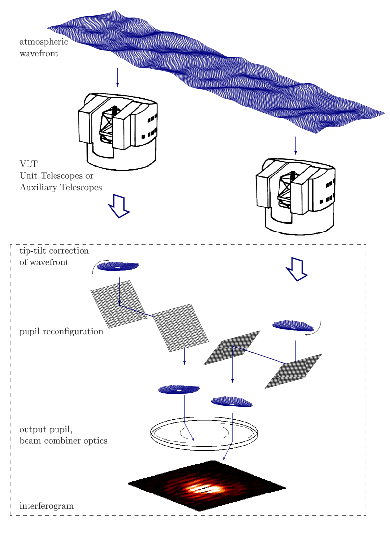
Figure 4: Schematic view of interferometric imaging with the VLTI AMBER camera.

3.1 Computer simulation of interferometric imaging

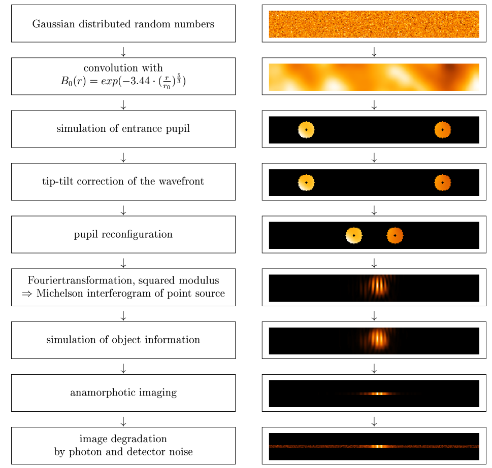
Figure 5: Flow chart of the simulation of VLTI AMBER interferograms (wide-field mode, i.e. without fiber optics spatial filtering).

Fig. 5 shows a flow chart of our simulation of interferometric imaging with the VLTI (ATs, or UTs with adaptive optics) and the AMBER camera in the wide-field mode (i.e. without fiber optics spatial filtering). In a first step, an array of Gaussian distributed random numbers is generated and convolved with the correlation function of the atmospheric refraction index variations in order to generate wavefronts degraded by atmospheric turbulence[33]. The typical size of the atmospheric turbulence cells is given by the Fried parameter $r_{0}$. After the simulation of the entrance pupil, the next step incorporates the tip-tilt correction but we allow for a residual tip-tilt error $\delta_{\rm tt}$. In the next step a typical Michelson output pupil is simulated (pupil reconfiguration). The output pupil is chosen such that (i) in the optical transfer function the off-axis peaks are separated from the central peak, and (ii) the interferograms are sampled with the smallest number of pixels to assure the lowest influence of detector noise. The following step includes light propagation through the beam combiner lens to the focal plane. The squared modulus of the Fourier transform of the complex amplitude in front of the beam combiner lens yields the intensity distribution of a Michelson interferogram of a point source. In the next step the required object intensity distribution is simulated (given here by the intensity distribution of IRC +10 420) to obtain the Michelson interferogram of the object: The Fourier transformation of the object intensity distribution, calculated at those spatial frequencies covered by the the simulated interferometer baseline vector, is multiplied with the off-axis peaks of the transfer function of the generated Michelson interferogram[34]. Finally, Poisson photon-noise and detector read-out noise is injected to the interferograms. The noise level depends, among other parameters, on the number of detectable photons, the total optical throughput of the interferometer and the quantum efficiency of the detector. Details[35] are shown in Table 1.

Table 1: Parameters of simulations

wavelength	brightness	opt. throughput	read-out noise	quantum efficiency	exposure	photon number
$2.11\,\mu$m	$K=3.5$ mag	0.108	15 e-	0.6	50 ms	$4.42\cdot 10^{6}$

3.2 Visibility data for IRC +10 420

We performed simulations of IRC +10 420 AT visibility observations in the AMBER wide-field mode and studied the influence of various observational parameters on the visibility accuracy. Visibility error bars were, for example, obtained for the following observational parameters: different seeing during the observation of object and reference star (Fried parameters $r_{0,{\rm object}}$=2.4 m, $r_{0,{\rm ref.}}$=2.5 m), different residual tip-tilt error ($\delta_{\rm tt,object}$=2% of the Airy disk diameter, $\delta_{\rm tt,ref.}$=0.1%), and object brightness ($K_{\rm object}$=3.5 mag and 11 mag, $K_{\rm ref.}$=3.5 mag). In the computer experiments (a)-(c), object and reference star were assumed to have the same brightness ($K$=3.5 mag, see Table 1), in experiment (d) fainter objects ($K$=11 mag) were simulated as well. Fig. 6 shows the results of the simulations (a) to (c) based on the $A=40$ intensity profile (see Fig. 3) for baselines of 50 and 100 m together with the model predictions for IRC +10 420. To obtain error bars each simulation was repeated three times. The insetted table lists the parameters of the simulations.

Simulation (a) based on 2400 interferograms represents the ideal case of excellent seeing conditions ($r_{0,{\rm object}}$=2.5 m, $r_{0,{\rm ref.}}$=2.5 m) and an almost perfect tip-tilt correction (residual tip-tilt error $\delta_{\rm tt}=0.1$%). The visibility error $\Delta V$ amounts to $\pm 0.0029$. Simulation (b) illustrates the influence of a larger residual object tip-tilt error ($\delta_{\rm tt}$=2%) leading to $\Delta V\pm 0.0036$. Simulation (c) shows the impact of different seeing conditions for object and reference star. In the last simulation (d) of this series (shown only in the insetted table of Fig. 6) an IRC +10 420-like intensity distribution is assumed but the simulated $K$-magnitude is 11 mag (instead of 3.5 mag). Although the photon number decreases to $N=4.41\cdot 10^{3}$ (i.e. by a factor of 1000, see Table 1), the visibility accuracy is still high, i.e. $\Delta V\pm 0.0036$.

Figure 6: Dependence of the error bars of simulated AT-VLTI/AMBER (wide-field mode) observations of IRC +10 420 at 2.11 $\mu$m on (i) seeing differences of object and reference star observations (Fried parameter, $r_{0}$, differences); (ii) different residual tip-tilt errors, $\delta_{\rm tt}$, of object and reference star observations; and (iii) object brightness. Lines refer to radiative transfer models of different superwind amplitudes $A$. The symbols refer to AT-VLTI/AMBER simulations (each with $N$=2400 interferograms) of the $A$=40 intensity profile (see Fig. 3) for baselines of 50 and 100 m (100 m: $q$=227 arc sec^-1). To better distinguish between the simulations, the data points belonging to one baseline are somewhat shifted with respect to the spatial frequency. The error bars are based on a triple iteration of each simulation. The table gives the parameters of the simulations (a) to (d). Note that though simulation (d) corresponds to an IRC +10 420-like intensity distribution, it refers to a much fainter object of $K$=11 mag (instead of 3.5 mag).

	(a)		(b)		(c)		(d)
	obj	ref	obj	ref	obj	ref	obj	ref
$K$-mag.	3.5	3.5	3.5	3.5	3.5	3.5	11	3.5
$r_{0}$	2.5	2.5	2.5	2.5	2.4	2.5	2.5	2.5
$\delta_{\rm tt}$	0.1%	0.1%	2.0%	0.1%	0.1%	0.1%	0.1%	0.1%
$N$	2400	2400	2400	2400	2400	2400	2400	2400
$\Delta V$	$\pm 0.0029$		$\pm 0.0036$		$\pm 0.0064$		$\pm 0.0036$

4 Conclusions

We have presented computer simulations of interferometric imaging with the VLT interferometer and the AMBER instrument in the wide-field mode. These simulations include both the astrophysical modelling of a stellar object by radiative transfer calculations and the simulation of light propagation from the object to the detector and simulation of photon noise and detector read-out noise. We focussed on stars in late stages of stellar evolution and examplarily studied one of its most outstanding representatives, the dusty supergiant IRC +10 420. The model intensity distribution of this key object, obtained by radiative transfer calculations, served as astrophyiscal input for the VLTI/AMBER simulations.

The results of these simulations show the dependence of the visibility error bar on various observational parameters. With these simulations at hand one can immediately see under which conditions the visibility data quality would allow us to discriminate between different model assumptions (e.g. the size of the superwind amplitude). Inspection of Fig. 6 shows that in all studied cases the observations will give clear preference to one particular model. Therefore, observations with VLTI will certainly be well suited to gain deeper insight into the physics of dusty supergiants.

References

- [1] Glindemann, A., et al., 2000, Proc. SPIE Conf. 4006-01
- [2] Petrov, R., Malbet, F., Richichi, A., Hofmann, K.-H.: 1998, ESO Messenger 92, 11
- [3] Petrov, R., et al. , 2000, Proc. SPIE Conf. 4006-07
- [4] Richichi, A., et al., 2000, Proc. SPIE Conf. 4006-08
- [5] Humphreys R.M., Strecker D.W., Murdock T.L., Low, F.J., 1973, ApJ 179, L49
- [6] Oudmaijer R.D., Groenewegen M.A.T., Matthews H.E., Blommaert J.A.D.L, Sahu K.C., 1996, MNRAS 280, 1062
- [7] Klochkova V.G., Chentsov E.L., Panchuk ,V.E., 1997, MNRAS 292,19
- [8] Giguere P.T., Woolf N.J., Webber J.C., 1976, ApJ 207, L195
- [9] Mutel R.L., Fix J.D., Benson J.M., Webber J.C., 1979, ApJ 228, 771
- [10] Nedoluha G.E., Bowers P.F., 1992, ApJ 392, 249
- [11] Knapp G.R., Morris M., 1985, ApJ 292, 640
- [12] Jones T.J., Humphreys R.M, Gehrz, R.D. et al., 1993, ApJ 411, 323
- [13] Humphreys R.M., Smith N., Davidson K. et al., 1997, AJ 114, 2778
- [14] Oudmaijer R.D., Geballe T.R., Waters, L.B.F.M, Sahu K.C., 1994, A&A 281, L33
- [15] Oudmaijer R.D., 1998, A&AS 129, 541
- [16] Dyck H., Zuckerman B., Leinert C., Beckwith S., 1984, ApJ 287, 801
- [17] Ridgway S.T., Joyce R.R., Connors D., Pipher J.L., Dainty C., 1986, ApJ 302, 662
- [18] Cobb M.L., Fix J.D., 1987, ApJ 315, 325
- [19] Christou J.C., Ridgway S.T., Buscher D.F., Haniff C.A., McCarthy Jr. D.W., 1990, Astrophysics with infrared arrays, R. Elston (ed.), ASP conf. series 14, p. 133
- [20] Kastner J., Weintraub D.A., 1995, ApJ 452, 833
- [21] Blöcker T., Balega Y., Hofmann K.-H., Lichtenthäler J., Osterbart R., Weigelt G., 1999, A&A 348, 805
- [22] Weigelt G., 1977, Optics Commun. 21, 55
- [23] Lohmann A.W., Weigelt G., Wirnitzer B., 1983, Appl. Opt. 22, 4028
- [24] Hofmann K.-H., Weigelt G., 1986, A&A 167, L15
- [25] Labeyrie A., 1970, A&A 6, 85
- [26] Walmsley C.M., Chini R., Kreysa E. et al., 1991, A&A 248, 555
- [27] Craine E.R., Schuster W.J., Tapia S., Vrba F.J., 1976, ApJ 205, 802
- [28] Savage B.D., Mathis J.S., 1979, ARA&A 17, 73
- [29] Ivezić Ž., Nenkova M. Elitzur M., 1997, User Manual for DUSTY, University of Kentucky (http://www.pa.uky.edu/m̃oshe/dusty)
- [30] Ivezić Ž., Elitzur M., 1997, MNRAS 287, 799
- [31] Mathis J.S., Rumpl W., Nordsieck K.H., 1977, ApJ 217, 425
- [32] Draine B.T., Lee H.M., 1984, ApJ 285, 89
- [33] Roddier F., 1981, Progress in Optics XIX, 281
- [34] Tallon M., Tallon-Bosc I., 1992, A&A 253, 641
- [35] Malbet F., et al., 2000, VLTI AMBER Instrument Analysis Review.