The black hole in IC 1459
from HST observations of the ionized gas disk

Abstract

The peculiar elliptical galaxy IC 1459 ($M_{V}=-21.19$, $D=16.5h^{-1}\>{\rm Mpc}$) has a fast counterrotating stellar core, stellar shells and ripples, a blue nuclear point source and strong radio core emission. We present results of a detailed HST study of IC 1459, and in particular its central gas disk, aimed a constraining the central mass distribution. We obtained WFPC2 narrow-band imaging centered on the H$\alpha$+[NII] emission lines to determine the flux distribution of the gas emission at small radii, and we obtained FOS spectra at six aperture positions along the major axis to sample the gas kinematics. We construct dynamical models for the H$\alpha$+[NII] and H$\beta$ kinematics that include a supermassive black hole, and in which the stellar mass distribution is constrained by the observed surface brightness distribution and ground-based stellar kinematics. In one set of models we assume that the gas rotates on circular orbits in an infinitesimally thin disk. Such models adequately reproduce the observed gas fluxes and kinematics. The steepness of the observed rotation velocity gradient implies that a black hole must be present. There are some differences between the fluxes and kinematics for the various line species that we observe in the wavelength range 4569 Å to 6819 Å. Species with higher critical densities generally have a flux distribution that is more concentrated towards the nucleus, and have observed velocities that are higher. This can be attributed qualitatively to the presence of the black hole. There is some evidence that the gas in the central few arcsec has a certain amount of asymmetric drift, and we therefore construct alternative models in which the gas resides in collisionless cloudlets that move isotropically. All models are consistent with a black hole mass in the range $M_{\bullet}=1$—$4\times 10^{8}\>{\rm M_{\odot}}$, and models without a black hole are always ruled out at high confidence. The implied ratio of black holes mass to galaxy mass is in the range $0.4$–$1.5\times 10^{-3}$, which is not inconsistent with results obtained for other galaxies. These results for the peculiar galaxy IC 1459 and its black hole add an interesting data point for studies on the nature of galactic nuclei.

1 Introduction

Supermassive central black holes (BH) have now been discovered in more than a dozen nearby galaxies (e.g., Kormendy & Richstone 1995; Ford et al. 1998; Ho 1998; Richstone 1998, and van der Marel 1999a for recent reviews). BHs in quiescent galaxies were mainly found using stellar kinematics while the BHs in active galaxies were detected through the kinematics of central gas disks. Other techniques deployed are VLBI observations of water masers (e.g., Miyoshi et al. 1995) and the measurement of stellar proper motions in our own Galaxy (Genzel et al. 1997; Ghez et al. 1998). The BH masses measured in active galaxies are all larger than a few times $10^{8}\>{\rm M_{\odot}}$, while the BH masses in quiescent galaxies are often smaller. The number of accurately measured BHs is expected to increase rapidly in the near future, especially through the use of STIS on board HST. This will establish the BH ‘demography’ in nearby galaxies, yielding BH masses as function of host galaxy properties. In this respect two correlations in particular have been suggested in recent years. First, a correlation between BH mass and host galaxy (spheroid) optical luminosity (or mass) was noted (e.g., Kormendy & Richstone 1995; Magorrian et al. 1998; van der Marel 1999b). However, this correlation shows considerable scatter (a factor $\sim 10$ in BH mass at fixed luminosity). The scatter might be influenced by selection effects (e.g., it is difficult to detect a low mass BH in a luminous galaxy) and differences in the dynamical modeling. Second, a correlation between BH mass and either core or total radio power of the host galaxy was proposed (Franceschini, Vercellone, & Fabian 1998). However, the available sample is still small and incomplete. Establishing the BH masses for a large range of optical and radio luminosities is crucial to determine the nature of galactic nuclei. An accurate knowledge of BH demography will put constraints on the connection between BH and host galaxy formation and evolution and the frequency and duration of activity in galaxies harboring BHs.

In this paper we measure the BH mass of IC 1459. IC 1459 is an E3 giant elliptical galaxy and member of a loose group of otherwise spiral galaxies. It is at a distance of $16.5h^{-1}\>{\rm Mpc}$ with $M_{V}=-21.19$ (Faber et al. 1989). Williams & Schwarzschild (1979) noted twists in the outer optical stellar isophotes. Stellar spiral ‘arms’ outside the luminous stellar part of the galaxy were detected in deep photographs (Malin 1985). Several stellar shells at tens of kpc from the center were discovered by Forbes & Reitzel (1995). A remarkable feature is the counter-rotating stellar core (Franx & Illingworth 1988) with a maximum rotation of $\sim 170\>{\rm km}\,{\rm s}^{-1}$. IC 1459 also has an extended emission gas disk (diameter $\sim 100^{\prime\prime}$) with spiral arms (Forbes et al. 1990, Goudfrooij et al. 1990) aligned with the galaxy major axis. The disk rotates in the same direction as the outer part of the galaxy (Franx & Illingworth 1988). The nuclear region of IC 1459 has line ratios typical of the LINER class (see e.g., Heckman 1980, Osterbrock 1989 for the definition of LINERS). A warped dust lane is also present. It is misaligned by $\sim 15^{\circ}$ from the galaxy major axis and some dust patches are observed at a radius of $2^{\prime\prime}$ (Carollo et al. 1997). IC 1459 has a blue nuclear optical source with $V=18.3$ (Carollo et al. 1997; Forbes et al. 1995) which is unresolved by HST. It also has a variable compact radio core (Slee et al. 1994). There is no evidence for a radio-jet down to a scale of $1^{\prime\prime}$ (Sadler et al. 1989). IC 1459 has a hard X-ray component, with properties typical of low-luminosity AGNs (Matsumoto et al. 1997).

Given the abovementioned properties, IC 1459 might best be described as a galaxy in between the classes of active and quiescent galaxies. This makes it an interesting object for extending our knowledge of BH demography, in particular since there are only few other galaxies similar to IC 1459 for which an accurate BH mass determination is available. We therefore made IC 1459, and in particular its central gas disk, the subject of a detailed study with the Hubble Space Telescope (HST). We observed the emission gas of IC 1459 with the Second Wide Field and Planetary Camera (WFPC2) through a narrow-band filter around H$\alpha$+[NII] and took spectra with the Faint Object Spectrograph (FOS) at six locations in the inner $1^{\prime\prime}$ of the disk. In Section 2 we discuss the WFPC2 observations and data reduction. In Section 3 we describe the FOS observations and data reduction, and we present the inferred gas kinematics. To interpret the data we construct detailed dynamical models for the kinematics of the H$\beta$ and H$\alpha$+[NII] emission lines in Section 4, which imply the presence of a central BH with mass in the range $1$—$4\times 10^{8}\>{\rm M_{\odot}}$. In Section 5 we discuss how the kinematics of other emission line species differ from those for H$\beta$ and H$\alpha$+[NII], and what this tells us about the central structure of IC 1459. In Section 6 we present dynamical models for ground-based stellar kinematical data of IC 1459, for comparison to the results inferred from the HST data. We summarize and discuss our findings in Section 7.

We adopt $H_{0}=80\>{\rm km}\,{\rm s}^{-1}\>{\rm Mpc}^{-1}$ throughout this paper. This does not directly influence the data-model comparison for any of our models, but does set the length, mass and luminosity scales of the models in physical units. Specifically, distances, lengths and masses scale as $H_{0}^{-1}$, while mass-to-light ratios scale as $H_{0}$.

2 Imaging

2.1 WFPC2 Setup and Data Reduction

We observed IC 1459 in the context of HST program GO-6537. We used the WFPC2 instrument (described in, e.g., Biretta et al. 1996) on September 20, 1996 to obtain images in two narrow-band filters. The observing log is presented in Table 1. The ‘Linear Ramp Filters’ (LRFs) of the WFPC2 are filters with a central wavelength that varies as a function of position on the detector. The LRF FR680P15 was used as ‘on band’ filter, with the galaxy position chosen so as to center the filter transmission on the H$\alpha$+[NII] emission lines. The narrow-band filter F631N was chosen as ‘off-band’ filter, and covers primarily stellar continuum. The position of the galaxy on the chip in the off-band observations was chosen to be the same as in the on-band observations. In all images the galaxy center was positioned on the PC chip, yielding a scale of $0.0455^{\prime\prime}$/pixel.

The images were calibrated with the standard WFPC2 ‘pipeline’, using the most up to date calibration files. This reduction includes bias subtraction, dark current subtraction and flat-fielding. A flatfield was not available for the LRF filter, so we used the flatfield of F658N, a narrow-band filter with similar central wavelength (6590 Å). Three back to back exposures were taken through each filter. In each case, the third exposure was offset by (2,2) PC pixels to facilitate bad pixel removal. The alignment of the exposures (after correction for intentional offsets) was measured using both foreground stars and the galaxy itself, and was found to be adequate. For each filter we combined the three available images without additional shifts, but with removal of cosmic rays, bad pixels and hot pixels.

Construction of a H$\alpha$+[NII] emission image requires subtraction of the stellar continuum from the on-band image. To this end we first fitted isophotes to estimate the ratio of the stellar continuum flux in the on-band and off-band image. This ratio could be fitted as a slowly varying linear function of radius in regions with no emission flux. The off-band image was multiplied by this ratio and subtracted from the on-band image. The resulting H$\alpha$+[NII] emission image was calibrated to units of $\>{\rm erg}\,{\rm s}^{-1}\,{\rm cm}^{-2}$ using calculations with the STSDAS/SYNPHOT package in IRAF. The resulting flux scale was found to be in agreement with that inferred from our FOS spectra (see Section 3).

2.2 The Ionized Gas Disk

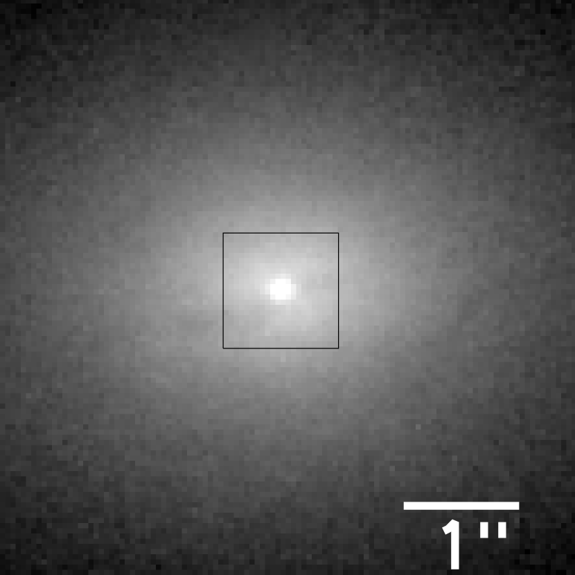
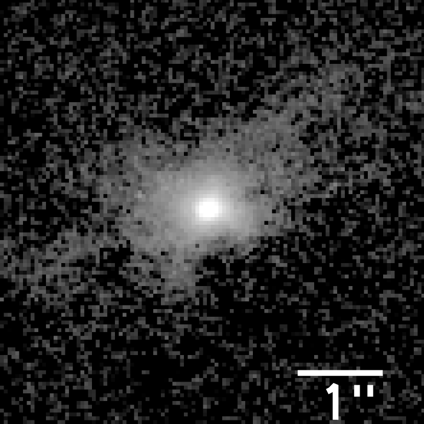
Figure 1: (Left): Stellar continuum image of the central $5^{\prime\prime}\times 5^{\prime\prime}$ of IC 1459. The image was obtained through a narrow-band filter, F631N, which at the redshift of IC 1459 measures primarily stellar continuum. The image was rotated such that the galaxy major axis runs horizontal. A small dust lane runs across the central region. The location of the FOS apertures inside the $1^{\prime\prime}\times 1^{\prime\prime}$ box drawn at the center of the image is shown in Fig. 3. (Right): H$\alpha$+[NII] emission image, at the same scale and orientation. There is a disk of gas with an irregular morphology at $r\gtrsim 0.5^{\prime\prime}$, with filaments extending in various directions.

Figure 1 shows both the F631N stellar continuum image of the central region of IC1459, as well as the H$\alpha$+[NII] image. The continuum image shows a weakly obscuring warped dust lane across the center which is barely visible in the emission image. This dust lane is evident even more clearly in a $V-I$ image of IC 1459 (Carollo et al. 1997). The lane makes an angle of $\sim 15^{\circ}$ with the stellar major axis.

The H$\alpha$+[NII] emission image shows the presence of a gas disk. The existence of this disk was already known from ground-based imaging, which showed that it has a total linear extent of $\sim 100^{\prime\prime}$ (Goudfrooij et al. 1990; Forbes et al. 1990). The outer parts of the disk show weak spiral structure and dust patches. Inside the central $10^{\prime\prime}$ the disk has a somewhat irregular non-elliptical distribution, with filaments extending in various directions. Our HST image shows that the distribution becomes more regular again in the central $r\lesssim 0.5^{\prime\prime}$. Throughout its radial extent, the position angle (PA) of the disk coincides with the PA of the stellar distribution. In the case of the central $0.5^{\prime\prime}$, we derive from isophotal fits ${\rm PA}\approx 37^{\circ}$ for the gas disk. This agrees roughly with the PA of the major axis of the stellar continuum in the same region, for which the F631N image yields ${\rm PA}\approx 34^{\circ}$. Assuming an intrinsically circular disk, Forbes & Reitzel (1995) infer from the ellipticity $\epsilon=0.5$ of the gas disk at several arcseconds an inclination of $60^{\circ}$. We performed a fit to the contour levels of the extended gas emission published by Goudfrooij et al. (1994), which also yields an inclination of $60^{\circ}$. By contrast, the gas distribution in the central $0.5^{\prime\prime}$ of the HST image is rounder than that at large radii. The ellipticity increases from $\epsilon=0.37$ at $r=1.0^{\prime\prime}$ to $\epsilon=0.17$ at $r=0.25^{\prime\prime}$ (approximately the smallest radius at which the ellipticity is not appreciably influenced by the HST point spread function (PSF)). While this could possibly indicate a change in the inclination angle of the disk, it appears more likely that the gas disk becomes thicker towards the center. This latter interpretation receives support from an analysis of the gas kinematics, as we will discuss below (see Section 4.4). In the following we therefore assume an inclination angle of $60^{\circ}$ for IC 1459, as suggested by the ellipticity of the gas disk at large radii.

2.3 The Stellar Luminosity Density

For the purpose of dynamical modeling we need a model for the stellar mass density of IC 1459. Carollo et al. (1997) obtained a HST/WFPC2 F814W (i.e., $I$-band) image of IC 1459, and from isophotal fits they determined the surface brightness profile reproduced in Figure 2. Carollo et al. corrected their data approximately for the effects of dust obscuration through use of the observed $V-I$ color distribution, so dust is not an important factor in the following analysis. To fit the observed surface brightness profile we adopt a parameterization for the three-dimensional stellar luminosity density $j$. We assume that $j$ is oblate axisymmetric, that the isoluminosity spheroids have constant flattening $q$ as a function of radius, and that $j$ can be parameterized as

$$j(R,z)=j_{0}(m/a)^{\alpha}[1+(m/a)^{2}]^{\beta},\quad m^{2}\equiv R^{2}+z^{2}q^{-2}.$$ (1)

Here $(R,z)$ are the usual cylindrical coordinates, and $\alpha$, $\beta$, $a$ and $j_{0}$ are free parameters. When viewed at inclination angle $i$, the projected intensity contours are aligned concentric ellipses with axial ratio $q^{\prime}$, with $q^{\prime 2}\equiv\cos^{2}i+q^{2}\sin^{2}i$. The projected intensity for the luminosity density $j$ is evaluated numerically.

In the following we adopt $i=60^{\circ}$, based on the discussion in Section 2.2. We take $q^{\prime}=0.74$ based on the isophotal shape analysis of Carollo et al. (their figure 1o), which shows an ellipticity $\epsilon$ of $0.26$ in the inner $10^{\prime\prime}$ with variations $<0.05$. The isophotal PA is almost constant, with a monotonic increase of $\sim 5^{\circ}$ between $1^{\prime\prime}$ and $10^{\prime\prime}$. The Carollo et al. results show larger variations in $\epsilon$ and PA in the inner $1^{\prime\prime}$, but these are probably due to the residual effects of dust obscuration. Our model with constant $\epsilon$ and PA is therefore expected to be adequate in the present context. The projected intensity of the model was fit to the observed surface brightness profile between $0.15^{\prime\prime}$ and $5^{\prime\prime}$. The best fit model has $\alpha=-0.62$, $\beta=-0.76$, $a=0.90^{\prime\prime}$ and $j_{0}=1.9\times 10^{2}\>{\rm L_{\odot}}\>{\rm pc}^{-3}$. Its predictions are shown by the solid curve in Figure 2.

The fit was restricted to the range $R\leq 5^{\prime\prime}$. As a result, the fit is somewhat poor at larger radii. This can of course be improved by extending the fit range, but with the simple parametrization of equation (1) this would have led to a poorer fit in the region $R\leq 1^{\prime\prime}$. Since this is the region of primary interest in the context of our spectroscopic HST data (described below), we chose to accept the fit shown in the figure. The central $0.15^{\prime\prime}$ were excluded from the fit because IC 1459 has a nuclear point source. This point source has a blue $V-I$ color. It is most likely of non-thermal origin (similar to the point source in M87; Kormendy 1992; van der Marel 1994) and associated with the core radio emission in IC 1459. If so, the point source does not contribute to the mass density of the galaxy (which is what we are interested in here), and it is therefore appropriate to exclude it from consideration. In Section 7 we briefly discuss the implications of the alternative possibility that the point source is a cluster of young stars.

3 Spectroscopy

3.1 FOS Setup and Data Reduction

We used the red side detector of the FOS (described in, e.g., Keyes et al. 1995) on November 30, 1996 to obtain spectra of IC 1459. The COSTAR optics corrected the spherical aberration of the HST primary mirror. The observations started with a ‘peak-up’ target acquisition on the galaxy nucleus. The sequence of peak-up stages was similar to that described in van der Marel, de Zeeuw & Rix (1997) and van der Marel & van den Bosch (1998; hereafter vdMB98). We then obtained six spectra, three with the 0.1-PAIR square aperture (nominal size, $0.086^{\prime\prime}$) and three with the 0.25-PAIR square aperture (nominal size, $0.215^{\prime\prime}$). The G570H grating was used in ‘quarter-stepping’ mode, yielding spectra with 2064 pixels covering the wavelength range from 4569 Å to 6819 Å. Periods of Earth occultation were used to obtain wavelength calibration spectra of the internal arc lamp. At the end of the observations FOS was used in a special mode to obtain an image of the central part of IC 1459, to verify the telescope pointing.

Galaxy spectra were obtained on the nucleus and along the major axis. A log of the observations is provided in Table 2. Target acquisition uncertainties and other possible systematic effects caused the aperture positions on the galaxy to differ slightly from those commanded to the telescope. We determined the actual aperture positions from the data themselves, using the independent constraints provided by the target acquisition data, the FOS image, and the ratios of the continuum and emission-line fluxes observed through different apertures. This analysis was similar to that described in Appendix A of vdMB98. The inferred aperture positions are listed in Table 2, and are accurate to $\sim 0.02^{\prime\prime}$ in each coordinate. The roll angle of the telescope during the observations was such that the sides of the apertures made angles of $39^{\circ}$ and $129^{\circ}$ with respect to the galaxy major axis. Figure 3 shows a schematic drawing of the aperture positions. Henceforth we use the labels ‘S1’–‘S3’ for the small aperture observations, and ‘L1’–‘L3’ for the large aperture observations.

Most of the necessary data reduction steps were performed by the HST calibration pipeline, including flat-fielding and absolute sensitivity calibration. We did our own wavelength calibration using the arc lamp spectra obtained in each orbit, following the procedure described in van der Marel (1997). The relative accuracy (between different observations) of the resulting wavelength scale is $\sim 0.04$Å ($\sim\!2\>{\rm km}\,{\rm s}^{-1}$). Uncertainties in the absolute wavelength scale are larger, $\sim\!0.4$Å ($\sim\!20\>{\rm km}\,{\rm s}^{-1}$), but influence only the systemic velocity of IC 1459, not the inferred BH mass.

3.2 Gas Kinematics

The spectra show several emission lines, of which the following have a sufficiently high signal-to-noise ratio ($S/N$) for a kinematical analysis: H$\beta$ at 4861 Å; the [OIII] doublet at 4959, 5007 Å; the [OI] doublet at 6300, 6364 Å; the H$\alpha$+[NII] complex at 6548, 6563, 6583 Å; and the [SII] doublet at 6716, 6731 Å. To quantify the gas kinematics we fitted the spectra under the assumption that each emission line is a Gaussian. This yields for each line the total flux, the mean velocity $V$ and the velocity dispersion $\sigma$. For doublets we fitted both lines simultaneously under the assumption that the individual lines have the same $V$ and $\sigma$. The H$\alpha$+[NII] complex is influenced by blending of the lines, and for this complex we made the additional assumptions that H$\alpha$ and the [NII] doublet have the same kinematics, and for the [NII] doublet that the ratio of the fluxes of the individual lines equals the ratio of their transition probabilities (i.e., 3).

Figure 4 shows the observed spectra for each of the five line complexes listed above, with the Gaussian fits overplotted. The figure shows that the observed emission lines are not generally perfectly fit by Gaussians; they often have a narrower core and broader wings. It was shown in vdMB98 that this arises naturally in dynamical models such as those constructed below. In the present paper we will not revisit the issue of line shapes, but restrict ourselves to Gaussian fits (both for the data and for our models). The mean and dispersion of the best-fitting Gaussian are well-defined and meaningful kinematical quantities, even if the lines themselves are not Gaussians.

The Gaussian fit parameters for each of the line complexes are listed in Table 3. The listed velocities are measured with respect to the systemic velocity of IC 1459. The systemic velocity was estimated from the HST data themselves, by including it as a free parameter in the dynamical models described below (see Section 4.2). This yields $v_{\rm sys}=1783\pm 10\>{\rm km}\,{\rm s}^{-1}$ (but with the possibility of an additional systematic error due to uncertainties in the FOS absolute wavelength calibration). This result is a bit higher than values previously reported in the literature (e.g., $v_{\rm sys}=1707\pm 40\>{\rm km}\,{\rm s}^{-1}$ by Sadler 1984; $v_{\rm sys}=1720\>{\rm km}\,{\rm s}^{-1}$ by Franx & Illingworth 1988; $v_{\rm sys}=1748\pm 42\>{\rm km}\,{\rm s}^{-1}$ by Da Costa et al. 1991). In fact, systemic velocities that are up to $150\>{\rm km}\,{\rm s}^{-1}$ smaller than our value have been reported as well (e.g., Davies et al. 1987; Drinkwater et al. 1997).

Figure 5 shows the inferred kinematical quantities for the five line complexes as function of major axis distance. The observational setup provides only sparse sampling along the major axis and with apertures of different sizes, but nonetheless, two items are clear. First, for all apertures and line species there is a steep positive mean velocity gradient across the nucleus (i.e., between observations S1 and S2, or L1 and L2). Second, the velocity dispersion tends to be highest for the smallest aperture closest to the nucleus (observation S1); this is true for all line species with the exception of [SII], for which the dispersion peaks for observation S2. The steep central velocity gradient and centrally peaked velocity dispersion profile are similar to what has been found for other galaxies with nuclear gas disks (e.g., Ferrarese, Ford & Jaffe, 1996; Macchetto et al. 1997; Bower et al. 1998; vdMB98).

The kinematical properties of the different emission line species show both significant similarities and differences. For example, the kinematics of H$\beta$ and H$\alpha$+[NII] are in excellent quantitative agreement. By contrast, [OIII] shows a significantly steeper central mean velocity gradient, and both [OIII] and [OI] have a higher velocity dispersion for several apertures; the central velocity dispersion for [OIII] exceeds that for H$\beta$ and H$\alpha$+[NII] by more than a factor two. The kinematics of the [SII] emission lines deviates somewhat from that for H$\beta$ and H$\alpha$+[NII], but only for the small apertures. There is no a priori reason to expect identical flux distributions, and hence identical kinematics for the different species, because they differ in their atomic structure, ionization potential, critical density, etc. Differences of similar magnitude have been detected in the kinematics of other gas disks as well (e.g., Harms et al. 1994; Ferrarese, Ford & Jaffe 1996). The former authors studied the gas disk in M87, and also found that the [OIII] line indicates a larger mean velocity gradient and higher dispersion than H$\beta$ and H$\alpha$+[NII]. We discuss the differences in the kinematics of the different line species in Section 5, after first having analyzed in detail the kinematics of H$\beta$ and H$\alpha$+[NII] in Section 4.

3.3 Ground-based Spectroscopy

In our modeling it proved useful to complement the FOS spectroscopy with ground-based data that extends to larger radii. We therefore reanalyzed a major axis long-slit spectrum of IC 1459 obtained at the CTIO 4m telescope. The data were taken with a $1.5^{\prime\prime}$-wide slit using a CCD with $0.73^{\prime\prime}$ pixels, in seeing conditions with FWHM $\sim 1.9^{\prime\prime}$. The spectra have a smaller spectral range than the FOS spectra, but do cover the emission lines of H$\beta$ and [OIII]. Fluxes and kinematics for these lines were derived using single Gaussian fits, as for the FOS spectra. The inferred gas kinematics are listed in Table 4. The stellar kinematics implied by the absorption lines in the same spectrum (presented previously by van der Marel & Franx 1993) are used in Section 6 for the construction of stellar dynamical models.

4 Modeling and Interpretation of the H$\alpha$+[NII] and H$\beta$ Kinematics

The FOS spectra of the H$\alpha$+[NII] and H$\beta$ lines yield similar relative fluxes (cf. Figure 6 below) and similar mean velocities and dispersions (cf. Figure 5). We therefore assume that these emission lines have the same intrinsic flux distributions and kinematics. We start in Sections 4.1–4.4 with the construction of models for the H$\beta$ and H$\alpha$+[NII] gas kinematics in which the gas disk is assumed to be an infinitesimally thin structure in the equatorial plane of the galaxy. However, as discussed in Section 2.2, this assumption may not be entirely appropriate at small radii, where the projected isophotes of the gas disk become rounder. In Section 4.5 we therefore discuss models in which the gas distribution is extended vertically.

4.1 Flux Distribution

To model the H$\beta$ and H$\alpha$+[NII] gas kinematics we need a description of the intrinsic (i.e., the deconvolved and de-inclined) flux profile for these emission lines. We model the (face-on) intrinsic flux distribution as a triple exponential,

$$F(R)=F_{1}\exp(-R/R_{1})+F_{2}\exp(-R/R_{2})+F_{3}\exp(-R/R_{3}),$$ (2)

and assume that the disk is infinitesimally thin and viewed at an inclination $i=60^{\circ}$, (cf. Section 2.2). The total flux contributed by each of the three exponential components is $I_{i}=2\pi R_{i}^{2}F_{i}$ ($i=1,2,3$), and the overall total flux is $I_{\rm tot}=I_{1}+I_{2}+I_{3}$.

The best-fitting parameters of the model flux distribution were determined by comparison to the available data. Flux data are available for H$\alpha$+[NII] from both the WFPC2 imaging and FOS spectra. For H$\beta$ they are available from the FOS and the CTIO spectra. For the spectra we determined the fluxes in the relevant lines (and their formal errors) using single Gaussian fits. For the WFPC2 image data we included for simplicity not the full two-dimensional brightness distribution in the fit, but only image cuts along the major and minor axes. Image fluxes outside $\sim 1^{\prime\prime}$ are dominated by read-noise, and were excluded. The errors for each image data-point were computed taking into account the Poisson-noise and the detector read-noise. The combined flux data from all sources are shown in Figure 6.

We performed an iterative fit of the triple exponential to all the available flux data, taking into account the necessary convolutions with the appropriate PSF, pixel size and aperture size for each setup. The HST and CTIO fluxes constrain the flux distribution predominantly for $r\lesssim 1^{\prime\prime}$ and $r\gtrsim 1^{\prime\prime}$, respectively, due to their relatively narrow and broad PSF. The WFPC2 data have a pixel area that is $\sim 3$ and $\sim 20$ times smaller than the respective FOS apertures, and therefore provide the strongest constraints on the flux distribution close to the center. The solid line in Figure 6 shows the predictions of the model that best fits all available data (which we will refer to as ‘the standard flux model’). This model has parameters $R_{1}=0.026^{\prime\prime}$, $R_{2}=0.20^{\prime\prime}$, $R_{3}=1.65^{\prime\prime}$, $I_{1}/I_{\rm tot}=0.260$, $I_{2}/I_{\rm tot}=0.353$ and $I_{3}/I_{\rm tot}=0.387$. The absolute calibration gives $I_{\rm tot}=3.0\times 10^{-13}\>{\rm erg}\,{\rm s}^{-1}\,{\rm cm}^{-2}$ for H$\alpha$+[NII] and $I_{\rm tot}=1.3\times 10^{-14}\>{\rm erg}\,{\rm s}^{-1}\,{\rm cm}^{-2}$ for H$\beta$. The total H$\alpha$+[NII] flux inferred from our model agrees to within 25% with that inferred from a previous ground-based observation of IC 1459 (Macchetto et al. 1996). Figure 7 shows the intrinsic flux distribution as function of radius for the standard flux model. Approximately one quarter of the total flux is contained in a component that is essentially unresolved at the spatial resolution of HST.

The standard flux model provides an adequate fit to the observed fluxes, but the fit is not perfect. The model predicts too little flux in the central WFPC2 pixel, while at the same time predicting too much flux in the small FOS aperture closest to the galaxy center. So the different data sets are not fully mutually consistent under the assumptions of our model. This is presumably a result of uncertainties in the PSFs and aperture sizes for the different observations. To explore the influence of this on the inferred flux distribution we performed fits to two subsets of the flux data. The first subset consists only of the FOS and CTIO data, while the second subset consists only of the WFPC2 and CTIO data. The flux distribution models that best fit these subsets of the data are also shown in Figure 7. The results show that the standard flux model represents a compromise between the FOS and the WFPC2 data. At small radii the FOS data by themselves would imply a broader profile, while the WFPC2 data by themselves would imply a narrower profile. At larger radii the situation reverses. As will be discussed in Section 4.3, the uncertainties in the intrinsic flux distribution have only a very small effect on the inferred BH mass.

4.2 Dynamical Models

Our thin-disk models for the gas kinematics are similar to those employed in vdMB98. The galaxy model is axisymmetric, with the stellar luminosity density $j(R,z)$ chosen as in Section 2.3 to fit the available surface photometry. The stellar mass density $\rho(R,z)$ follows from the luminosity density upon the assumption of a constant mass-to-light ratio $\Upsilon$. The mass-to-light ratio can be reasonably accurately determined from the ground-based stellar kinematics for IC 1459. This yields $\Upsilon=4.5$ in solar $I$-band units, cf. Section 6 below. We keep the mass-to-light ratio fixed to this value in our modeling of the gas kinematics. We assume that the gas is in circular motion in an infinitesimally thin disk in the equatorial plane of the galaxy, and has the circularly symmetric flux distribution $F(R)$ given in Section 4.1. We take the inclination of the galaxy and the gas disk to be $i=60^{\circ}$, as discussed in Section 2.2. The circular velocity $V_{\rm c}(R)$ is calculated from the combined gravitational potential of the stars and a central BH of mass $M_{\bullet}$. The line-of-sight velocity profile (VP) of the gas at position $(x,y)$ on the sky is a Gaussian with mean $V_{\rm c}(R)\sin i$ and dispersion $\sigma_{\rm gas}(R)$, where $R=\sqrt{x^{2}+(y/\cos i)^{2}}$ is the radius in the disk. The velocity dispersion of the gas is assumed to be isotropic, with contributions from thermal and non-thermal motions: $\sigma_{\rm gas}^{2}=\sigma_{\rm th}^{2}+\sigma_{\rm turb}^{2}$. We refer to the non-thermal contribution as ‘turbulent’, although we make no attempt to describe the underlying physical processes that cause this dispersion. It suffices here to parameterize $\sigma_{\rm turb}$ through:

$$\sigma_{\rm turb}(R)=\sigma_{0}+[\sigma_{1}\exp(-R/R_{\rm t})].$$ (3)

The parameter $\sigma_{0}$ was kept fixed to $120\>{\rm km}\,{\rm s}^{-1}$, as suggested by the CTIO data for H$\beta$ with $|r|\gtrsim 3.5^{\prime\prime}$ (see Figure 11 below). The predicted VP for any given observation is obtained through flux weighted convolution of the intrinsic VPs with the PSF of the observation and the size of the aperture. The convolutions are described by the semi-analytical kernels given in Appendix A of van der Marel et al. (1997), and were performed numerically using Gauss-Legendre integration. A Gaussian is fit to each predicted VP for comparison to the observed $V$ and $\sigma$.

The model was fit to the FOS gas kinematics for H$\alpha$+[NII] and H$\beta$. Rotation velocity and velocity dispersion measurements were both included, yielding a total of 24 data points. Three free parameters are available to optimize the fit: $M_{\bullet}$, and the parameters $\sigma_{1}$ and $R_{\rm t}$ that describe the radial dependence of the turbulent dispersion. The temperature of the gas is not an important parameter: the thermal dispersion for $T\approx 10^{4}{\rm K}$ is $\sigma_{\rm th}\approx 10\>{\rm km}\,{\rm s}^{-1}$, and is negligible with respect to $\sigma_{\rm turb}$ for all plausible models. We define a $\chi^{2}$ quantity that measures the quality of the fit to the kinematical data, and the best-fitting model was found by minimizing $\chi^{2}$ using a ‘downhill simplex’ minimization routine (Press et al. 1992).

4.3 Data-model comparison for the FOS data

The curves in Figure 8 show the predictions of the model that provides the overall best fit to the H$\alpha$+[NII] and H$\beta$ kinematics, using the standard flux model of Section 4.1. Its parameters are: $M_{\bullet}=1.0\times 10^{8}\>{\rm M_{\odot}}$, $\sigma_{1}=563\>{\rm km}\,{\rm s}^{-1}$ and $R_{\rm t}=0.1^{\prime\prime}$. This model (which we will refer to as ‘the standard kinematical model’) adequately reproduces the important features of the HST kinematics, including the central rotation gradient and the nuclear velocity dispersion.

To determine the range of BH masses that provides an acceptable fit to the data we compared the predictions of models with different fixed values of $M_{\bullet}$, while at each $M_{\bullet}$ varying the remaining parameters to optimize the fit. The radial dependence of the intrinsic velocity dispersion of the gas is essentially a free function in our models, so the observed velocity dispersion measurements can be fit equally well for all plausible values of $M_{\bullet}$. Thus only the predictions for the HST rotation velocity measurements depend substantially on the adopted $M_{\bullet}$. To illustrate the dependence on $M_{\bullet}$, Figure 9 compares the predictions for the HST rotation measurements for three different models. The solid curves show the predictions of the standard kinematical model defined above. The dotted and dashed curves are the predictions of models in which $M_{\bullet}$ was fixed a priori to $0$ and $7.0\times 10^{8}\>{\rm M_{\odot}}$, respectively. The model without a BH predicts a rotation curve slope which is too shallow and the model with $M_{\bullet}=7.0\times 10^{8}\>{\rm M_{\odot}}$ predicts a rotation curve slope which is too steep. Both these BH masses are ruled out by the data at more than the $99\%$ confidence level (see discussion below).

To assess the quality of the fit to the HST rotation velocity measurements we define a new $\chi^{2}$ quantity, $\chi^{2}_{V}$, that measures the fit to these data only. At each $M_{\bullet}$, the parameters $\sigma_{1}$ and $R_{\rm t}$ are fixed almost entirely by the velocity dispersion measurements. These parameters can therefore not be varied independently to improve the fit to the HST rotation velocity measurements. As a result, $\chi^{2}_{V}$ is expected to follow approximately a $\chi^{2}$ probability distribution with $N_{\rm df}=12-1=11$ degrees of freedom (there are 12 HST measurements, and there is one free parameter, $M_{\bullet}$). The expectation value for this distribution is $\langle\chi^{2}_{V}\rangle=11$. However, for the standard kinematical model we find $\chi^{2}_{V}=59$. To determine the cause of this statistically poor fit we inspected the goodness of fit as function of BH mass for each line species separately.

Figure 10 shows $\chi^{2}_{V}$ as function of $M_{\bullet}$ for both H$\alpha$+[NII] and H$\beta$. The kinematics of H$\alpha$+[NII] are formally poorly fitted, despite the apparently good qualitative agreement in Figure 8. In particular, the observed H$\alpha$+[NII] velocity gradient between the FOS-0.1 apertures S1 and S2 is steeper than predicted by the best-fit model with $M_{\bullet}=1.0\times 10^{8}\>{\rm M_{\odot}}$, which suggests that the BH mass may actually be twice as high (since $M_{\bullet}\propto\Delta V^{2}$ in our models). The poor formal fit may not be too surprising, given that our modeling of the gas as a flat circular disk in bulk circular rotation with an additional turbulent component is almost certainly an oversimplification of what in reality must be a complicated hydrodynamical system. The fits to the kinematics of H$\beta$ are statistically acceptable, but this may be in part because the formal errors on the H$\beta$ kinematics are twice as large as for H$\alpha$+[NII]. This would cause any shortcomings in the models to be less apparent for this emission line. Nonetheless, an important result in Figure 10 is that the BH masses implied by the H$\alpha$+[NII] and H$\beta$ kinematics are virtually identical. Formal errors on the BH mass can be inferred using the $\Delta\chi^{2}$ statistic, as illustrated in Figure 10. For H$\beta$ this yields $M_{\bullet}=(1.0\pm 0.5)\times 10^{8}\>{\rm M_{\odot}}$ at $68.3$% confidence (i.e., 1-$\sigma$), and $0.2\times 10^{8}\>{\rm M_{\odot}}\leq M_{\bullet}\leq 2.5\times 10^{8}\>{\rm M_{\odot}}$ at 99% confidence. The formal $\Delta\chi^{2}$ confidence intervals inferred from the H$\alpha$+[NII] lines are smaller, but this is not necessarily meaningful since the $\chi^{2}$ itself is not acceptable for these lines.

In Section 4.1 we showed that there is some uncertainty in the flux distributions of H$\alpha$+[NII] and H$\beta$. The mean velocities and velocity dispersions predicted by the dynamical model are flux-weighted quantities, and therefore depend on the adopted flux distribution. To assess the influence on the inferred BH mass we repeated the analysis using the two non-standard flux distributions shown in Figure 7. With these distributions we found fits to the kinematical data of similar quality as for the standard kinematical model. The inferred values of $M_{\bullet}$ agree with those for the standard kinematical model to within 10%. This shows that the uncertainties in the flux distribution have negligible impact on the inferred BH mass.

4.4 Data-model comparison for the CTIO data

The model parameters in Section 4.3 were chosen to best fit the FOS data. Here we investigate what this model predicts for the setup of the CTIO data. Figure 11 shows the resulting data-model comparison (without any further changes to the model parameters).

At radii $|r|\gtrsim 4^{\prime\prime}$ the standard kinematical model fits the data acceptably well. The agreement in the velocity dispersion is trivial since it is the direct result of our choice of the model parameter $\sigma_{0}$. However, the agreement for the rotation velocities is quite important. It shows that outside the very center of the galaxy, the observations are consistent with the assumed scenario of gas rotating at the circular velocity in an infinitesimally thin disk. Moreover, it suggests that the value of mass-to-light ratio $\Upsilon$ used in the models (derived from ground-based stellar kinematics) is accurate.

By contrast, the fit to the CTIO data is less good at radii $|r|\lesssim 4^{\prime\prime}$. In particular, the predicted rotation curve is too steep, and the central peak in the predicted velocity dispersion is too high. These discrepancies cannot be attributed to possible errors in the assumed value for the seeing FWHM for the CTIO observations. The latter was calibrated from the spectra themselves. Due to their superior spatial resolution, the WFPC2 data set the inner intrinsic flux profile. We could therefore determine the CTIO PSF by optimizing the agreement between the predicted and observed central three CTIO fluxes using this intrinsic inner flux profile. The resulting FWHM determination ($1.9^{\prime\prime}$) is quite accurate, and is inconsistent with the large FWHM values needed to make the standard kinematical model fit the CTIO data. The discrepancies must therefore be due to an inaccuracy or oversimplification in the modeling.

The models discussed so far assume that the observed velocity dispersion is due to local turbulence in gas that has bulk motion along circular orbits. However, an alternative interpretation could be that the gas resides in individual clouds, and that the observed dispersion of the gas is due to a spread in the velocities of individual clouds. In this case the gas would behave as a collisionless fluid obeying the Boltzmann equation. An important consequence would be that the velocity dispersion $\sigma$ of the gas clouds would provide some of the pressure responsible for hydrostatic support, so that the mean rotation velocity $\overline{v_{\phi}}$ would be less than the circular velocity $v_{\rm c}$ by a certain amount $\Delta v\equiv v_{\rm c}-\overline{v_{\phi}}$. This effect is know as asymmetric drift (for historical reasons having to do with the stellar dynamics of the Milky Way; see e.g., Binney & Merrifield 1998).

The presence of a certain amount of asymmetric drift would simultaneously explain several observations. First, if close to the center the gas receives a certain amount of pressure support from bulk velocity dispersion, and if this dispersion would be near-isotropic, it would induce a thickening of the disk. This would cause the isophotes of the gas close to the center to be rounder than those at larger radii, which is exactly what is observed (cf. Sections 2.2 and 7). Second, asymmetric drift would cause the gas to have a mean velocity less than the circular velocity, which would explain why the models of Section 4.3 overpredict the observed rotation velocities (cf. Figure 11). Third, the central peak in the velocity dispersion seen in the ground-based data is due in part to rotational broadening (spatial convolution of the steep rotation gradient near the center). So if the mean velocity of the gas in the models were lowered due to asymmetric drift, then the predicted central velocity dispersion would go down as well. This would tend to improve the agreement between the predicted and the observed velocity dispersions in Figure 11.

4.5 The influence of asymmetric drift

If the gas in IC 1459 indeed has a non-zero asymmetric drift at small radii, then the models of Section 4.2 would have under-estimated the enclosed mass within any given radius (and models without a BH would be ruled out at even higher confidence than already indicated by Figure 10). In the following we address how much of an effect this would have on the inferred BH mass. In the limit $\sigma/\overline{v_{\phi}}\ll 1$ one has that $\Delta v/v_{\rm c}={\cal O}([\sigma/v_{\rm c}]^{2})$ (e.g., Binney & Tremaine 1987), and any asymmetric drift correction to $M_{\bullet}$ would be fairly small. However, at the resolution of HST we find that $\sigma/\overline{v_{\phi}}\gtrsim 1$, so the approximate formulae that exist for the limit $\sigma/\overline{v_{\phi}}\ll 1$ cannot be used. For a proper analysis the gas kinematics would have to be modeled as a ‘hot’ system of point masses, using any of the techniques that have been developed in the context of stellar dynamical modeling of elliptical galaxies (e.g., Merritt 1999).

While fully general collisionless modeling of the gas in IC 1459 is beyond the scope of the present paper, it is important to establish whether such an analysis would yield a very different BH mass. To address this issue we constructed spherical isotropic models for the gas kinematics using the Jeans equations, as in van der Marel (1994). The three-dimensional density of the gas was chosen so as to reproduce the major axis profile given by equation (2) after projection. As before, the gravitational potential of the system was characterized by a variable $M_{\bullet}$ and a fixed $\Upsilon=4.5$. Any turbulent velocity dispersion component of the gas was assumed to be zero. We then calculated the RMS projected line-of-sight velocity $v_{\rm RMS}$ predicted for the smallest FOS aperture positioned on the galaxy center. The H$\alpha$+[NII] and H$\beta$ observations yield $v_{\rm RMS}\equiv[V^{2}+\sigma^{2}]^{1/2}\approx 600\>{\rm km}\,{\rm s}^{-1}$ (cf. Table 3). We found that the spherical isotropic Jeans models require $M_{\bullet}=4.0\times 10^{8}\>{\rm M_{\odot}}$ to reproduce this value. Larger BH masses would be ruled out because they predict more RMS motion than observed. In more general collisionless models the required BH mass will depend on the details of the model, but not very strongly. Velocity anisotropy and axisymmetry influence the projected dispersion of a population of test particles in a Kepler potential only at the level of factors of order unity (de Bruijne, van der Marel & de Zeeuw 1996).

So as expected, if the velocity dispersion of the gas is interpreted as gravitational motion of individual clouds, then the BH mass must be larger than inferred in Section 4.3. However, the increase would only be a factor of $\sim 3$—4. Models without a BH would remain firmly ruled out. We emphasize that both types of model that we have studied are fairly extreme. In one case we assume that the gas resides in an infinitesimally thin disk, and has a large turbulent (or otherwise non-thermal) velocity dispersion and no bulk velocity dispersion or asymmetric drift. In the other case we assume the opposite, that the gas is in a spherical distribution, and has no turbulent velocity dispersion but instead a large bulk velocity dispersion. The truth is likely to be found somewhere between these extremes, and we therefore conclude that IC 1459 has a BH with mass in the range $M_{\bullet}=1$—$4\times 10^{8}\>{\rm M_{\odot}}$.

5 Modeling and Interpretation of the [OIII], [OI] and [SII] data

Spectroscopic information is not only available for H$\alpha$+[NII] and H$\beta$, but also for three other line species: [OI], [OIII] and [SII]. Interestingly, the flux distributions and kinematics of these lines show some notable differences from those of H$\beta$ and H$\alpha$+[NII].

We have no narrow-band imaging for [OI], [OIII] and [SII], so information on the flux distributions of these lines is available only from the six apertures for which we obtained FOS spectra. Figure 12 shows the relative surface brightness ${\cal F}$ for the different apertures and line species, using the definition

$${\cal F}{\rm(aperture,species)}\equiv[F{\rm(aperture,species)}/A{\rm(aperture)}]\>\Big{/}\>[F{\rm(L2,species)}/A{\rm(L2)}],$$ (4)

where $F$ is the flux observed through an aperture for a given species, and $A$ is the area of the aperture; the aperture L2 is the observation with the large 0.25-PAIR aperture on the nucleus (cf. Figure 3). The relative surface brightnesses for the different species as seen through the large aperture are all quite similar. By contrast, those for the small 0.1-PAIR aperture differ considerably. The profiles for [OI] and especially [OIII] are more centrally peaked than that for H$\alpha$+[NII], while the profile for [SII] is less centrally peaked than that for H$\alpha$+[NII]. To quantify this, we have defined a measure of the peakedness of the surface brightness profile as

$${\cal P}{\rm(species)}\equiv 2{\cal F}{\rm(S1,species)}\>\Big{/}\>[{\cal F}{\rm(S2,species)}+{\cal F}{\rm(S3,species)}].$$ (5)

The values of this quantity for the different species are $2.1$, $3.5$, $3.0$, $1.9$ and $0.87$ for H$\beta$, [OIII], [OI], H$\alpha$+[NII] and [SII], respectively.

The kinematics for the different species also show differences, as already pointed out in Section 3.2. Figure 5 shows that the most pronounced differences are seen in the value of the velocity dispersion as observed through the smallest aperture on the nucleus (observation S1). This quantity varies from $211\pm 25\>{\rm km}\,{\rm s}^{-1}$ for [SII] to $1014\pm 47\>{\rm km}\,{\rm s}^{-1}$ for [OIII], cf. Table 3. Such differences in the line width for different species have previously been found in the central regions of other LINER galaxies and Seyferts, and have been extensively modeled (e.g., Whittle 1985; Simpson & Ward 1996; Simpson et al. 1996; and references therein). One result from these studies has been that there is generally a correlation between velocity dispersion and critical density of the lines. We find a similar result for the nucleus of IC 1459. Figure 13a shows the velocity dispersion for the different lines observed through aperture S1, versus the critical density (the Balmer lines are not plotted because for them interpretation of the critical density is complicated by the effects of radiative transfer for permitted lines; see e.g. Filippenko & Halpern 1984). There is indeed a rough correlation. The fact that [OIII] has a larger dispersion than [OI] is somewhat surprising in view of this, but this has also been found for other galaxies (Whittle 1985). It has been hypothesized that at a basic level the approximate correlation between velocity dispersion and critical density can be understood as the result of differences in the spatial distribution of the line flux for different species (Osterbrock 1989, p. 366). Lines with a high critical density tend to be more strongly concentrated towards the ionizing source in the galaxy nucleus than species with a low critical density. So for a line with a high critical density, the observed flux will on average come from smaller radii. Either the presence of a central BH or increased turbulence (cf. equation 3) would naturally cause the gas at smaller radii to move faster, which qualitatively explains the correlation. To make detailed quantitative predictions one would need to model the complete ionization structure (ionizing flux, electron density, temperature, etc. as function of radius) and kinematics of the gas, which can generally be done only with simplifying assumptions. However, even without a detailed model we can test the basic interpretation in an observational sense. Figure 12 shows that we are observing different flux distributions for the different lines, which implies that we are actually resolving the region from which the emission arises. Thus we can test directly whether the lines for which the velocity dispersion is high have a flux that is strongly concentrated towards the nucleus. Figure 13b confirms this. It shows the velocity dispersion for the different lines observed through aperture S1 versus the flux-peakedness parameter ${\cal P}$. The strong correlation provides direct support for the proposed interpretation.

In our dynamical models, the gas motions are a function of position in the disk only; they do not depend on the physical properties of the line species. Hence, differences in the observed kinematics of the lines must be due entirely to differences in their flux distributions. For accurate modeling it is therefore essential that the intrinsic flux distributions are well-constrained by the observations. This is true for H$\alpha$+[NII], for which a narrow-band image is available at the WFPC/PC resolution of $0.0455^{\prime\prime}$/pixel. However, this is not true for [OI], [OIII] and [SII], for which only the six FOS spectral flux measurements are available, with resolutions no better than $0.086^{\prime\prime}$/aperture. This is insufficient for accurate modeling. Hence, we cannot test in detail whether the different line species all independently indicate the same BH mass. However, a very simple argument can be used to set an upper limit on how much the BH masses implied by the [OI], [OIII] and [SII] data could differ from that inferred in Section 4.3 from the H$\alpha$+[NII] and H$\beta$ data. None of the line species have either a central rotation velocity gradient $\Delta V\equiv V({\rm S2})-V({\rm S1})$ or a central velocity dispersion $\sigma({\rm S1})$ that exceeds the value for H$\alpha$+[NII] by more than a factor of $\sim 2$ (cf. Table 3). In the models of Section 4.2 one has approximately $M_{\bullet}\propto\Delta V^{2}$, while in the models of Section 4.5 one has approximately $M_{\bullet}\propto\sigma({\rm S1})^{2}$. So if we would assume (incorrectly) that all species have the same flux distribution, then we would infer BH masses that exceed that inferred from the H$\alpha$+[NII] and H$\beta$ data by at most a factor $\sim 4$. However, this is a very conservative upper limit since the flux distributions for e.g. [OI] and [OIII] are actually more peaked than for H$\alpha$+[NII] and H$\beta$, which would tend to reduce the inferred BH mass. So the data provide no compelling reason to believe that the [OI], [OIII] and [SII] observations imply a very different BH mass than inferred from H$\alpha$+[NII] and H$\beta$, but we cannot test this in detail.

For [SII], both the mean velocity and the velocity dispersion profiles are quite irregular. The [SII] lines have a relatively low equivalent width and form a blended doublet, so this could be due to systematic problems in the extraction of the kinematics from the data. On the other hand, irregularities in the dispersion profiles are also seen for [OIII] and [OI] as observed through the small apertures. Although such irregularities are not seen for H$\beta$ and H$\alpha$+[NII], this may indicate that our modeling of the gas flux distribution (eq. [2]) and the turbulent velocity dispersion (eq. [3]) as smooth functions is somewhat oversimplified. We compared the observed line ratios for IC 1459 with modeled values for shocks (Allen et al. 1998; Dopita et al. 1997) and found them to be consistent. Shocks could naturally explain the turbulence that we invoke in our models of IC 1459. At the same time, it would suggest that the gas properties could easily possess more small-scale structure than the smooth functions that we have adopted.

6 Ground-based Stellar Kinematics

Ground-based stellar kinematical data are available from the same major axis CTIO spectrum for which the emission lines were discussed in Section 3.3. The stellar rotation velocities $V$ and velocity dispersions $\sigma$ inferred from this spectrum were presented previously in van der Marel & Franx (1993). To interpret these data we constructed a set of axisymmetric stellar-dynamical two-integral models for IC 1459 in which the phase-space distribution function $f(E,L_{z})$ depends only on the two classical integrals of motion. As before, the mass density was taken to be $\rho=\Upsilon j$, with the luminosity density $j(R,z)$ given by equation (1). The gravitational potential is the sum of the stellar potential and the Kepler potential of a possible central BH. Predictions for the root-mean-square (RMS) stellar line-of-sight velocities $v_{\rm RMS}\equiv[V^{2}+\sigma^{2}]^{1/2}$ were calculated by solving the Jeans equations for hydrostatic equilibrium, projecting the results onto the sky, and convolving them with the observational setup. This modeling procedure is equivalent to that applied to large samples by, e.g., van der Marel (1991) and Magorrian et al. (1998). The calculations presented here were done with the software developed by van der Marel et al. (1994).

Figure 14 shows the data for $v_{\rm RMS}$ as function of major axis distance. The value of $\Upsilon$ in the models was chosen so as to best fit the data outside the central region, yielding $\Upsilon\approx 4.5$. This leaves $M_{\bullet}$ as the only remaining free parameter. The curves in Figure 14 show the model predictions for various values of $M_{\bullet}$. A model without a BH predicts a central dip in $v_{\rm RMS}$, which is not observed. The models therefore clearly require a BH. None of the models fits particularly well, but models with $M_{\bullet}\approx 3$–$4\times 10^{9}\>{\rm M_{\odot}}$ provide the best fit. This exceeds the BH mass inferred from the HST gas kinematics by a factor of 10 or more. This suggests that the assumptions underlying the stellar kinematical analysis may not be correct. The velocity dispersion anisotropy of a stellar system can have any arbitrary value, and the sense of the anisotropy can have a large effect on inferences about the nuclear mass distribution. Two-integral $f(E,L_{z})$ models can be viewed as axisymmetric generalizations of spherical isotropic models. Such models will overestimate the BH mass if galaxies are actually radially anisotropic (Binney & Mamon 1982). Van der Marel (1999a) showed that $f(E,L_{z})$ models can easily overestimate the BH mass by a factor of 10 when applied to ground-based data of similar quality as that available here, even for galaxies that are only mildly radially anisotropic. Support that this may be happening comes from various directions. First, several detailed studies of bright galaxies similar to IC 1459 have concluded that these galaxies are radially anisotropic (e.g., Rix et al. 1997; Gerhard et al. 1998; Matthias & Gerhard 1999; Saglia et al. 1999; Cretton, Rix & de Zeeuw 2000). Second, detailed three-integral distribution function modeling of stellar kinematical HST data for several galaxies (Gebhardt et al. 2000) does indeed yield BH masses that are many times smaller than inferred by Magorrian et al. (1998) from $f(E,L_{z})$ models for ground-based data for the same galaxies. And third, models of adiabatic BH growth for HST photometry also suggest that $f(E,L_{z})$ models for ground-based data yield BH masses that are too large (van der Marel 1999b). So in summary, the fact that the BH mass inferred from $f(E,L_{z})$ models for ground-based IC 1459 data does not agree with that inferred from the HST gas kinematics provides little reason to be worried. It simply shows that one cannot generally place very meaningful constraints on BH masses from ground-based stellar kinematics of $\sim 2^{\prime\prime}$ spatial resolution.

While the BH mass inferred from ground-based stellar kinematical data is generally very sensitive to assumptions about the structure and dynamics of the galaxy, this is not true for the inferred mass-to-light ratio. Models with different inclination (van der Marel 1991) or anisotropy (van der Marel 1994; 1999a) yield the same value of $\Upsilon$ to within $\sim 20$%. Additional support for the accuracy of the inferred $\Upsilon=4.5$ comes from the fact that this value yields a good fit to the observed rotation velocities of the gas outside the central few arcsec (cf. Figure 11).

7 Discussion and conclusions

We have presented the results from a detailed HST study of the central structure of IC 1459. The kinematics of the gas disk in IC 1459 was probed with FOS observations through six apertures along the major axis. In our modeling of the observed kinematics we took into account the stellar mass density in the central region by fitting WFPC2 broad-band imaging, and we determined the flux distribution of the emission-gas from WFPC2 narrow-band imaging. From the models we have determined that IC1459 harbors a black hole with a mass in the range $1\times 10^{8}\>{\rm M_{\odot}}$ – $4\times 10^{8}\>{\rm M_{\odot}}$, with the exact value depending somewhat on whether we model the gas as rotating on circular orbits, or as an ensemble of collisionless cloudlets. While the dynamical models that we have constructed provide good fits to the observations, the true structure of IC 1459 could of course be more complex than our models. Below we discuss several aspects of this.

Ground-based observations (Goudfrooij et al. 1994; Forbes & Reitzel 1995) indicate an ellipticity $\epsilon=0.5$ for the gas disk at radii larger than a few arcseconds, implying an inclination angle $i=60^{\circ}$. By contrast, from our HST emission-line image we found a monotonic increase in ellipticity from $\epsilon=0.17$ to $\epsilon=0.37$ between $r=0.25^{\prime\prime}$ to $1.0^{\prime\prime}$. In our modeling we have assumed that these rounder inner isophotes are due to a thickening of the gas disk caused by asymmetric drift, and we estimated the effect of this on the inferred $M_{\bullet}$ (see Sections 4.4 and 4.5). However, an alternative interpretation would be to assume that the disk is warped. The presence of a dust lane slightly misaligned with the gas disk, a counter-rotating stellar core, and stellar shells and ripples in the outer galaxy make it plausible that the central gas and dust were accreted from outside, displaying warps as it settles down. In this interpretation we infer an increase in inclination angle from $32.9^{\circ}$ to $47.9^{\circ}$ between $r=0.25^{\prime\prime}$ to $1.0^{\prime\prime}$. The BH mass in the models of Section 4.2 scales as $M_{\bullet}\propto\sin^{2}i$ due to the projection of the rotational velocities. Hence the inferred differences in inclination angle would amount to an increase in $M_{\bullet}$ by only a factor $\sim 1.5$, which would not significantly change our results.

IC 1459 hosts an unresolved blue nuclear point source. Carollo et al. (1997) estimated a luminosity of $L_{V}\approx 1.5\times 10^{7}\>{\rm L_{\odot}}$. So far, we have assumed that this light is non-stellar radiation from the active nucleus. However, one could assume alternatively that the blue light is emitted by a cluster of young stars. If the cluster were to have a mass equal to the mass $M_{\bullet}$ that we have inferred from our models, this would require $\Upsilon_{V}\gtrsim 10$. Depending on age and metallicity, stellar evolution models typically predict $\Upsilon_{V}\lesssim 2$ for a young cluster (e.g., Worthey 1994). Thus the assumption that the point source is stellar in origin cannot lift the need for a central concentration of non-luminous matter, most likely a BH.

The data show differences between the fluxes and kinematics for the various line species. The main characteristics of the observed kinematics are similar for all species, but we see that for the species with higher critical densities the flux distribution is generally more concentrated towards the nucleus and the observed velocities are higher. This can be well understood qualitatively in the framework of a single $M_{\bullet}$. However, to actually verify quantitatively whether each species implies the same value for $M_{\bullet}$ would require information on the flux distributions for each species at high spatial resolution as well as detailed knowledge on the ionization structure of the gas, neither of which is available. An extremely conservative upper limit on the differences in the $M_{\bullet}$ implied by the different line species is obtained by assuming that all species have the same flux distribution (not actually correct), in which case $M_{\bullet}$ values are obtained that are up to $\sim 4$ times larger than inferred from H$\beta$ and H$\alpha$+[NII].

Irregularities in the velocity dispersion profiles of [OIII], [OI] and [SII] suggest localized turbulent motions. We incorporated turbulent motion in our models in a very simple manner (cf. equation 3), using a parametrization that fits the main trend of an increase of the velocity dispersion toward the nucleus. Nevertheless, going to the extreme, one could assume that all observed motions have a non-gravitational origin. The overall kinematics would then be due to in- or outflows. There are several objections to this interpretation. A spherical in- or outflow could not produce any net mean velocity. A bi-directional flow is unlikely since no hint of this is seen in the HST H$\alpha$+[NII] emission image.

Next we consider the location of IC 1459 with respect to the correlations between $M_{\bullet}$ and host total optical and radio luminosity, mentioned in the Introduction. The ratio of $M_{\bullet}$ and galaxy mass is in the range $0.4$–$1.5\times 10^{-3}$. This is somewhat lower than the average value of $\sim 2\times 10^{-3}$ seen for other galaxies (Kormendy & Richstone 1995), but still comfortably within the observed scatter. As discussed in the Introduction, IC 1459 is probably the end-product of a merger between two galaxies. Apparently, this merger history has not moved IC 1459 to an atypical spot in the $M_{\bullet}$ vs. galaxy mass scatter diagram. The fact that IC 1459 has a LINER type spectrum and core radio emission, but no jets, makes it interesting to see where it is located on a $M_{\bullet}-L_{\rm radio}$ plot. IC 1459 has a radio luminosity of $5.5\times 10^{22}{\rm WHz^{-1}}$ at 5 GHz (Wright et al. 1996). Interestingly, this puts IC 1459 within the scatter observed around the correlation between $M_{\bullet}$ and total radio luminosity inferred for a small sample of galaxies with available BH mass determinations, but quite off the correlation with core radio luminosity (see Figs. 3 and 4 of Franceschini, Vercellone, & Fabian 1998). However, one should be weary of beaming and variability of core radio sources, and possible resolution differences among the observations.

Our dynamical modeling has used the gas disk in IC 1459 as a diagnostic tool to constrain $M_{\bullet}$. A logical next step to improve on our work would be to obtain better two-dimensional coverage of the gaseous and stellar kinematics. A definite advance in our understanding of nuclear gas disks would also be obtained if we had a better knowledge of properties of the gas disk such as the electron density, metallicity, and the ionization structure and ionization mechanism. One could then try to simultaneously understand these properties and the gas dynamics. We now know that quite likely most, or even all, bright ellipticals host a massive central BH. More detailed knowledge of the chemical properties and kinematics of the dust and gas surrounding the BH could tell us about the origin of this material: accretion of small satellites, stripping of companions, or internal mass loss from stars. This would immediately constrain the frequency and probability with which any bright elliptical hosts this material. A better understanding of the kinematics, such as the importance of dissipative shocks generated by turbulence, could then help to determine the accretion rate of the black hole. These pieces of information together could tell us what fraction of the observed $M_{\bullet}$ could have come from this process over the life time of a galaxy. Knowledge on the ratio of black hole and stellar mass as function of time would be valuable for understanding the formation and evolution of early-type galaxies in general.

Figure 2: The stellar surface brightness profile of IC 1459 as a function of radius along the major axis. The profile, shown with open dots, was determined by Carollo et al. (1997) from isophotal fits to their HST/WFPC2 $I$-band image. The solid line shows the best fit model for the surface brightness using the parameterization of the luminosity density given in eq. (1). The vertical lines at $0.15^{\prime\prime}$ and $5^{\prime\prime}$ mark the region included in the fit. The exclusion of the central point source and observations outside $5^{\prime\prime}$ are discussed in Section 2.3.

Figure 3: Aperture positions for the FOS spectra. The $(x,y)$ coordinate system is centered on the galaxy, with the $x$-axis in the direction of ${\rm PA}=30^{\circ}$ (approximately the photometric major axis). The $1^{\prime\prime}\times 1^{\prime\prime}$ box around the diagram corresponds to the central box drawn in Fig. 1a. The ID of each aperture is as in Table 2, and is used in the remainder of the paper.

Figure 4: Emission lines in the FOS spectra of IC 1459, with identifications given in the fourth row of panels. The abscissa is the observed vacuum wavelength in Å, and the ordinate is the flux in $\>{\rm erg}\,{\rm s}^{-1}\,{\rm cm}^{-2}\>$Å^-1 observed through the aperture (note the different scale in each panel). Each row of panels corresponds to the aperture position listed in the left-most panel, as defined in Fig. 3 and Table 2. Thin dotted curves are the observed, continuum-subtracted spectra, smoothed with a Gaussian with a dispersion of $1$Å to reduce the noise. The instrumental resolution is $4.15$Å FWHM. The corresponding dispersion (FWHM/$2.355$) in velocity ranges from $108\>{\rm km}\,{\rm s}^{-1}$ for H$\beta$ to $77\>{\rm km}\,{\rm s}^{-1}$ for [SII]. Heavy curves are fits obtained under the assumption that all emission lines are single Gaussians, as described in the text. The kinematical quantities $V$ and $\sigma$ of the Gaussian fits are shown in Figure 5 and listed in Table 3.

Figure 5: Mean velocity and velocity dispersion of the ionized gas in IC 1459, inferred from Gaussian fits to the emission lines in the FOS spectra (as listed in Table 3 and shown in Figure 4). The abscissa in each panel is the major axis distance of the aperture center. Each column of panels corresponds to a different line species, as labeled in the top panel. The rows of panels are from top to bottom: the mean velocities for the small-aperture observations; the mean velocities for the large-aperture observations; the velocity dispersions for the small-aperture observations; and the velocity dispersions for the large-aperture observations. The horizontal bar in the left panel of each row indicates the size of the square aperture for that row.

Figure 6: Observed emission-line fluxes (solid dots) for H$\alpha$+[NII] (top row) and H$\beta$ (bottom row) as function of distance from the galaxy center. The fluxes are those inferred from the HST/FOS spectra, HST/WFPC2 narrow-band image and CTIO spectra, respectively, as indicated in the top left of each panel. Solid lines show the predictions of the triple exponential flux distribution (eq. [2]) that best fits all the data (our standard model), described in Section 4.1. Note that the radius and flux scales (in units of $10^{-14}\>{\rm erg}\,{\rm s}^{-1}\,{\rm cm}^{-2}$) along the ordinate and abscissa are different for each panel.

Figure 7: Models of the form given by equation (2) for the intrinsic flux density distribution as function of radius for H$\alpha$+[NII] and H$\beta$. The solid curve is our standard flux density model, which was obtained by simultaneously fitting all fluxes from the WFPC2, FOS and CTIO data (see Figure 6). The dotted curve is the fit to the FOS and CTIO subset of the data, and the dashed curve is the fit to the WFPC2 and CTIO subset. The dynamically inferred BH mass does not depend sensitively on which of these flux distributions is used in the modeling (cf. Section 4.3). The fluxes given along the ordinate are for H$\alpha$+[NII]. Fluxes for H$\beta$ can be computed using the ratio F(H$\beta$)/F(H$\alpha$+[NII])=0.043 (cf. Section 4.1).

Figure 8: Data-model comparison for the mean velocity (left column) and the velocity dispersion (right column) of the ionized gas, as inferred from Gaussian fits to the H$\alpha$+[NII] (open circles) and H$\beta$ (filled dots) emission lines. The connected asterisks are the predictions of the standard kinematical model described in Section 4.3, which has a central BH of mass $M_{\bullet}=1.0\times 10^{8}\>{\rm M_{\odot}}$. The top panels are for the small FOS apertures, and those on the bottom for the large apertures.

Figure 9: Kinematical predictions of models with various BH masses for the H$\alpha$+[NII] (open circles) and H$\beta$ (filled dots) HST rotation velocity measurements. The heavy solid line shows the predictions of the standard kinematical model described in Section 4.3, which has a central BH of mass $M_{\bullet}=1.0\times 10^{8}\>{\rm M_{\odot}}$. Dotted and dashed curves show the predictions of models with $M_{\bullet}=0$ and $M_{\bullet}=7.0\times 10^{8}\>{\rm M_{\odot}}$, respectively (with the other input parameters varied to optimize the fit). These models predict a velocity gradient that is either too shallow or too steep. Both models are ruled out at more than 99% confidence (cf. Figure 10).

Figure 10: Models were constructed with the BH mass fixed to the value shown along the abscissa. The remaining parameters in each model were chosen to optimize the fit to the available gas kinematical data for H$\alpha$+[NII] and H$\beta$. The curves in the left panel show for the two line species the quantity $\chi^{2}_{V}$ that measures the quality of the fit to the HST rotation velocity measurements (H$\alpha$+[NII]: solid curve; H$\beta$: dashed curve). The minimum of $\chi^{2}_{V}$ indicates the best-fitting BH mass. The inferred BH mass is similar for both emission lines. The curves in the right panel show the corresponding $\Delta\chi^{2}_{V}\equiv\chi^{2}_{V}-\chi^{2}_{V,{\rm min}}$. The dotted horizontal lines show the $\Delta\chi^{2}_{V}$ values that yield the indicated confidence intervals on the best-fitting BH mass.

Figure 11: Data points show the gas kinematics of H$\beta$ inferred from the ground-based CTIO data. The left panel shows the mean velocity and the right panel the velocity dispersion. The connected asterisks are the predictions of the standard kinematical model described in Section 4.3, which has a central BH of mass $M_{\bullet}=1.0\times 10^{8}\>{\rm M_{\odot}}$. This model was obtained by fitting to the HST data only. The discrepancies between the predictions of this model and the CTIO data suggest that the gas may have a certain amount of asymmetric drift, as discussed in Section 4.4.

Figure 12: The relative surface brightnesses ${\cal F}{\rm(aperture,species)}$ (defined in eq. [4]) for the different FOS apertures and line species. Left panel: 0.1-PAIR aperture observations; Right panel: 0.25-PAIR aperture observations. Results are shown for [OIII] (asterisks), [OI] (diamonds), H$\alpha$+[NII] (solid dots), H$\beta$ (triangles) and [SII] (crosses). For the small aperture, the central peakedness of the brightness profile differs strongly for the different species. The profiles for [OI] and [OIII] are more centrally peaked than that for H$\alpha$+[NII], while the profile for [SII] is less centrally peaked than that for H$\alpha$+[NII].

Figure 13: (a) (Left): The velocity dispersion $\sigma{\rm(S1)}$ measured through aperture S1 as function of critical density, for the different line species. (b) (Right): $\sigma{\rm(S1)}$ versus the flux-peakedness parameter ${\cal P}$ (defined in eq. [5]). Line species are plotted with the same symbols as in Fig. 12 (but in panel (a) the solid dot refers to [NII] only). Lines for which the velocity dispersion is high generally have a high critical density, and have a flux that is more strongly concentrated towards the center. This has a natural interpretation in terms of ionization around a central BH, as discussed in the text.

Figure 14: RMS stellar line-of-sight velocities along the major axis of IC 1459, determined from ground-based observations. The curves are the predictions of $f(E,L_{z})$ models with central BH masses of, from bottom to top respectively, $M_{\bullet}=0$, $1.1$, $2.3$, $3.4$, $4.5\times 10^{9}\>{\rm M_{\odot}}$. None of the models fits particularly well, but the models that fit best have $M_{\bullet}\approx 3$–$4\times 10^{9}\>{\rm M_{\odot}}$. This differs from the value inferred from the HST gas kinematics, presumably, as discussed in the text, because the assumption of a two-integral distribution function is not appropriate for IC 1459.

Table 1: HST/WFPC2 images: observational setup

filter	$\lambda_{0}$	$\Delta\lambda$	$T_{\rm exp}$
	(Å)	(Å)	(s)
(1)	(2)	(3)	(4)
LRF	6611	81	2000
F631N	6306	31	2300

Note. — The filter name is listed in column (1). Column (2) and (3) list the central wavelength of the filter and the FWHM. Column (4) lists the total exposure time, which for each filter was divided over three different exposures.

Table 2: HST/FOS spectra: observational setup

ID	size	$x$	$T_{\rm exp}$
	(arcsec)	(arcsec)	(s)
(1)	(2)	(3)	(4)
S1	0.086	$-0.04$	2490
S2	0.086	$0.06$	1620
S3	0.086	$0.16$	2490
L1	0.215	$-0.14$	1140
L2	0.215	$0.06$	620
L3	0.215	$0.26$	1130

Note. — FOS spectra of IC 1459 were obtained through square apertures at six different aperture positions. Column (1) is the ID for the aperture as defined in Fig. 3. Column (2) lists the nominal size of the aperture; there is some evidence that the actual aperture sizes may be smaller by up to $0.02^{\prime\prime}$ (van der Marel et al. 1997). Column (3) lists the aperture position along the major axis for each observation. The zeropoint is at the center of the galaxy; positive values lie in the direction of ${\rm PA}=30^{\circ}$. The uncertainties in these positions are $\sim 0.02^{\prime\prime}$. All apertures were found to be positioned on the major axis ($y=0.00^{\prime\prime}$) to within the same uncertainties. Column (4) lists the exposure times.

Table 3: HST/FOS spectra: gas kinematics

ID	Species	$V$	$\Delta V$	$\sigma$	$\Delta\sigma$
		(km s-1)	(km s-1)	(km s-1)	(km s-1)
(1)	(2)	(3)	(4)	(5)	(6)
S1	H$\beta$	-22	60	599	63
	[OIII]	-146	57	1014	47
	[OI]	-55	45	748	46
	H$\alpha$+[NII]	-108	26	545	23
	[SII]	34	32	211	25
S2	H$\beta$	185	73	473	76
	[OIII]	328	40	491	40
	[OI]	241	50	414	50
	H$\alpha$+[NII]	247	21	422	19
	[SII]	531	226	409	133
S3	H$\beta$	162	56	363	56
	[OIII]	277	68	562	68
	[OI]	243	91	630	98
	H$\alpha$+[NII]	116	17	280	13
	[SII]	-35	42	241	35
L1	H$\beta$	-158	39	381	40
	[OIII]	-395	44	848	36
	[OI]	-99	43	526	48
	H$\alpha$+[NII]	-121	10	321	8
	[SII]	-113	22	216	15
L2	H$\beta$	92	31	408	30
	[OIII]	39	45	920	38
	[OI]	62	38	564	41
	H$\alpha$+[NII]	72	15	473	13
	[SII]	75	43	311	32
L3	H$\beta$	55	54	202	53
	[OIII]	252	35	243	36
	[OI]	43	35	158	34
	H$\alpha$+[NII]	106	17	280	13
	[SII]	91	26	188	19

Note. — FOS spectra of IC 1459 were obtained with two different apertures, at a total of six different aperture positions. Column (1) is the ID for the observation as defined in Fig. 3 and Table 2. Column (2) identifies the emission line species. Columns (3)-(6) list the mean velocity $V$ and velocity dispersion $\sigma$ of the emission line gas, with corresponding formal errors, determined from Gaussian fits to the emission lines as described in the text.

Table 4: CTIO spectra: gas kinematics

		H$\beta$				[OIII]
$r$	rebin	$V$	$\Delta V$	$\sigma$	$\Delta\sigma$	$V$	$\Delta V$	$\sigma$	$\Delta\sigma$
arcsec		(km s-1)	(km s-1)	(km s-1)	(km s-1)	(km s-1)	(km s-1)	(km s-1)	(km s-1)
(1)	(2)	(3)	(4)	(5)	(6)	(7)	(8)	(9)	(10)
4.65	2	335	21	122	22	343	10	125	10
3.55	1	284	26	125	27	313	15	154	15
2.82	1	249	30	110	31	301	12	132	12
2.09	1	245	25	144	26	265	17	185	17
1.36	1	104	20	195	21	104	15	261	16
0.63	1	31	11	212	12	47	9	296	9
-0.10	1	0	10	218	10	0	7	320	8
-0.83	1	-50	10	172	10	-63	9	285	9
-1.56	1	-81	13	157	14	-130	10	183	10
-2.29	1	164	23	138	24	-159	13	170	13
-3.02	1	191	21	107	22	-223	15	155	15
-3.75	1	212	18	66	17	-267	19	133	19
-4.85	2	346	53	138	55	-315	21	151	22

Note. — Kinematics of H$\beta$ and [OIII] inferred from a long-slit major axis spectrum of IC 1459 obtained at the CTIO 4m telescope. Individual pixels along the $1.5^{\prime\prime}$-wide slit are $0.73^{\prime\prime}$ in size. Column (1) gives the distance of the aperture center from the galaxy center in arcseconds (measured along the major axis). Some spatial rebinning along the slit was performed to increase the $S/N$. Column (2) gives the number of binned pixels. Columns (3)–(6) and Columns (7)–(10) list the mean velocity $V$ and velocity dispersion $\sigma$ of the emission line gas, with corresponding formal errors, for H$\beta$ and [OIII], respectively, determined from single Gaussian fits to the emission lines.

References

- (1) Allen, M. G., Dopita, M. A., & Tsvetanov, Z. I. 1998, ApJ, 493, 571
- (2) Binney, J., & Mamon, G. A. 1982, MNRAS, 200, 361
- (3) Binney, J. J., & Merrifield, M. R. 1998, Galactic Astronomy (Princeton: Princeton University Press)
- (4) Binney, J. J., & Tremaine, S. D. 1987, Galactic Dynamics (Princeton: Princeton University Press)
- (5) Biretta, J., et al. 1996, Wide Field and Planetary Camera 2 Instrument Handbook, Version 4.0 (Baltimore: Space Telescope Science Institute)
- (6) Bower, G. A., et al. 1998, ApJL, 492, L111
- (7) Carollo, C. M., Franx, M., Illingworth, G. D., & Forbes, D. A. 1997, ApJ, 481, 710
- (8) Cretton, N., Rix, H.-W., de Zeeuw, P. T. 2000, ApJ, in press [astro-ph/0001506]
- (9) Da Costa, L. N., Pellegrini, P. S., Davis, M., Meiksin, A., Sargent, W. L. W., & Tonry, J. L. 1991, ApJS, 75, 935
- (10) Davies, R. L., Burstein, D., Dressler, A., Faber, S. M., Lynden-Bell, D., Terlevich, R. J., & Wegner, G. 1987, ApJS, 64, 581
- (11) de Bruijne, J. H. J., van der Marel, R. P., & de Zeeuw, P. T. 1996, MNRAS, 282, 909
- (12) Dopita, M. A., et al. 1997, ApJ, 490, 202
- (13) Drinkwater, M. J., et al. 1997, MNRAS, 284, 85
- (14) Faber, S. M., Wegner, G., Burstein, D., Davies, R. L., Dressler, A., Lynden-Bell, D., & Terlevich, R. J. 1989, ApJ, 69, 763
- (15) Ferrarese, L., Ford, H. C., Jaffe, W. 1996, ApJ, 470, 444
- (16) Filippenko, A. V., Halpern, J. P. 1984, ApJ, 285, 458
- (17) Forbes, D. A., Sparks, W. B., & Macchetto, F. D. 1990, in Paired and Interacting Galaxies, eds. J. W. Sulentic, et al. (NASA Conf. Publ. 3098), p. 431
- (18) Forbes, D. A., & Reitzel, D. B. 1995, AJ, 109, 1576
- (19) Forbes, D. A., Franx, M., & Illingworth, G. D. 1995, AJ, 109, 1988
- (20) Ford, H. C., Tsvetanov, Z. I., Ferrarese L., & Jaffe W. 1998, in Proceedings IAU Symposium 184 (Dordrecht: Kluwer Academic Publishers), 377
- (21) Franceschini, A., Vercellone, S., & Fabian, A. C. 1998, MNRAS, 297, 817
- (22) Franx, M., & Illingworth, G. D. 1988, ApJL, 327, L55
- (23) Gebhardt, K., et al. 2000, in preparation
- (24) Gerhard, O. E., Jeske, G., Saglia, R. P., & Bender, R. 1998, MNRAS, 295, 197
- (25) Genzel, R., Eckart, A., Ott, T., & Eisenhauer, F. 1997, MNRAS, 291, 219
- (26) Ghez, A. M., Klein, B. L., Morris, M., Becklin, E. E. 1998, ApJ, 509, 678
- (27) Goudfrooij, P., Nørgaard-Nielsen, H. U., Hansen, L., Jørgensen, H. E., & de Jong, T. 1990, A&A, 228, L9
- (28) Goudfrooij, P., Hansen L., Jørgensen, H. E., & Nørgaard-Nielsen, H. U. 1994, A&AS, 105, 341
- (29) Harms, R. J., et al. 1994, ApJL, 435, 35
- (30) Heckman, T. M. 1980, A&A, 87, 142
- (31) Ho, L. 1998, in Observational Evidence for Black Holes in the Universe, ed. S. K. Chakrabarti (Dordrecht: Kluwer Academic Publishers), 157
- (32) Keyes, C. D., Koratkar, A. P., Dahlem, M., Hayes, J., Christensen, J., & Martin, S. 1995, FOS Instrument Handbook, Version 6.0 (Baltimore: Space Telescope Science Institute)
- (33) Kormendy, J. 1992, ApJ, 388, L9
- (34) Kormendy, J., & Richstone, D. 1995, ARA&A, 33, 581
- (35) Macchetto, F., et al. 1996, A&AS, 120, 463
- (36) Macchetto, F., Marconi, A., Axon D. J., Capetti, A., & Sparks W. 1997, ApJ, 489, 579
- (37) Magorrian, J., et al. 1998, AJ, 115, 2285
- (38) Malin, D. F., 1985, in New Aspects of Galaxy Photometry, Nieto, J.-L., ed, 27 (Berlin: Springer-Verlag)
- (39) Matsumoto, H., Koyama, K., Awaki, H., Tsuru, T., Loewenstein, M., Matsushita, K. 1997, ApJ, 482, 133
- (40) Matthias, M., & Gerhard, O. E. 1999, MNRAS, 310, 879
- (41) Merritt, D. 1999, PASP, 111, 129
- (42) Miyoshi, M., et al. 1995, Nature, 373, 127
- (43) Osterbrock, D. E. 1989, Astrophysics of Gaseous Nebulae and Active Galactic Nuclei (Mill Valley: University Science Books)
- (44) Press, W. H., Teukolsky, S. A., Vetterling, W. T., & Flannery, B. P. 1992, Numerical Recipes (Cambridge: Cambridge University Press)
- (45) Richstone, D. 1998, in The Central Regions of the Galaxy and Galaxies, Proceedings IAU Symposium 184 (Dordrecht: Kluwer Academic Publishers), 451
- (46) Rix, H.-W., de Zeeuw, P. T., Cretton, N., van der Marel, R. P., & Carollo, C. M. 1997, ApJ, 488, 702
- (47) Sadler, E. M. 1984, AJ, 89, 23
- (48) Sadler, E. M., Jenkins, C. R., & Kotanyi, C. G. 1989, MNRAS, 240, 591
- (49) Saglia, R. P., Kronawitter, A., Gerhard, O. E., & Bender, R. 2000, AJ, 119, 153
- (50) Simpson, C., Ward, M., Clements, D. L., & Rawlings, S. 1996, MNRAS, 281, 509
- (51) Simpson, C., & Ward, M. 1996, MNRAS, 282, 797
- (52) Slee, O. B., Sadler, E. M., Reynolds, J. E., & Ekers, R.D. 1994, MNRAS, 269, 928
- (53) van der Marel, R. P. 1991, MNRAS, 253, 710
- (54) van der Marel, R. P. 1994, MNRAS, 270, 271
- (55) van der Marel, R. P. 1997, in The 1997 HST Calibration Workshop, eds., S. Casertano et al. (Baltimore: Space Telescope Science Institute), 443
- (56) van der Marel, R. P. 1999a, in Galaxy Interactions at Low and High Redshift, Barnes, J. E., & Sanders, D. B., eds., 333 (Dordrecht: Kluwer Academic Publishers)
- (57) van der Marel, R. P. 1999b, AJ, 117, 744
- (58) van der Marel, R. P., de Zeeuw, P. T., & Rix, H.-W. 1997, ApJ, 488, 119
- (59) van der Marel, R. P., Evans, N. W., Rix, H.-W., White, S. D. M., & de Zeeuw, P.T. 1994, MNRAS, 271, 99
- (60) van der Marel, R. P., & Franx, M. 1993, ApJ, 407, 525
- (61) van der Marel, R. P., & van den Bosch, F. C. 1998, AJ, 116, 2220 (vdMB98)
- (62) Williams, T. B., & Schwarzschild, M. 1979, ApJ, 227, 56
- (63) Whittle, M. 1985, MNRAS, 216, 817
- (64) Worthey, G. 1994, ApJS, 95, 107
- (65) Wright, A. E. , Griffith, M. R., Hunt, A. J., Troup, E., Burke, B. F., & Ekers, R. D. 1996, ApJS, 103, 145