HST spectroscopy of the double QSO HS 1216+5032 AB

Abstract

We report on Hubble Space Telescope Faint Object Spectrograph observations of the double QSO HS 1216+5032 AB ($z_{e}({\rm A})=1.455$; $z_{e}({\rm B})=1.451$, and angular separation $\theta=9\aas@@fstack{\prime\prime}1$). The spectral coverage is 910 Å to 1340 Å in the QSO rest-frame. An unusual broad-absorption-line (BAL) system is observed only in the B component: maximum outflow velocity of $\sim 5\,000$ km s^-1; probably a mixture of broad and narrow components. Observed ions are: H i, C ii, C iii, N iii, N v, O vi, and possibly S iv and S vi. We also discuss two outstanding intervening systems: (1) a complex C iv system at $z=0.72$ of similar strength in A and B, with a velocity span of $1500$ km s^-1 along the lines of sight (LOSs; LOS separation: $S_{\bot}[z=0.72]\approx 75\leavevmode\nobreak\ h_{50}^{-1}$ kpc); and (2) a possible strong Mg ii system at $z=0.04$ observed in B only, presumably arising in a damped Ly$\alpha$ system.

We assume HS 1216+5032 is a binary QSO but discuss the possibility of a gravitational lens system. The size of Ly$\alpha$ forest clouds is constrained using $S_{\bot}\approx 80\leavevmode\nobreak\ h_{50}^{-1}$ kpc at redshifts between $z=1.15$ and $1.45$. Four Ly$\alpha$ systems not associated with metal lines and producing lines with $W_{0}>0.17$ Å are observed in both spectra, while five appear in only one spectrum. This sample, although scarce due to the redshift path blocked out by the BALs in B, allows us to place upper limits on the transverse cloud sizes. Modelling the absorbers as non-evolving spheres, a maximum-likelihood analysis yields a most probable cloud diameter $D=256\leavevmode\nobreak\ h_{50}^{-1}$ kpc and $2\sigma$ bounds of $172<D<896\leavevmode\nobreak\ h_{50}^{-1}$ kpc. If the clouds are modelled as filamentary structures, the same analysis yields lower transverse dimensions by a factor of two. Independently of the maximum-likelihood approach, the equivalent width differences provide evidence for coherent structures. The suggestion that the size of Ly$\alpha$ forest clouds increases with decreasing redshift is not confirmed. Finally, we discuss two $z_{a}\approx z_{e}$ Ly$\alpha$ systems observed in both QSO spectra.

1 Introduction

HS 1216+5032 was discovered in the course of the Hamburg Quasar Survey (Hagen et al. Hagen1 (1995)). It was later confirmed as a double QSO at $z_{e}=1.45$ by Hagen et al. (Hagen (1996)) through direct images and low-resolution (FWHM $\approx 20$ Å) spectroscopy in the optical range. The $B$ magnitudes of the bright and faint QSO images (hereafter “A” and “B”, respectively) are $B_{\rm A}=17.2$ and $B_{\rm B}=19.0$. The separation angle between A and B is $\theta=9\aas@@fstack{\prime\prime}1$, and the emission redshifts are $z_{e}({\rm A})=1.455$ and $z_{e}({\rm B})=1.451$. From the available optical data of HS 1216+5032 AB there appears to be some evidence favoring its physical-pair nature instead of a gravitational lens origin (this subject will be discussed in §6.1), so the projected distance between LOSs as a function of redshift is known ($78\leavevmode\nobreak\ h_{50}^{-1}$ kpc at $z_{e}$).

This paper presents ultraviolet (UV) spectra of QSO A and B taken with the Faint Object Spectrograph (FOS) on-board the Hubble Space Telescope (HST). The prime goal of these observations was originally to investigate the Ly$\alpha$ forest in the little explored redshift range between $z=0.8$ and $z=1.4$. In particular, the projected separation between the LOSs to HS 1216+5032 A and B is convenient because it samples well the expected Ly$\alpha$ cloud sizes of hundreds of kpc.

For the redshift range accessible from the ground, a pioneering work on cloud sizes was made by Smette et al. (Smette1 (1992)) using the gravitationally lensed double QSO UM 673 ($\theta=2\aas@@fstack{\prime\prime}2$) with known lens geometry. All observed Ly$\alpha$ lines were observed to be common to both spectra and a statistical lower limit of $D>12$ $h_{50}^{-1}$ kpc could be set for the transverse sizes (spherical clouds, no evolution). A similar result (Smette et al. Smette (1995)) was found for HE 1104$-$1805 AB ($\theta=3\arcsec$) but here the position of the lens $z_{\rm l}$ was unknown. A transverse size of $D>60\leavevmode\nobreak\ h_{50}^{-1}$ kpc was estimated for $z_{\rm l}\approx 1$.

Surprisingly, QSO pairs at very large projected distances seem to still show Ly$\alpha$ lines common to both spectra. In the spectra of LB 9605 and LB 9612 ($\theta=1\aas@@fstack{\prime}65$), Dinshaw et al. (Dinshaw1 (1998)) find 5 such lines within $400$ km s^-1 and derive a most probable diameter of $1520$ $h_{50}^{-1}$ kpc at $1<z<1.7$. If the lines arise in different absorbers, however, an upper limit of $\sim 1140$ $h_{50}^{-1}$ kpc is derived. Further studies in the optical range have been carried out by Dinshaw et al. (Dinshaw (1994); $\theta=9\aas@@fstack{\prime\prime}5$, $D>160$ $h_{50}^{-1}$ kpc at $1.7<z<2.1$) and Crotts et al. (Crotts (1994); same results).

At low redshift ($z\la 1.5$), Ly$\alpha$ clouds show a very flat redshift distribution: only $16\pm 2$ Ly$\alpha$ lines with $W_{0}>0.32$ Å are expected in the wavelength interval covered by the FOS on the HST (Weymann et al. Weymann1 (1998)). Therefore, the size-estimate uncertainties for low-redshift Ly$\alpha$ absorbers are large. Studies using FOS spectra of QSO pairs have been made by Dinshaw et al. (Dinshaw2 (1997); $\theta=1\aas@@fstack{\prime}29$, $D>600$ $h_{50}^{-1}$ kpc at $0.5<z<0.9$), and more recently by Petitjean et al. (Petitjean (1998); $\theta=36\arcsec$, $D\sim 500$ $h_{50}^{-1}$ kpc at $0.8<z<1.4$).

All the aforementioned limits on Ly$\alpha$ cloud sizes result from rather crude models which assume non-evolving and uniform-sized absorbers. Such simple models might be unrealistic, as suggested for example by a trend of larger size estimates with larger LOS separation (Fang et al. Fang (1996)) or by the claim (Fang et al. Fang (1996), Dinshaw et al. Dinshaw1 (1998)) that the cloud size increased with cosmic time. However, we note that none of the above claims is confirmed by D’Odorico et al. (D'Odorico (1998)), using a larger database. Clearly, the issues of geometry and size of Ly$\alpha$ absorbers remain open due partly to a lack of size estimates at low redshift.

In this paper we use a likelihood analysis (§ 6) that attempts to constrain the size of Ly$\alpha$ clouds in front of HS 1216+5032 A and B based on simple considerations on shape and evolution. We model the absorbers either as non-evolving spheres or as filaments. The technique takes advantage of the information provided by line pairs observed in both spectra at the same redshift, hereafter referred to as “coincidences”, and Ly$\alpha$ lines observed only in one spectrum, referred to as “anti-coincidences”. A likelihood function is then constructed using an analytic expression for the probability of getting the observed number of coincidences and anti-coincidences in each of the two geometries.

In general, modelling the geometry of Ly$\alpha$ absorbers at low redshift on the basis of line counting is made difficult because the line samples are intrinsically small, implying a poor statistics. In addition, HS 1216+5032 B shows broad absorption lines (BALs) caused by several ions with transitions in the UV, so the effective redshift path for the detection of Ly$\alpha$ lines is even shorter.

Intervening metal absorption lines of interest are presented in § 4. The BAL systems are described in § 5. The conclusions are outlined in § 7.

2 Data reduction

2.1 Observations and wavelength calibration

UV spectra of HS 1216+5032 A and B were obtained on 1996 November 6 with the FOS on board the HST. Target acquisition and spectroscopy were done using Grating G270H with the red detector and the $3.\!{}^{\prime\prime}7\times 3.\!{}^{\prime\prime}7$ aperture. This configuration yields a spectral resolution of FWHM $=2$ Å and a wavelength coverage from 2222 Å to 3277 Å (Schneider et al. Schneider (1993)). Total integration times were 1980 and 10400 s for QSO components A and B, respectively. The spectrum of image B resulted from the variance-weighted addition of four exposures. The signal-to-noise ratios at Ly$\alpha$ emission are S/N $=40$ (A) and $25$ per $\sim 0.5$ Å pixel, falling down to 15 in the blue part of the A spectrum, and to near one at the BAL troughs in B.

The flux-calibrated spectra and their associated 1 $\sigma$ errors are shown in Figure 1. The dotted lines represent the continua (§ 2.3) and the tick-marks indicate the position of $3\sigma$ absorption lines (§ 3).

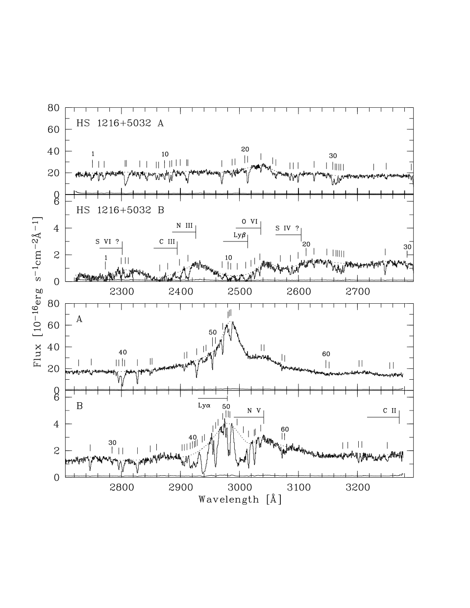
Figure 1: HST FOS G270H spectra of HS 1216+5032 A and B and their 1$\sigma$ errors. The dotted line represents the fitted continuum (§ 2.3) and the ticks mark the positions of $3\sigma$ absorption lines (§ 3), with exception of less significant C iv and Mg ii doublet lines whose identification is supported by the detection of the corresponding Ly$\alpha$ line (see § 3 and Tables 1 and 2). The vertical bars in the B plots indicate the expected position of emission lines at $z_{e}=1.451$. The horizontal bars correspond to a velocity of $5\,000$ km s^-1 in the QSO rest frame, a region thought to be affected by the BALs (see also Fig. 2). Notice in B the broad troughs on the blue side of the S iv, O vi, N iii, C iii and possibly S vi resonance lines.

Since we are interested in comparing absorption systems along both LOSs, we must check for possible small misalignments of the zero-point wavelength scale between both spectra. Such differences may arise when the targets have not been properly centered in the aperture of the FOS, and/or when – unlike here – the science and wavelength calibration exposures have not been performed consecutively. Galactic absorption lines common to both spectra were then required to appear at the same wavelength, under the assumption that both LOSs cross the same cloud (which should be true for the small separation between LOSs at $z\approx 0$). There are two Galactic absorption lines, Fe ii $\lambda 2600$ and Mg ii $\lambda 2796$, common to both spectra and apparently not contaminated with intergalactic lines. For these lines $\Delta\lambda$(Fe ii $\lambda 2600$)$=-9$ km s^-1 and $\Delta\lambda$(Mg ii $\lambda 2796$)$=+4$ km s^-1 are obtained, which lie within the fitting procedure errors ($\sim 10$ km s^-1) and the FOS limiting accuracy ($\sim 20$ km s^-1). These small differences imply that both spectra are well-calibrated; consequently, we made no corrections to the zero-point wavelength scale.

2.2 Emission redshifts

To derive the emission redshift of HS 1216+5032 A the Ly$\alpha$ emission peak was fitted with a Gaussian in the region between 2959 and 3005 Å. Excluding the wavelength regions with absorption features in the blue wing of the line yields $z_{e}({\rm A})=1.4545\pm 0.0001$, where the $1\sigma$ error comes from the wavelength uncertainty. For QSO component B, a similar analysis is extremely difficult because the Ly$\alpha$ emission line is severely distorted by the Ly$\alpha$ and N v BALs. Fitting instead the N v emission peak between 3016 and 3065 Å, and using the mean rest-frame wavelength of the doublet $\lambda_{0}$(N v)$=1240.15$ Å, yields $z_{e}({\rm B})=1.4509\pm 0.0006$. In the following we adopt the nominal values $z_{e}$(A)$=1.455$ and $z_{e}$(B)$=1.451$.

The redshifts of A and B are not the same within measurement errors, with QSO component B being blueshifted by $\sim 400$ km s^-1 relative to A. Different emission redshifts are expected in the physical pair hypothesis, but the measured difference between HS 1216+5032 A and B cannot rule out the possibility that the QSO may still be gravitationally lensed. This is because two different transitions, Ly$\alpha$ and N v, are being compared and blueshifts of a few hundreds km s^-1 between high and low-ionization emission lines are common (e.g., Hamann et al. Hamman (1997); Tytler & Fan Tytler (1992)). This point is further discussed in § 6.1.

Other prominent emission lines in the spectrum of A are: O vi $\lambda 1033$ (blended with Ly$\beta$) and probably C iii $\lambda 977$ and S iv $\lambda 1062$. In the spectrum of B, the BAL troughs allow clear identification of only Ly$\alpha$ and N v $\lambda 1240$, but the “undulating” shape of the observed flux for $\lambda<2600$ Å suggests that S vi $\lambda 939$, C iii $\lambda 977$, N iii $\lambda 990$, O vi $\lambda 1033$, and S iv $\lambda 1062$ have broad absorption troughs on the blue side of the expected QSO rest wavelengths.

2.3 Continuum fitting

Due to line blending in the Ly$\alpha$ forest, defining a quasar continuum shortward of Ly$\alpha$ emission is not trivial at our resolution. For B, this difficulty is increased by the BAL profiles. A power-law shaped continuum $f\propto\nu^{\alpha}$, although an acceptable representation in the optical range, is definitively not able to fit even the UV continuum spectrum of quasar image A, leaving residuals far larger than 3 $\sigma$ at apparently featureless spectral regions.

We decided to fit the UV QSO continuum for each spectrum with cubic splines, using the following simple and semi-automated fit algorithm. First, cubic splines are fitted through a given number of points $(x_{i},y_{i})$ thought to represent the continuum, typically 50 in each spectrum. The point ordinates $y_{i}$ are then corrected by an amount, such that the mean of the differences between the new ordinate and all the flux values within $1\sigma$ (defined by the first fit) in a 6 Å wide spectral window around $x_{i}$ equals zero. The corrected $(x_{i},y_{i})$ are used to perform a new fit. This procedure is iterated until it converges to a reasonable continuum, provided enough featureless regions are available in the data. The fit routine is robust in the sense that different start values always lead to the same continuum, but the spectral windows need to be carefully chosen, especially in the B spectrum. The final continuum is shown as dotted line in Fig. 1. Note that we have not attempted to model the QSO intrinsic continuum of B, which is evidently distorted by the BALs. Division of the flux by this continuum results in the normalized spectra of HS 1216+5032 A and B.

3 Absorption line parameters and identifications

Table 1: Absorption Lines in HS 1216+5032 A.

$$\begin{array}[]{rccccclrc}\hline\cr\vskip 3.0pt plus 1.0pt minus 1.0pt\cr{\rm Line}&\lambda_{\rm obs}&\sigma_{\lambda}&{\rm FWHM}&W_{\lambda}&\sigma_{W}&\lx@intercol\hfil\rm ID\hfil\lx@intercol&\lx@intercol\hfil z\hfil\lx@intercol&{\rm note}\\ \vskip 3.0pt plus 1.0pt minus 1.0pt\cr\hline\cr\vskip 3.0pt plus 1.0pt minus 1.0pt\cr 1&2250.88&0.44&4.99&1.27&0.27&{H\textsc{i}}\leavevmode\nobreak\ 1215&0.85155&\\ 2&2261.61&0.12&2.10&0.81&0.15&{H\textsc{i}}\leavevmode\nobreak\ 972&1.32548&\\ 3&2270.72&0.19&4.31&1.42&0.20&{H\textsc{i}}\leavevmode\nobreak\ 1215&0.86787&\\ 4&2306.20&0.16&2.22&0.58&0.19&{H\textsc{i}}\leavevmode\nobreak\ 1215&0.89706&\\ 5&2308.44&0.31&6.66&3.29&0.32&{H\textsc{i}}\leavevmode\nobreak\ 1215&0.89890&\\ 6&2331.07&0.16&2.64&0.75&0.14&{H\textsc{i}}\leavevmode\nobreak\ 1215&0.91752&\\ 7&2342.94&0.17&4.21&1.42&0.19&{Fe\textsc{ii}}\leavevmode\nobreak\ 2344&-0.00054&1\\ 8&2359.20&0.15&2.45&0.75&0.14&{H\textsc{i}}\leavevmode\nobreak\ 1215&0.94066&\\ 9&2363.08&0.14&2.41&0.79&0.15&{H\textsc{i}}\leavevmode\nobreak\ 1215&0.94385&10\\ 10&2373.10&0.14&2.46&0.77&0.13&{H\textsc{i}}\leavevmode\nobreak\ 1215&0.95210&\\ 11&2381.84&0.10&2.26&0.99&0.13&{Fe\textsc{ii}}\leavevmode\nobreak\ 2382&-0.00039&1\\ 12&2385.30&0.10&2.32&0.99&0.14&{H\textsc{i}}\leavevmode\nobreak\ 1025&1.32548&6\\ 13&2392.87&0.19&2.61&0.57&0.13&{Si\textsc{iv}}\leavevmode\nobreak\ 1393&0.71690&\\ 14&2399.75&0.45&5.76&0.84&0.23&{H\textsc{i}}\leavevmode\nobreak\ 1215&0.97402&2\\ 15&2410.50&0.28&6.18&2.28&0.23&{H\textsc{i}}\leavevmode\nobreak\ 1215&0.98285&\\ 16&2412.67&0.11&1.58&0.43&0.12&{H\textsc{i}}\leavevmode\nobreak\ 1215&0.98464&\\ 17&2470.24&0.08&3.38&1.82&0.12&{H\textsc{i}}\leavevmode\nobreak\ 1215&1.03200&3\\ 18&2487.68&0.13&1.69&0.46&0.11&{H\textsc{i}}\leavevmode\nobreak\ 1215&1.04635&\\ 19&2492.54&0.21&2.09&0.46&0.15&{H\textsc{i}}\leavevmode\nobreak\ 1025&1.43003&\\ 20&2509.24&0.28&3.39&0.55&0.15&{H\textsc{i}}\leavevmode\nobreak\ 1215&1.06408&4\\ 21&2513.90&0.14&2.66&1.60&0.25&{H\textsc{i}}\leavevmode\nobreak\ 1215&1.06791&\\ 22&2536.43&0.12&2.07&0.49&0.09&{H\textsc{i}}\leavevmode\nobreak\ 1215&1.08644&5\\ 23&2556.38&0.32&4.46&0.86&0.19&{H\textsc{i}}\leavevmode\nobreak\ 1215&1.10286&\\ 24&2561.73&0.18&3.45&1.04&0.15&{H\textsc{i}}\leavevmode\nobreak\ 1215&1.10726&7\\ 25&2585.71&0.11&2.03&0.64&0.11&{Fe\textsc{ii}}\leavevmode\nobreak\ 2586&-0.00036&1\\ 26&2591.15&0.12&2.02&0.65&0.11&{H\textsc{i}}\leavevmode\nobreak\ 1215&1.13146&\\ 27&2599.35&0.07&1.98&0.88&0.10&{Fe\textsc{ii}}\leavevmode\nobreak\ 2600&-0.00032&1\\ 28&2626.59&0.08&2.27&0.89&0.10&{H\textsc{i}}\leavevmode\nobreak\ 1215&1.16062&\\ 29&2647.53&0.17&1.74&0.34&0.10&{C\textsc{ii}}\leavevmode\nobreak\ 1334&0.98387&\\ 30&2658.10&0.12&3.17&1.77&0.18&{C\textsc{iv}}\leavevmode\nobreak\ 1548&0.71690&\\ 31&2662.31&1.00&3.01&1.20&0.83&{C\textsc{iv}}\leavevmode\nobreak\ 1550&0.71677&\\ 32&2664.83&1.00&2.88&1.11&0.81&{C\textsc{iv}}\leavevmode\nobreak\ 1548&0.72125&\\ 33&2668.68&0.11&2.02&0.84&0.15&{C\textsc{iv}}\leavevmode\nobreak\ 1550&0.72087&\\ 34&2671.66&0.20&2.47&0.62&0.15&{C\textsc{iv}}\leavevmode\nobreak\ 1548&0.72566&\\ 35&2676.23&0.23&1.92&0.28&0.11&{C\textsc{iv}}\leavevmode\nobreak\ 1550&0.72574&\\ 36&2727.61&0.16&1.80&0.35&0.10&{H\textsc{i}}\leavevmode\nobreak\ 1215&1.24371&\\ 37&2748.87&0.22&4.18&0.87&0.15&{H\textsc{i}}\leavevmode\nobreak\ 1215&1.26119&\\ 38&2791.18&0.11&1.28&0.30&0.08&{H\textsc{i}}\leavevmode\nobreak\ 1215&1.29600&\\ 39&2795.61&0.07&3.23&1.88&0.13&{Mg\textsc{ii}}\leavevmode\nobreak\ 2796&-0.00027&1\\ 40&2801.78&0.09&3.51&2.83&0.18&{Mg\textsc{ii}}\leavevmode\nobreak\ 2803&-0.00063&1\\ 41&2805.50&0.27&2.89&0.73&0.17&{H\textsc{i}}\leavevmode\nobreak\ 1215&1.30778&\\ 42&2826.96&0.04&2.43&1.77&0.09&{H\textsc{i}}\leavevmode\nobreak\ 1215&1.32543&\\ 43&2848.74&0.15&1.76&0.41&0.10&{H\textsc{i}}\leavevmode\nobreak\ 1215&1.34335&\\ 44&2851.83&0.24&2.52&0.44&0.13&{H\textsc{i}}\leavevmode\nobreak\ 1215&1.34589&\\ 45&2906.67&0.11&2.27&0.64&0.10&{H\textsc{i}}\leavevmode\nobreak\ 1215&1.39100&9\\ 46&2910.77&0.26&2.68&0.35&0.11&{H\textsc{i}}\leavevmode\nobreak\ 1215&1.39437&9\\ 47&2927.54&0.06&4.24&2.33&0.10&{H\textsc{i}}\leavevmode\nobreak\ 1215&1.40817&\\ 48&2939.28&2.20&4.83&0.64&0.52&{C\textsc{iv}}\leavevmode\nobreak\ 1548&0.89852&11\\ 49&2943.34&2.05&4.57&0.59&0.53&{C\textsc{iv}}\leavevmode\nobreak\ 1550&0.89799&11\\ 50&2954.28&0.05&2.38&1.11&0.07&{H\textsc{i}}\leavevmode\nobreak\ 1215&1.43016&\\ 51&2959.27&0.12&2.08&0.38&0.07&{H\textsc{i}}\leavevmode\nobreak\ 1215&1.43427&\\ 52&2971.79&0.06&2.83&1.04&0.07&{H\textsc{i}}\leavevmode\nobreak\ 1215&1.44457&\\ 53&2980.60&0.18&1.70&0.25&0.07&{H\textsc{i}}\leavevmode\nobreak\ 1215&1.45182&8\\ 54&2982.93&0.17&1.85&0.34&0.11&{H\textsc{i}}\leavevmode\nobreak\ 1215&1.45373&8\\ 55&2985.43&0.17&2.76&0.84&0.11&{H\textsc{i}}\leavevmode\nobreak\ 1215&1.45579&8\\ 56&3037.03&0.38&1.78&0.11&0.07&{C\textsc{iv}}\leavevmode\nobreak\ 1548&0.96166&\\ 57&3041.81&0.53&1.87&0.09&0.08&{C\textsc{iv}}\leavevmode\nobreak\ 1550&0.96148&\\ 58&3072.14&0.15&1.46&0.25&0.08&{C\textsc{iv}}\leavevmode\nobreak\ 1548&0.98434&\\ 59&3076.81&0.23&1.15&0.11&0.07&{C\textsc{iv}}\leavevmode\nobreak\ 1550&0.98405&\\ 60&3146.54&0.58&4.98&0.49&0.18&{C\textsc{iv}}\leavevmode\nobreak\ 1548&1.03239&\\ 61&3151.91&0.19&1.13&0.15&0.08&{C\textsc{iv}}\leavevmode\nobreak\ 1550&1.03248&\\ 62&3202.78&0.56&2.44&0.17&0.12&{C\textsc{iv}}\leavevmode\nobreak\ 1548&1.06872&\\ 63&3207.82&0.70&2.54&0.15&0.13&{C\textsc{iv}}\leavevmode\nobreak\ 1550&1.06853&\\ 64&3254.73&0.59&4.53&0.47&0.20&{C\textsc{iv}}\leavevmode\nobreak\ 1548&1.10227&\\ 65&3260.87&0.24&1.84&0.30&0.12&{C\textsc{iv}}\leavevmode\nobreak\ 1550&1.10275&\\ \vskip 3.0pt plus 1.0pt minus 1.0pt\cr\hline\cr\end{array}$$

• Absorption in the ISM.

• Or Si iv $\lambda 1402$ at $z=0.721$.

• Blended with H i $\lambda 1025$ at $z=1.4082$ if $b>30$ km s^-1.

• Or Si ii $\lambda 1260$ at $z=0.984$.

• Or Si iii $\lambda 1206$ at $z=1.102$.

• Blended with H i $\lambda 1215$ at $z=0.9616$.

• Or Si ii $\lambda 1260$ at $z=1.032$.

• Associated system. Ly$\beta$ is blended with line A21.

• Lines mimic C iv doublet but no corresponding H i $\lambda 1215$ line is detected.

• Small contribution from H i $\lambda 972$ at $z=1.430$ to $W_{\lambda}$.

• Strong blend. The identification is supported by the detection of H i (A4 and A5)

Table 2: Absorption Lines in HS 1216+5032 B.

$$\begin{array}[]{rccccclrc}\hline\cr\vskip 3.0pt plus 1.0pt minus 1.0pt\cr{\rm Line}&\lambda_{\rm obs}&\sigma_{\lambda}&{\rm FWHM}&W_{\lambda}&\sigma_{W}&\lx@intercol\hfil\rm ID\hfil\lx@intercol&\lx@intercol\hfil z\hfil\lx@intercol&{\rm note}\\ \vskip 3.0pt plus 1.0pt minus 1.0pt\cr\hline\cr\vskip 3.0pt plus 1.0pt minus 1.0pt\cr 1&2272.88&0.34&6.60&6.41&1.10&{S\textsc{vi}}\leavevmode\nobreak\ 933&1.43511&\\ 2&2299.56&0.19&3.44&2.57&0.44&{S\textsc{vi}}\leavevmode\nobreak\ 944&1.43463&\\ 3&2306.60&0.46&3.91&2.52&0.73&{H\textsc{i}}\leavevmode\nobreak\ 1215&0.89739&\\ 4&2311.73&0.66&5.61&3.49&1.01&{H\textsc{i}}\leavevmode\nobreak\ 1215&0.90161&\\ 5&2364.96&0.64&10.1&8.49&1.76&{C\textsc{iii}}\leavevmode\nobreak\ 977{\rm BAL}&1.42058&\\ 6&2378.32&0.25&2.72&2.62&0.81&{C\textsc{iii}}\leavevmode\nobreak\ 977{\rm BAL}&1.43426&2\\ 7&2398.41&0.32&6.99&5.26&0.74&{N\textsc{iii}}\leavevmode\nobreak\ 989{\rm BAL}&1.42313&\\ 8&2412.84&0.24&5.42&4.70&0.69&{N\textsc{iii}}\leavevmode\nobreak\ 989{\rm BAL}&1.35233&3\\ 9&2470.63&0.36&4.05&2.93&0.88&{H\textsc{i}}\leavevmode\nobreak\ 1215&1.03232&6\\ 10&2480.74&0.47&3.84&3.10&0.82&{H\textsc{i}}\leavevmode\nobreak\ 1025{\rm BAL}&1.41853&\\ 11&2485.24&0.55&4.13&3.06&0.94&{H\textsc{i}}\leavevmode\nobreak\ 1025{\rm BAL}&1.42292&\\ 12&2496.28&0.35&8.62&7.34&0.93&{O\textsc{vi}}\leavevmode\nobreak\ 1031{\rm BAL}&1.41905&\\ 13&2510.67&1.00&6.48&6.14&1.74&{O\textsc{vi}}\leavevmode\nobreak\ 1031{\rm BAL}&1.43299&4\\ 14&2519.51&0.39&4.43&2.40&0.63&{O\textsc{vi}}\leavevmode\nobreak\ 1031{\rm BAL}&1.44156&\\ 15&2525.86&0.12&2.62&1.98&0.27&{O\textsc{vi}}\leavevmode\nobreak\ 1037{\rm BAL}&1.43429&\\ 16&2534.59&0.25&1.70&1.12&0.33&{O\textsc{vi}}\leavevmode\nobreak\ 1037{\rm BAL}&1.44270&\\ 17&2569.40&0.28&2.84&0.84&0.26&{S\textsc{iv}}\leavevmode\nobreak\ 1062{\rm BAL?}&1.41789&\\ 18&2586.38&0.21&3.28&1.78&0.32&{Fe\textsc{ii}}\leavevmode\nobreak\ 2586&-0.00010&1,5\\ 19&2599.43&0.13&2.42&1.10&0.22&{Fe\textsc{ii}}\leavevmode\nobreak\ 2600&-0.00029&1\\ 20&2612.86&0.33&4.21&1.01&0.25&{H\textsc{i}}\leavevmode\nobreak\ 1215&1.14932&\\ 21&2626.39&0.21&3.18&1.01&0.20&{H\textsc{i}}\leavevmode\nobreak\ 1215&1.16045&\\ 22&2648.20&0.17&1.81&0.57&0.16&{C\textsc{ii}}\leavevmode\nobreak\ 1334&0.98437&\\ 23&2658.72&0.21&3.10&1.24&0.24&{C\textsc{iv}}\leavevmode\nobreak\ 1548&0.71730&\\ 24&2663.43&1.09&2.97&1.21&0.84&{C\textsc{iv}}\leavevmode\nobreak\ 1550&0.71749&\\ 25&2665.83&0.79&2.34&0.86&0.82&{C\textsc{iv}}\leavevmode\nobreak\ 1548&0.72190&\\ 26&2669.14&0.26&2.40&0.96&0.35&{C\textsc{iv}}\leavevmode\nobreak\ 1550&0.72117&\\ 27&2672.69&0.20&3.43&2.04&0.43&{C\textsc{iv}}\leavevmode\nobreak\ 1548&0.72633&\\ 28&2677.01&0.15&2.50&1.31&0.22&{C\textsc{iv}}\leavevmode\nobreak\ 1550&0.72625&\\ 29&2747.05&0.10&3.49&2.21&0.18&{H\textsc{i}}\leavevmode\nobreak\ 1215&1.25970&11\\ 30&2784.24&0.29&2.97&0.72&0.22&{Si\textsc{iv}}\leavevmode\nobreak\ 1402&0.98482&\\ 31&2795.57&0.10&2.42&1.39&0.18&{Mg\textsc{ii}}\leavevmode\nobreak\ 2796&-0.00028&1\\ 32&2802.26&0.55&3.68&2.57&0.69&{Mg\textsc{ii}}\leavevmode\nobreak\ 2803&-0.00045&1\\ 33&2827.11&0.10&3.39&2.69&0.27&{H\textsc{i}}\leavevmode\nobreak\ 1215&1.32556&\\ 34&2848.69&0.30&2.88&0.70&0.23&{H\textsc{i}}\leavevmode\nobreak\ 1215&1.34331&\\ 35&2859.71&0.23&2.49&0.62&0.17&{H\textsc{i}}\leavevmode\nobreak\ 1215&1.35237&\\ 36&2902.79&0.47&3.39&1.04&0.33&{H\textsc{i}}\leavevmode\nobreak\ 1215&1.38781&\\ 37&2906.60&0.30&3.20&1.45&0.32&{H\textsc{i}}\leavevmode\nobreak\ 1215&1.39094&7\\ 38&2911.22&0.16&1.91&0.59&0.15&{H\textsc{i}}\leavevmode\nobreak\ 1215&1.39475&7\\ 39&2916.57&0.33&2.94&1.49&0.54&{Mg\textsc{ii}}\leavevmode\nobreak\ 2796&0.04299&8\\ 40&2920.25&0.47&4.67&2.64&0.92&{Mg\textsc{ii}}\leavevmode\nobreak\ 2796&0.04431&8\\ 41&2923.58&0.19&1.22&0.31&0.23&{Mg\textsc{ii}}\leavevmode\nobreak\ 2803&0.04282&8\\ 42&2925.69&0.48&2.94&1.64&0.94&{Mg\textsc{ii}}\leavevmode\nobreak\ 2803&0.04357&8\\ 43&2928.69&1.13&3.53&1.42&0.77&{H\textsc{i}}\leavevmode\nobreak\ 1215?&1.40912&\\ 44&2936.95&0.14&3.29&1.06&0.24&{H\textsc{i}}\leavevmode\nobreak\ 1215{\rm BAL}&1.41591&\\ 45&2940.68&0.24&9.41&8.06&0.37&{H\textsc{i}}\leavevmode\nobreak\ 1215{\rm BAL}&1.41898&\\ 46&2954.99&0.07&1.33&0.56&0.09&{H\textsc{i}}\leavevmode\nobreak\ 1215&1.43075&\\ 47&2959.60&0.06&4.41&3.61&0.18&{H\textsc{i}}\leavevmode\nobreak\ 1215{\rm BAL}&1.43454&\\ 48&2963.76&0.18&2.18&0.48&0.12&{H\textsc{i}}\leavevmode\nobreak\ 1215{\rm BAL}&1.43796&\\ 49&2971.75&0.26&3.33&0.52&0.13&{H\textsc{i}}\leavevmode\nobreak\ 1215&1.44454&\\ 50&2977.11&0.09&1.50&0.45&0.08&{H\textsc{i}}\leavevmode\nobreak\ 1215&1.44895&\\ 51&2981.12&0.12&2.66&1.66&0.17&{H\textsc{i}}\leavevmode\nobreak\ 1215&1.45224&9\\ 52&2983.79&0.11&2.23&1.28&0.14&{H\textsc{i}}\leavevmode\nobreak\ 1215&1.45444&9\\ 53&2996.12&0.29&9.16&6.52&0.46&{N\textsc{v}}\leavevmode\nobreak\ 1238{\rm BAL}&1.41853&\\ 54&3006.67&0.41&11.4&6.81&0.69&{N\textsc{v}}\leavevmode\nobreak\ 1242{\rm BAL}&1.41926&\\ 55&3015.40&0.06&3.94&2.86&0.14&{N\textsc{v}}\leavevmode\nobreak\ 1238&1.43409&\\ 56&3025.12&1.00&2.58&1.52&0.67&{N\textsc{v}}\leavevmode\nobreak\ 1242&1.43411&\\ 57&3026.94&1.86&2.43&0.66&1.25&{N\textsc{v}}\leavevmode\nobreak\ 1238&1.44340&\\ 58&3036.12&0.46&1.47&0.34&0.31&{N\textsc{v}}\leavevmode\nobreak\ 1242&1.44296&\\ 59&3072.15&0.15&1.76&0.53&0.17&{C\textsc{iv}}\leavevmode\nobreak\ 1548&0.98434&\\ 60&3076.58&0.54&6.86&1.50&0.43&{C\textsc{iv}}\leavevmode\nobreak\ 1550&0.98390&\\ 61&3175.03&0.40&2.98&0.45&0.19&{Mg\textsc{ii}}\leavevmode\nobreak\ 2796&0.13542&\\ 62&3183.64&0.55&2.91&0.35&0.23&{Mg\textsc{ii}}\leavevmode\nobreak\ 2803&0.13558&\\ 63&3201.81&0.15&3.13&1.21&0.18&{C\textsc{iv}}\leavevmode\nobreak\ 1548&1.06809&\\ 64&3207.46&0.20&3.36&1.06&0.20&{C\textsc{iv}}\leavevmode\nobreak\ 1550&1.06830&\\ 65&3250.52&0.58&5.02&1.53&0.41&{C\textsc{ii}}\leavevmode\nobreak\ 1334{\rm BAL}&1.43570&10\\ \vskip 3.0pt plus 1.0pt minus 1.0pt\cr\hline\cr\end{array}$$

• Absorption in the ISM.

• Probably blended with Ly-$\alpha$.

• Blended with Ly$\alpha$ at $z=0.984$.

• Blended with H i $\lambda 1025$ BAL.

• Also S iv $\lambda 1062$ BAL because the line is too strong compared with IS Fe ii $\lambda 2600$.

• Or H i $\lambda 1025$ at $z=1.4082$ if $b>30$ km s^-1.

• Lines mimic C iv doublet but no corresponding H i $\lambda 1215$ line is detected.

• The fit procedure is not able to resolve the second doublet lines; therefore, the doublet ratios are probably not real.

• Associated system. Ly$\beta$ falls in the O vi BAL troughs.

• Blended with C ii${}^{*}\leavevmode\nobreak\ \lambda 1035$. See § 5 for the classification as BAL system.

• No line at $3\sigma$ can be identified with Ly$\beta$.

Tables 1 and 2 list absorption lines found at the $3\sigma$ level in HS 1216+5032 A and B, respectively. Lines in the normalized spectra were fitted with Gaussian profiles without constraints in central wavelength, width or amplitude. In the case of obvious blends two or more Gaussian components were fitted simultaneously.

The fit routine attempts to minimize $\chi^{2}$ between model and data, considering $1\sigma$ flux errors (flat-fielding, background subtraction and photon statistics noise); but the uncertainties introduced by the continuum placement are not included.

An inherent feature of $\chi^{2}$ minimization is the non-uniqueness of the solution due to the eventual presence of more than one minimum in the parameter space. In those cases, the fit can lead not only to wrong parameter estimations but also to underestimated parameter errors. To handle with this problem, instead of defining a rejection parameter we simply performed several fit trials taking different wavelength ranges to see how robust a particular solution was. In general, there were no significant changes in the resulting parameters due to a different choice of the fitting interval, thus giving us confidence on the results. However, some fits yield $\chi^{2}_{\nu}<1$. Assuming that the $1\sigma$ flux errors are not overestimated, such behaviour can occur by chance, especially when too few pixels are considered in the fit.

The equivalent-width error estimates are generally larger than the propagated error if the flux values are integrated along a line. This is because the former errors consider the correlation between all three free parameters. This is not the case for multicomponent fits, where the errors in equivalent width may be overestimated since the fit algorithm does not consider that the strengths and widths of neighbour lines in blends are anti-correlated.

Concerning the line widths, note that several FWHM values in Tables 1 and 2 are slightly larger than the nominal width of the line spread function (LSF), $2$ Å. This is caused by the difficulty in resolving absorption structures separated by less than $\sim 200$ km s^-1, since single-line fits of closely lying line complexes (blends) will inevitably lead to large widths. On the other hand, in few cases the measured lines are narrower than the LSF. While this might partly be caused by a too low placement of the continuum near emission lines and BAL troughs in the B spectrum, it is certainly not the case for all the narrow lines in the A spectrum. In the latter case fitting weak lines also leads to low FWHM values (with large associated errors), thus reflecting the limitations of the $\chi^{2}$ minimization using too few pixels.

BAL profiles in the B spectrum have been fitted with multicomponent Gaussians to better constrain their equivalent widths, but these fits do not necessarily represent the actual nature of the BAL profiles (see § 5). For consistency, Tables 1 and 2 include the Gaussian parameters of BAL profiles.

Absorption lines were identified manually, using vacuum wavelengths and oscillator strengths taken from Verner et al. (Verner (1994)). The identification of lines is not easy because of the low resolution and the lack of optical data; but it is especially difficult in the B spectrum because narrow intergalactic lines are hidden among the BALs. We looked first for interstellar absorption lines in both spectra. The Mg ii $\lambda 2796,2803$ doublet and the Fe ii lines at 2586 Å and 2600 Å are detected in both spectra; the Fe ii lines at 2344 Å and 2382 Å are detected at $3\sigma$ only in the A spectrum (while in the B spectrum Fe ii $\lambda 2382$ would appear at the position of BAL C iii $\lambda 977$). The next step was to search for C iv systems and their associated Ly$\alpha$ and prominent metal lines. In addition, two Mg ii systems at $z=0.04$ (§ 4.2) and $1.14$ could be identified in the spectrum of B through the positions of the doublet lines and their relative strengths. Due to their secure identification, C iv $\lambda 1548,1550$ and Mg ii $\lambda 2796,2803$ lines with ${\rm SNR}<3$ have been retained in Tables 1 and 2, which otherwise contain only lines with ${\rm SNR}>3$. Ly$\alpha$ lines with redshifts of $1.16<z<z_{e}$ were identified through the corresponding Ly$\beta$ and Ly$\gamma$ lines, if present. Lines A45, A46, B37, and B38 mimic a C iv doublet at $z=0.88$, but since no significant absorption by H i is detected at this redshift, they have been counted as Ly$\alpha$ lines. The remaining lines have been considered to be Ly$\alpha$ lines and will be discussed in § 6.

4 Metal absorption systems in HS 1216+5032 A and B

We now give a description of the most remarkable metal absorption systems observed in HS 1216+5032 A and B: a Mg ii system at $z=0.04$, and a strong C iv system at $z=0.72$.

4.1 The C iv systems at $\mathit{z=0.72}$ in HS 1216+5032 A and B

Three strong C iv systems at $z=0.717$, $0.721$ and $0.726$ are identified through the $\lambda\lambda 1548,1550$ doublets at $\lambda\sim 2660$ Å in both spectra of HS 1216+5032. Although some of the C iv lines are under the $3\sigma$ significance level, the well-determined redshifts of the doublet components make their identification unambiguous; consequently, all six C iv lines appear in Tables 1 and 2.

The rest frame equivalent widths of the $\lambda 1548$ lines range between $0.36$ and $1.03$ Å in the A spectrum, and between 0.72 and 1.19 Å in B. The large column densities implied by these line strengths, make this system a firm candidate for a Lyman-limit system (Sargent, Steidel & Boksenberg Sargent (1989)). Also, the large line widths in A and B, FWHM $>2$ Å, suggest that these C iv systems will reveal several narrower components at higher resolution.

No further metal lines are found at these redshifts. Line A13 could be identified with Si iv $\lambda 1393$ at $z=0.717$, but two strong Ly$\alpha$ lines at $\lambda=2410$ Å make the detection of the second doublet line impossible. No transitions by low-ionization species (e. g., C ii $\lambda 1334$) are detected. In the low-resolution optical spectrum of HS 1216+5032 B (see Fig. [3] in Hagen et al. Hagen (1996)), a significant absorption feature at $\lambda=4816$ Å could tentatively be identified with a Mg ii $\lambda 2796,2803$ doublet associated to these C iv systems, but no absorption feature is seen at this wavelength in the optical spectrum of A.

The small velocity differences of $\Delta v_{\rm A-B}\approx-68\pm 28$ km s^-1, $-52\pm 31$ km s^-1, and $-116\pm 30$ km s^-1 at $z=0.717$, $0.721$ and $0.726$, respectively, between the C iv lines in A and the corresponding ones in B suggest strongly that these C iv systems are physically associated. Therefore, the large velocity span of roughly $1500$ km s^-1 along each LOS can only be explained if the gas is virialized by a cluster of galaxies. The virial mass within the radius given by the half separation between the LOSs is derived to be $\sim 10^{13}$ M_⊙. Consequently, if C iv systems arise in the extended halos of galaxies (Bergeron & Boisse Bergeron (1991)), the present data gives evidence that the C iv absorbers at $z=0.72$ in HS 1216+5032 A and B arise either in the highly ionized intra-group gas of a galaxy cluster, or in small structures associated with the cluster.

The whole absorption complex shows an asymmetry in the sense that the weakest system in spectrum A has the same redshift as the strongest in B: the ratio of the $\lambda 1548$ line’s equivalent width in A to that in B varies between 1.4 and 3.3. If C iv systems in A and B with similar redshifts are physically associated, then the different line strengths have direct implications for the size of these absorbers. This is because such gas inhomogeneities imply that the LOSs sample the clouds on spatial scales similar to the transverse cloud sizes. The interpretation remains valid if the lines in the present FOS spectra result from many unresolved velocity components, because in that case stronger lines result from more narrow components than weaker lines do, a picture that is still compatible with gas inhomogeneities. All these three C iv absorption systems should therefore arise in clouds with characteristic transverse lengths of $\sim 75\leavevmode\nobreak\ h_{50}^{-1}$kpc, larger than the statistical lower limits of $\sim 30\leavevmode\nobreak\ h_{50}^{-1}$kpc derived by Smette et al. (Smette (1995)) for C iv absorbers at $z\ga 1.5$.

Alternatively, it is still possible that the C iv absorption is correlated in redshift, but occurs in distinct, separated structures. At higher resolution, Rauch (Rauch1 (1997)) has shown that in gas associated with metal systems density gradients on sub-kpc scales are not uncommon. The logical conclusion would be that C iv absorbers are composed of a large number of small cloudlets. However, if that is the case of the $z=0.72$ absorbers, the correlation in redshift between lines in A and B is difficult to explain without invoking cloudlets aligned along a filamentary or sheet-like structure.

4.2 A Mg ii System at $\mathit{z=0.04}$ in HS 1216+5032 B?

There is a strong and blended feature at $\lambda\sim 2920$ Å in the B spectrum for which we do not find any plausible identification with other observed metal systems. One possible identification is absorption by two Mg ii $\lambda\lambda 2796,2803$ doublets at $z=0.043$ and $z=0.044$. Although the Gaussian profile fit is not able to resolve the single lines in the red trough of the absorption feature, the identification is supported by a good match between the line positions and profiles of the doublet. The red wing of the whole absorption feature could be blended with a Ly$\alpha$ line because it coincides quite well with a strong Ly$\alpha$ line at $z=1.4$ in A (A47). However, no Fe ii lines are detected at this redshift, nor further transitions by low-ionization species. The Mg i $\lambda 2852$ line is possibly present, but the match in wavelength with line B50, $\Delta\lambda\approx 1.4$ Å, is not very good. Under the Mg ii-hypothesis, the total rest-frame equivalent width of the stronger Mg ii doublet component would be $W_{0}=3.97$ Å, which is somewhat larger than typical values found in gas associated with damped Ly$\alpha$ (DLA) systems at high redshift (Lu et al. Lu (1996)) or in the Milky Way (Savage et al. Savage (1993)). This could be explained if the lines are indeed made up of several narrower components, as usually seen in DLA systems. The redshift difference between both Mg ii systems implies a velocity span of roughly 300 km s^-1, also typical of DLA systems. Therefore, there is some evidence that these Mg ii lines might be associated with a DLA system at $z=0.04$.

Regardless of the DLA-system interpretation, however, even the absence of Fe ii and – possibly – also Mg i lines associated with Mg ii of such a strength is difficult to explain considering the incidence of the former ions in Mg ii-selected samples (e.g., Bergeron & Stasinska Bergeron2 (1986); Steidel & Sargent Steidel (1992)). Consequently, an alternative identification of the $\lambda\sim 2920$ Å feature as H i $\lambda 1215$ BAL at $v\sim-6\,000$ km s^-1 (see §5 and Figure 2) must be considered as well. The absence of a corresponding H i $\lambda 1025$ BAL profile, however, is also in this case remarkable, but could be explained if the absorber does not completely cover the continuum source (see below).

5 The BAL systems in HS 1216+5032 B: Some Qualitative Inferences

Three BAL systems are observed in the UV spectrum of HS 1216+5032 B (see Fig. 2, where the system redshifts have been arbitrarily numbered 1, 2, and 3). Absorption by H i, C iii, N iii, and possibly S iv is observed in at least two of the systems, while O vi and N v are present in all three systems. C ii is observed only in system 2, and N iii in systems 2 and 3.

Many features distinguish these systems from the most commonly observed BAL systems (e.g., Turnshek et al. Turnshek (1996)): (1) the lines are particularly weak and several line profiles are not distorted by/or blended with other BALs; (2) the maximum outflow velocity $v\sim 5\,000$ km s^-1 is small compared with typical BALQSOs, which exhibit terminal velocities of several $10^{4}$ km s^-1(Turnshek Turnshek1 (1984)); (3) C ii is present (see Wampler et al. Wampler (1995) for other BAL QSO spectrum with singly-ionized species; Arav et al. 1999b ); (4) the strength of H i in systems 2 and 3 decreases more slowly at the red edge of the troughs (Turnshek Turnshek1 (1984)).

Also remarkable is the undulating shape of the absorbed continuum for $\lambda<2700$ Å (see Fig. 1). The position of the flux depressions coincides quite well with the blue wing of expected emission lines by C iii, N iii, Ly$\beta$, and O vi. This coincidence seems to suggest that the absorption is indeed dominated by very broad line components, which determine the continuum shape, superimposed to the narrower components, here labeled as systems 1, 2 and 3. The same effect, although less remarkable, is observed for S iv and S vi, thus giving evidence for absorption by these ions associated with the BAL phenomenon (also reported for another QSO by Arav et al. 1999a ).

It is customary to define BALs as a continuous absorption with outflow velocities larger than $\sim 3\,000$ km s^-1 from the emission redshift (Weymann et al. Weymann2 (1991)) to make a distinction between BAL systems and “associated systems”. However, as pointed out by Arav et al. (1999b ), such definition does not hold any physical meaning. In our case, systems 1 and 2 should be then classified as associated systems but, due to our poor resolution, it is not possible to establish whether the line profiles are produced by continuous absorption or whether they are made of several narrower velocity components (as observed in associated systems). The metal lines in these systems (e.g. the N v and O vi doublet lines) are relatively narrow and their widths could be dominated by the instrumental profile (for H i in system 2, however, the situation is less clear). Therefore, the classification of systems 1 and 2 as BAL systems must be considered solely instrumental.

High-resolution spectra of BAL QSOs (Hamann et al. Hamman (1997)) show that BAL profiles do not necessarily result from an ensemble of discrete narrow, unresolved lines, but as part of a mixture of a continuously accelerated outflow and overlapping narrow components with different non-thermal velocity dispersions. For the systems in HS 1216+5032, it can be assumed that a similar mixture of line widths is present, with the broad components dominating over the narrow ones. In that case, these line profiles should not look so different at higher resolution (with exception, maybe, of systems 1 and 2).

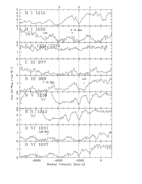
Figure 2: Broad absorption lines in HS 1216+5032 B plotted in velocity relative to $z_{e}=1.451$.

Ionization models have shown that BAL clouds span a range of densities and/or distances from the ionizing source (Turnshek et al. Turnshek (1996); Hamann et al. Hamman1 (1995)). Fig. 2 shows that, while the high-ionization species N v and O vi are present in all three systems in HS 1216+5032, H i, C ii and doubly-ionized species are absent in system 1. A possible explanation is that the ionization conditions could change with outflow velocity, with higher ionization level for redshifts closer to $z_{e}$. However, a quantitative study of the ionization conditions in these BAL clouds with the present data is made difficult by our inability to reliably establish the continuum level at the BAL troughs and thus determine column densities (besides the fact that nonblack saturation of the line profiles might be present; see Arav et al. 1999a ).

Nevertheless, a more quantitative study of the BAL phenomenon in HS 1216+5032 B should be possible using higher resolution HST spectra to better estimate the QSO continuum and to identify spurious lines at the BAL troughs. In particular, BAL system 2 can be studied in more detail because it shows more ions and less contamination by narrow absorption lines at the lines lying in the Ly$\alpha$ forest. On the other hand, alone medium-resolution optical spectra should considerably improve our knowledge of the BAL systems in HS 1216+5032 through the line profiles of C iv, C iii, and possibly Mg ii, which we suspect to be present given the presence of C ii. The width of the trough in system 2 is sufficiently small to study nonblack saturation effects via doublet ratios provided the emission line profiles can be determined (e.g., at the position of the C iv BAL). Thus, corrected column densities for system 2 appear as very suitable to reliably examine photoionization models because the radiation fields can be constrained by the presence of low-ionization species.

6 Ly$\alpha$ absorption systems

We now describe the Ly$\alpha$ forest lines observed in the spectra of HS 1216+5032 A and B. The projected separation between LOSs samples well the expected cloud sizes of hundreds of kpc if the QSO pair is real (see next subsection). However, the effective redshift path where Ly$\alpha$ lines can in principle be detected is blocked out by the broad absorption lines in the B spectrum, so the line samples will be small.

6.1 Lensed or Physical Pair?

The nature of the double images in HS 1216+5032 is not clearly established yet. Maybe the strongest arguments favoring HS 1216+5032 AB as a physical-pair instead of a gravitational lens origin are: (1) BALs are observed only in the spectrum of the B image; (2) no extended, luminous object is detected between (or even close to) the QSO images down to $m_{R}=22.5$; and (3) gravitationally lensed QSO pairs normally have image separations $\theta\la 3\arcsec$ (e.g., Kochanek, Falco & Muñoz Kochanek (1999)). In addition, the absence of a trend for equivalent widths of intervening Ly$\alpha$ lines common to both spectra to become similar at redshifts closer to $z_{e}$ (see Fig. 4 and Table 3) also argues for a physical-pair; however, this argument is weak as the sample of common lines is too small. Unfortunately, for reasons given in § 2.2, it is not possible to establish whether there are differences between A and B in the emission line redshifts and line shapes in the spectral region covered by the FOS.

The intriguing point here is that two $z\approx z_{e}$ Ly$\alpha$ systems are detected in both spectra at almost identical redshifts to within $\sim 90$ km s^-1 (see § 6.6 for more details). Under the physical-pair hypothesis, these absorbers should extend over transverse scales greater than $80\leavevmode\nobreak\ h_{50}^{-1}$kpc. If, on the other hand, HS 1216+5032 AB is a gravitationally lensed pair, the detection of these systems in both spectra can easily be explained by the fact that the separation between light paths approaches zero.

In consequence, the gravitational lens nature of HS 1216+5032 cannot be yet ruled out. Let us note that in a simple lens geometry the virial mass implied by the velocity span of the C iv absorbers at $z=0.72$ (see § 4.1) is consistent with the deflector mass required to produce an angular separation between QSO images of $\theta=9\arcsec$. In such a model the separation between light paths at the source position is derived to be $\theta_{s}=17$″. Therefore, confirmation of HS 1216+5032 as a gravitationally lensed QSO would have dramatic consequences for our understanding of the BAL phenomenon. As pointed out by Hagen et al. (Hagen (1996)), if HS 1216+5032 AB were indeed the mirror images of one unique QSO, the coverage fraction of BAL clouds would have to be very small. Incomplete coverage of the continuum source or the BLR in BAL clouds have been confirmed using high-resolution spectra (Hamann et al. Hamman (1997); Barlow & Sargent Barlow (1997)). In fact, the cloud sizes derived from BAL variability could be $10^{4}$ times smaller than the distances to the source derived from photoionization models (Hamann et al. Hamman1 (1995)), implying subtended angles not much larger than $\theta_{s}$. Therefore, the scenario in which only one light path crosses the BAL clouds is not unrealistic, and the non-BAL spectrum of HS 1216+5032 A can also be considered if the QSO pair is lensed.

In summary, there are reasons to believe that HS 1216+5032 is a binary QSO, but a gravitational lens origin of the double images cannot yet be excluded. A definitive assessment of this issue must await medium resolution optical spectra to better derive emission redshifts and to establish differences in the continuum or emission lines. Alternatively, deep infrared or radio observations would help determining the nature of the double QSO images. The non-detection of the lensing galaxy/cluster would be a strong proof for the binary QSO hypothesis, since wide separation ($\theta>3\arcsec$) “dark lenses” enter in conflict with current models of structure formation (Kochanek, Falco & Muñoz Kochanek (1999)), which predict few wide separation gravitational lenses (e.g., Kochanek Kochanek1 (1995)).

Throughout this section we will assume that HS 1216+5032 AB is a physical pair. The proper separation $S(z)$ between LOSs obeys then the relation $S=\theta\leavevmode\nobreak\ D_{\rm oc}$, where $\theta$ is the angular separation between the A and B QSO images, and $D_{\rm oc}$ is the angular-diameter distance between the observer and a cloud at redshift $z$. For the redshift range of interest $S\simeq 80$ $\leavevmode\nobreak\ h_{50}^{-1}$ kpc.

6.2 Line List

Figure 3: Three $\sigma$ rest-frame detection limits of Ly$\alpha$ lines in HS 1216+5032A (thick line) and B.

Table 3 lists Ly$\alpha$ lines detected at the $3\sigma$ level in HS 1216+5032 A and B. Figure 3 shows $3\sigma$ detection thresholds as a function of redshift. Out of 36 lines in the spectrum of A, a total of 23 lines within $z=0.85$ to $1.43$ have $W_{\rm 0}({\rm A})\geq 0.24$ Å. This redshift interval excludes lines within $3\,000$ km s^-1 from the QSO redshift to avoid the “proximity effect” (Bechtold Bechtold (1994)). The derived number density is $\log(dN/dz)=1.58^{+0.09}_{-0.10}$ at $\log(1+z)=0.33\pm 0.06$, in very good agreement with the results of the HST Key Project (Weymann et al. Weymann1 (1998)). The scarce sample of lines in B is clearly explained by the shorter redshift path allowed by the BAL profiles.

Table 3: Ly$\alpha$ Lines with $W>3\sigma_{W}$ in HS 1216+5032 A and B.

$$\begin{array}[]{crcccrcccrr}\hline\cr\vskip 3.0pt plus 1.0pt minus 1.0pt\cr\lx@intercol\hfil\rm A\hfil\lx@intercol&\lx@intercol\hfil\rm B\hfil\lx@intercol&&\lx@intercol\hfil\rm A-B\hfil\lx@intercol\\ \vskip 3.0pt plus 1.0pt minus 1.0pt\cr{\rm Line}&\lx@intercol\hfil W_{0}({\rm\AA})\hfil\lx@intercol&{\rm SNR}&z&{\rm Line}&\lx@intercol\hfil W_{0}({\rm\AA})\hfil\lx@intercol&{\rm SNR}&z&{\rm Remarks}&\lx@intercol\hfil\Delta v({\rm km\leavevmode\nobreak\ s}^{-1})\hfil\lx@intercol&\lx@intercol\hfil\Delta W_{0}\leavevmode\nobreak\ ({\rm\AA})\hfil\lx@intercol\\ \vskip 3.0pt plus 1.0pt minus 1.0pt\cr\hline\cr\vskip 3.0pt plus 1.0pt minus 1.0pt\cr 1&0.68&4.8&0.85155&&&&&1&&\\ 3&0.76&7.0&0.86787&&&&&2&&\\ 4&0.31&3.1&0.89706&3&1.33&3.5&0.89739&3&-52\pm 63&-1.02\pm 0.40\\ 5&1.73&10.2&0.89890&&<0.47&&&3&&\\ &<0.19&&&4&1.84&3.5&0.90161&4&&\\ 6&0.39&5.3&0.91752&&&&&1&&\\ 8&0.39&5.2&0.94066&&&&&1&&\\ 9&0.41&5.5&0.94385&&&&&2&&\\ 10&0.39&5.7&0.95210&&&&&1&&\\ 14&0.42&3.7&0.97402&&&&&2&&\\ 15&1.15&10.1&0.98285&&&&&2&&\\ 16&0.22&3.7&0.98464&&&&&2,3&&\\ 17&0.89&14.9&1.03200&9&1.44&3.3&1.03232&3&-47\pm 45&-0.55\pm 0.44\\ 18&0.23&4.3&1.04635&&&&&2&&\\ 20&0.27&3.7&1.06408&&&&&2&&\\ 21&0.78&6.3&1.06791&&&&&2,3&&\\ 22&0.23&5.5&1.08644&&&&&1&&\\ 23&0.41&4.7&1.10286&&&&&1,3&&\\ 24&0.49&6.9&1.10726&&&&&1&&\\ 26&0.30&5.8&1.13146&&&&&5&&\\ &<0.14&&&20&0.47&4.0&1.14932&&&\\ 28&0.41&9.1&1.16062&21&0.47&5.0&1.16045&&23\pm 26&-0.06\pm 0.10\\ 36&0.16&3.6&1.24371&&&&&5&&\\ &<0.11&&&29&0.98&12.3&1.25970&&&\\ 37&0.39&5.8&1.26119&&<0.19&&&&&\\ 38&0.13&3.8&1.29600&&&&&1&&\\ 41&0.32&4.4&1.30778&&&&&1&&\\ 42&0.76&20.0&1.32543&33&1.16&10.0&1.32556&&-16\pm 11&-0.39\pm 0.12\\ 43&0.18&4.0&1.34335&34&0.30&3.0&1.34331&&5\pm 35&-0.12\pm 0.11\\ 44&0.19&3.3&1.34589&&&&&5&&\\ &<0.10&&&35&0.26&3.6&1.35237&&&\\ &<0.10&&&36&0.44&3.2&1.38781&&&\\ 45&0.27&6.6&1.39100&37&0.61&4.5&1.39094&&7\pm 33&-0.34\pm 0.14\\ 46&0.14&3.1&1.39437&38&0.25&3.9&1.39475&&-47\pm 32&-0.10\pm 0.08\\ 47&0.97&23.2&1.40817&&&&&1&&\\ 50&0.46&15.9&1.43016&46&0.23&6.2&1.43075&&-72\pm 9&0.23\pm 0.05\\ 51&0.16&5.5&1.43427&&&&&2&&\\ 52&0.43&15.7&1.44457&49&0.21&4.0&1.44454&&4\pm 27&0.21\pm 0.06\\ &<0.11&&&50&0.18&5.6&1.44895&&&\\ 53&0.10&3.7&1.45182&51&0.68&9.8&1.45224&6&-51\pm 22&-0.58\pm 0.03\\ 54&0.14&3.1&1.45373&52&0.52&9.1&1.45444&6&-87\pm 20&-0.38\pm 0.07\\ 55&0.34&7.5&1.45579&&&&&6&&\\ \vskip 3.0pt plus 1.0pt minus 1.0pt\cr\hline\cr\end{array}$$

• Three sigma detection limits in B $>W$(A).

• Spectral region covered by the BAL troughs in B.

• C iv associated.

• Maybe S iv $\lambda$944 BAL.

• Absorption feature present in B at low significance.

• Associated system.

6.3 Definition of Line Samples

To define the number of coincidences and anti-coincidences we have selected from all 36 Ly$\alpha$ lines observed in A (the spectrum with better signal-to-noise) those ones (1) at $z\leq 1.43$; (2) not associated with metal lines; (3) at wavelengths not covered by the BAL troughs in B; and (4) at wavelengths where $3\sigma$ detection limits in B are lower than the measured equivalent width of the line in A. Lines in B that had ${\rm SNR}>3$ and fulfilled criteria (1) to (3) were also selected. In some cases, lines in A have a corresponding absorption feature at the same wavelength in B, but at a too low significance level to unambiguously designate the line pair as a coincidence. These lines in A were excluded (A26, A36, A44). Notice that criterion (3) automatically prevents comparing line equivalent widths for which the uncertainties introduced by the placement of the B continuum are large.

The final sample of Ly$\alpha$ lines suitable for this study is composed of $N=11$ redshift systems within $1.16<z<1.43$, a range not much smaller than the one allowed by conditions (1) to (4). Out of this number, $N_{\rm C}=6$ systems show Ly$\alpha$ lines in both spectra, and $N_{\rm A}=5$ lines are detected in only one spectrum. The rest-frame equivalent widths range from 0.14 to 0.76 Å in A, and from 0.23 to 1.16 Å in B. This sample is hereafter called “full sample”.

Coincident lines are shown in Figure 4, where the thick line represents the flux of A and the zero velocity point corresponds to the redshift of the A line. Only the first six panels show lines in the “full sample”; the remaining lines arise in Ly$\alpha$ clouds likely to be influenced by the QSO flux. All coincident lines are separated by less than 100 km s^-1. Anti-coincident lines are all uniquely defined, as there are no corresponding lines in the other spectrum within several hundred km s^-1.

However, there are two exceptions that must be pointed out. The first one is line 29 in B, separated by $198$ km s^-1 from the nearest Ly$\alpha$ line in A (37). These lines in A and B have been counted as anti-coincidences, though we are suspicious of this interpretation as the line profiles suggest line B29 is blended with an absorption feature seen in both spectra. The second is another of the anti-coincidences, line B50, which could alternatively be identified with Mg i at $z=0.04$. These cases will introduce unavoidable uncertainties in the results presented here. Let us recall that the exclusion of any one line from the samples would lead to significantly different results for $R_{\rm c}$. This illustrates the real uncertainties dominating simulations with such a small number of observed lines. Moreover, the samples are limited by the large redshift path blocked out by the BAL troughs in B, so there must be a considerable loss of information.

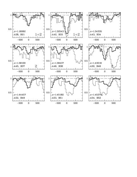
Figure 4: Ly$\alpha$ lines present both in HS 1216+5032 A and B, with ${\rm SNR}>3$, $\Delta v({\rm A-B})<100$ km s^-1, and no metals associated. These lines lie at wavelengths not covered by the BAL troughs in B. The right number indicates to which sample the line pair belongs. The three bottom panels show lines that fall within $3\,000$ km s^-1 from the QSO redshift. The thick line represents the flux of A. The abscissa is in km s^-1 and the zero-velocity point is defined by the redshift of each A line.

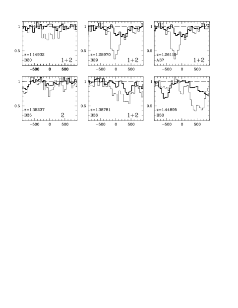
Figure 5: Ly$\alpha$ lines present either in HS 1216+5032 A or B, with ${\rm SNR}>3$, $\Delta v({\rm A-B})<100$ km s^-1, and no metals associated. These lines lie at wavelengths not covered by the BAL troughs in B. The right number indicates to which sample the line pair belongs. The abscissa is in km s^-1 and the zero-velocity point is defined by the redshift of each present line.

A line significance level of $5$ for lines in A has been chosen to perform the likelihood analysis described in the next subsection . This selection automatically excludes two of the redshift systems in the full sample and defines the following sub-samples:

1. Strong-line sample (sample 1): lines for which SNR(A) $>5$, SNR(B) $>3$, and $W_{0}>0.32$ Å. This selection yields $N_{\rm C}=2$ coincidences and $N_{\rm A}=4$ anti-coincidences.

2. Strong+weak line sample (sample 2): same as previous sample but with $W_{0}>0.17$ Å. This selection yields $N_{\rm C}=4$ and $N_{\rm A}=5$.

6.4 Maximum Likelihood Analysis

In the following we discuss a likelihood analysis on cloud sizes in front of HS 1216+5032. The technique is based on the definition of a likelihood function $\cal{L}$ that gives the probability of getting the observed number of coincidences and anti-coincidences. Evidently, such a function must depend on the shape of the absorber. Here we concentrate on two possible cloud geometries for which $\cal{L}$ can be derived analytically: spheres and cylinders.

For coherent spherical clouds, the probability that one cloud at redshift $z$ is intersected by one LOS is given by McGill (McGill (1990)) as:

$$\phi(X)=\frac{2}{\pi}\left\{\arccos\left[X(z)\right]-X(z)\sqrt{1-X(z)^{2}}\right\}\leavevmode\nobreak\ ,$$ (1)

where $X(z)\equiv S(z)/2R_{\rm c}$ and $R_{\rm c}$ is the cloud radius. The samples consider only redshifts where at least one LOS intersects a cloud (otherwise one should make assumptions on the cloud distribution along the LOS). Therefore, one must compute the probability that, given that a line appears in one spectrum, a line will appear in the other spectrum. This probability is given by Dinshaw et al. (Dinshaw2 (1997)) as:

$$\psi(X)=\frac{\phi}{2-\phi}\leavevmode\nobreak\ .$$ (2)

Finally, the probability of getting the observed number of coincidences and anti-coincidences is given by the product

$${\cal L}(R_{\rm c})=\prod_{i}\psi\left[X(z_{i})\right]\leavevmode\nobreak\ \prod_{j}\left\{1-\psi\left[X(z_{j})\right]\right\}\leavevmode\nobreak\ ,$$ (3)

where the indexes $i$ and $j$ number the coincidences and anti-coincidences, respectively. Note that if there is at least one anti-coincidence, then $\cal L$ has a maximum value. Otherwise it grows monotonically.

The solid curve in Fig. 6 shows the results of the likelihood function ${\cal L}(R_{c})$ normalized to its peak intensity for the various samples. The figure also shows the cumulative distribution of ${\cal L}(R_{c})$. The estimated $2\sigma$ limits on cloud diameters for HS 1216+5032 – derived from the cumulative distribution – are listed in Table 4. The peak intensity of ${\cal L}$ is used to find the most probably radii, i.e., $96$ $\leavevmode\nobreak\ h_{50}^{-1}$ kpc for the strong line sample and $128$ $\leavevmode\nobreak\ h_{50}^{-1}$ kpc for the strong+weak line sample. From the cumulative distribution, the respective median values are $145$ and $173$ $\leavevmode\nobreak\ h_{50}^{-1}$ kpc. In both cases, the derived sizes are larger if weaker lines are used. This result provides evidence that Ly$\alpha$ clouds must have a smooth density distribution.

In a second model, let us suppose that Ly$\alpha$ lines occur in filamentary structures lying perpendicular to the LOSs. Such structures can be idealized as cylinders with a radius-to-length ratio $\ll 1$. For cylindric clouds, the probability that one LOS intersects a cloud at redshift $z$ given that the other LOS already does, reads (A. Smette, private communication):

$$\phi(X)=\left\{\begin{array}[]{ll}\frac{2}{\pi}\bigg{\{}\arcsin\left[X(z)^{-1}\right]&\\ \hskip 10.00002pt+\sqrt{X(z)^{2}-1}-X(z)\bigg{\}}&{\rm for}X(z)>1;\\ &\\ 1-\frac{2}{\pi}\leavevmode\nobreak\ X(z)&{\rm otherwise},\end{array}\right.$$ (4)

where $X(z)\equiv S(z)/2R_{\rm c}$ and $R_{\rm c}$ is the radius of the cylinder. The dotted curve in Fig. 6 shows the results of the likelihood function ${\cal L}(R_{c})$ normalized to its peak intensity and the cumulative distribution for the various samples. Most probably cylinder radii are $49$, $65$, and $85$ $\leavevmode\nobreak\ h_{50}^{-1}$ kpc for the strong, strong+weak and full line samples, respectively. The respective median values are $70$, $87$ and $115$ $\leavevmode\nobreak\ h_{50}^{-1}$ kpc. Two sigma bounds are displayed in Table 4. Again, the derived sizes are larger if weaker lines are used, providing evidence that the density distribution in Ly$\alpha$ clouds must be smooth (see, e.g., Monier et al. Monier (1999)). These size estimates are almost $50$% lower than for spherical absorbers. This can be explained by the fact that, in general, elongated structures can more easily reproduce the observed number of coincidences for a given radius than a sphere; in fact, the probability $\phi(R_{c})$ for spherical absorbers vanishes for $R_{c}<S/2$, while for cylinders $\phi>0$ for all nonzero values of $R_{c}$. The lengths of such structures are much larger than these values, but undefined in the model.

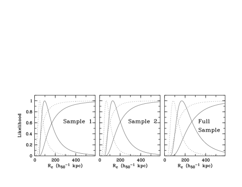
Figure 6: Likelihood function ${\cal L}(R_{\rm c})$ normalized to its peak intensity vs. cloud radius $R_{c}$, and cumulative distribution for spherical (solid line) and cylindric absorbers.

Table 4: Diameter $D$ of spherical and cylindric Ly$\alpha$ clouds in HS 1216+5032 in the redshift interval $z=1.15-1.43$ as derived from the likelihood function defined in (3). Values are in kpc and represent $2\sigma$ limits. $H_{0}=50$ km s^-1 Mpc^-1 and $q_{0}=0.5$.

$$\begin{array}[]{cccc}\hline\cr\vskip 3.0pt plus 1.0pt minus 1.0pt\cr{\rm Cloud\leavevmode\nobreak\ shape}&{\rm Sample1}&{\rm Sample2}&{\rm Sample3}\\ \vskip 3.0pt plus 1.0pt minus 1.0pt\cr\hline\cr\vskip 3.0pt plus 1.0pt minus 1.0pt\cr{\rm Spherical}&136<D<880&172<D<896&224<D<1160\\ \vskip 3.0pt plus 1.0pt minus 1.0pt\cr{\rm Cylindric}&52<D<454&86<D<460&112<D<610\\ \vskip 3.0pt plus 1.0pt minus 1.0pt\cr\hline\cr\end{array}$$

• Sample 1: Lines with $W_{0}>0.32$ Å; 2 coincidences, 4 anti-coincidences.

• Sample 2: Lines with $W_{0}>0.17$ Å; 4 coincidences, 5 anti-coincidences.

• Sample 3: Full sample: 6 coincidences, 5 anti-coincidences.

6.5 Equivalent Widths

The sample of Ly$\alpha$ lines common to both spectra gives model-independent information about the size scales of the absorbers. Figure 7 shows the rest-frame equivalent widths of lines common to both spectra and their $1\sigma$ errors, where the dashed straight line has a slope of unity. Only lines without associated metal lines are included. Note that this selection yields line-pairs with $\lambda>2620$ Å, so the influence of uncertainties in the continuum placement (e.g. due to the BAL troughs or to spectral regions with high noise level) over the equivalent-width estimates is minimized. We have included one line pair within 3 000 km s^-1 from the QSO’s redshift (A52,B49) but not the “associated system”. The dotted crosses represent line pairs for which the B line has $2.58<{\rm SNR}<3$, i.e., those ones labeled with footnote 5 in Table 3. Additionally, to illustrate the significance of the non-detections we have also included lines detected in only one spectrum, plotted against the corresponding $3\sigma$ detection limit in the other spectrum.

Most of the coincident lines are stronger in the B spectrum, which is explained by the difficulty in detecting lines in B (an additional consequence of this is that most anti-coincidences are lines in B). It can be seen that there are some significant deviations from $\Delta W_{0}=0$, even excluding the line pair within 3 000 km s^-1. For the latter such deviation would be expected, since the QSOs themselves might be an important ionizing agent in clouds next to the QSOs.

The equivalent width differences $\Delta W_{0}=|W_{0}({\rm A})-W_{0}({\rm B})|$ show no correlation with $\Delta v$. Instead, $\Delta W_{0}$ and max$(W_{0}({\rm A}),W_{0}({\rm B}))$ seem to be correlated (see Fig. 8), with larger equivalent width differences for larger equivalent widths (e.g. Fang et al. Fang (1996)). Both effects, although not statistically significant, suggest coherent structures, i.e., no “cloudlets” at similar redshifts (Charlton et al. Charlton (1995)). In conclusion, LOS A and B must sample coherent clouds showing small – but otherwise significant – density gradients on spatial scales of $\sim 80\leavevmode\nobreak\ h_{50}^{-1}$kpc, the linear separation between LOSs in this redshift range.

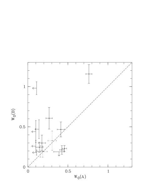
Figure 7: Rest-frame equivalent widths of Ly$\alpha$ lines common to both spectra, with ${\rm SNR}>3$, $\Delta v<100$ km s^-1, and no metal lines associated. Dotted crosses represent line pairs with $2.58<{\rm SNR}<3$. The “associated system” has not been considered. Lines detected in only one spectrum are also shown, with upper limits representing $3\sigma$ detection limits in the other spectrum.

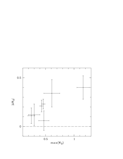
Figure 8: Absolute value of rest-frame equivalent width differences (Å) vs. $\max(W_{0}({\rm A}),W_{0}({\rm B}))$ of Ly$\alpha$ lines with ${\rm SNR}>3$, $\Delta v<100$ km s^-1, and no metal lines associated. The “associated system” has not been considered.

6.6 The $z_{a}\approx z_{e}$ Ly$\alpha$ systems in HS 1216+5032 A and B

Two $z_{a}\approx z_{e}$ Ly$\alpha$ systems are observed in the spectra of both HS 1216+5032 A and B, through the partially resolved Ly$\alpha$ lines A53, A54, A55, and B51 and B52 (see Fig. 4). The lines in A and B differ by $\Delta v_{\rm A53-B51}=-51$ km s^-1and $\Delta v_{\rm A54-B52}=-87$ km s^-1. The system in A is blueshifted by 122 km s^-1 relative to $z_{e}({\rm A})$, while the system in B is redshifted by 280 km s^-1 relative to $z_{e}({\rm B})$ (but see § 2.2). Line A55 has no clear counterpart in B. No metal lines are found associated with these systems. The total equivalent width of the A lines is larger than in B by a factor of 2.1.

The absence of highly ionized species such as N v and O vi suggests that these systems are probably not physically associated with the QSOs (e.g., Turnshek Turnshek1 (1984); Petitjean Petitjean1 (1994)). Furthermore, the small velocity differences between lines in A and B, and the fact that both systems have two line components well correlated in redshift, strongly suggest they arise in the same absorber (see also Petitjean et al. Petitjean (1998); Shaver & Robertson Shaver (1983)). If this is true, the different Ly$\alpha$ line strengths between A and B imply either characteristic transverse sizes of $\sim 80\leavevmode\nobreak\ h_{50}^{-1}$kpc or maybe even larger clouds with ionization conditions that change on such scales. The size scales are compatible with the idea that these systems arise, for example, in the very extended halo of an intervening galaxy (Weymann et al. Weymann (1979)), or in the intra-group gas of the QSO host galaxies.

If the radiation field of the QSOs is the main ionization source in the clouds giving rise to these systems (assuming the QSO pair is real), then the systems in B should be less ionized than the A ones. This is because QSO A is intrinsically more luminous than B in the ionizing continuum. Consequently, the different line strengths in A and B can also be explained if the LOSs cross regions of similar density, with LOS B probing regions with more neutral gas. Of course, the latter case does not rule out the intervening nature of these systems.

6.7 Discussion

Fang et al. (Fang (1996)) have pointed out that there seems to be a trend of larger estimated cloud sizes with increasing LOS separation $S$ (see their Fig. 5). If such a trend were real, it would imply that the scenario of uniform-sized spherical clouds is too idealized. Their data, however, are insufficient to discern whether the effect is due to non-uniform cloud size or simply non-spherical cloud geometry. The results presented in our work (slightly modified by defining a sample of lines with $W_{0}>0.40$ Å to be consistent with these authors) fit this tendency well because they add a new measurement of relatively small cloud sizes at small LOS separation. We note, however, that D’Odorico et al. (D'Odorico (1998)), who use a larger database and an improved statistical approach, find no correlation between cloud size and LOS separation. Clearly, more QSO pairs are needed that span a range in LOS separations to confirm or discard the size/separation correlation.

Here we propose that the notion of a single population of uniform-sized clouds must be revised. In fact, if Ly$\alpha$ clouds span a range of sizes between, say, a few hundred kpc to a few Mpc, then LOSs to QSO pairs with arcminute separations would be crossing not only huge and coherent structures, but also smaller clouds correlated in redshift. Further evidence for a more complicated scenario than usually assumed comes from cosmological hydrodynamic simulations made for $z=3$, which show entities of non-uniform sizes grouped along filamentary structures (e.g., Cen & Simcoe Cen (1997)). However, we recall that the situation at lower redshift can be different if such structures do evolve in size.

Size evolution of Ly$\alpha$ absorbers has not yet been observed, in part because the number of adjacent QSOs with suitable angular separations is not statistically significant, but also due to the scarce number of observations at low redshift. In particular, the present data on HS 1216+5032 ($<z>=1.3$) do not confirm the suggestion (Fang et al. Fang (1996); Dinshaw et al. Dinshaw1 (1998)) that cloud sizes increase with decreasing redshift. This result is in variance with the findings by D’Odorico et al. (D'Odorico (1998)).

Assuming that the Ly$\alpha$ absorbers are filamentary structures – modelled as cylinders of infinite length – lying perpendicular to the LOSs, our likelihood analysis leads to almost $50\%$ smaller transverse dimensions than for spherical clouds. Unfortunately, the method presented here is not capable of distinguishing between cylinders and spheres. Moreover, the information provided by two LOSs might be insufficient to make such a distinction possible, so one should use triply imaged QSOs (Crotts & Fang Crotts1 (1998)) or, even better, QSO groups (Monier et al. Monier (1999)). It is worth saying, however, that flattened structures are more able to simultaneously reproduce the requirements of neutral gas density from photoionization models and the transverse scale lengths derived from double LOSs than spherical absorbers do. Such photoionization models lead to structures with thickness-to-length ratios of $\sim 1/30$ (Rauch & Haehnelt Rauch4 (1995)). Indeed, hydrodynamical simulations in the context of hierarchical structure formation have shown that at $z\sim 3$, high density gas regions (producing $W_{0}>0.3$ Å Ly$\alpha$ absorption lines) are connected by filamentary and sheet-like structures roughly $10^{6}$ times less dense than the embedded condensations. The filaments seem to evolve slowly and still fill the Universe at $z\sim 1$ (Davé et al. Dave (1999); Riediger, Petitjean & Mücket Riediger (1998)), giving rise to the majority of strong Ly$\alpha$ lines. If this picture is correct, the requirement of different cloud populations might not be necessary to explain current observations.

New high-resolution ultraviolet observations of QSO pairs are needed. Despite technical difficulties (close QSO pairs tend to have such different observed fluxes that high dispersion spectroscopy normally leads to at least one spectrum with high noise levels) they should improve considerably our knowledge of the Ly$\alpha$-cloud geometry by (1) analyzing absorbers that produce only weak ($W_{0}\sim 0.01$ Å) lines, i.e., those surely not associated with low-brightness galaxies, and (2) testing models that consider column density distributions.

7 Summary

We have presented HST FOS spectra of the QSO pair HS 1216+5032 AB. Our results are summarized as follows:

1. Metal systems. Three strong and complex C iv absorption systems are observed in both HST spectra at $z\approx 0.72$. The velocity span along the LOSs, $\Delta v\sim 1500$ km s^-1, is large and suggests the gas where this C iv occurs might be associated with a cluster of galaxies. Differences in the line strengths suggest that, if these systems arise in coherent structures, they must have characteristic transverse sizes of $\sim 75\leavevmode\nobreak\ h_{50}^{-1}$kpc. Alternatively, the systems may be composed of a large number of cloudlets correlated in redshift.

   In the spectrum of B, a strong absorption feature at $\lambda\sim 2910$ Å is identified with two Mg ii doublets at $z=0.04$. If this identification is correct, these lines could arise in a low-redshift damped Ly$\alpha$ system.

2. The BAL systems in B: The spectrum of QSO image B shows BAL troughs by H i, C ii, C iii, N iii, N v, O vi, and possibly S iv and S vi arising in absorption systems at outflow velocities from the QSO of up to $5000$ km s^-1. The BAL troughs arise probably as a consequence of absorption by a mixture of broad and narrow components.

3. Ly$\alpha$ absorbers. Due to the redshift path blocked out by the BAL troughs in B the number of detected lines is small. Selecting lines not associated with metal lines, with $\Delta v({\rm A-B})<100$ km s^-1 and $W_{0}>0.17$ Å yields four lines common to both spectra and five lines without counterpart in the other spectrum. For $W_{0}>0.32$ Å lines the numbers are two and four, respectively. Using a maximum likelihood technique, most probably diameters for spherical clouds of $192$ and $256$ $\leavevmode\nobreak\ h_{50}^{-1}$ kpc are found for $W>0.32$ Å and $W>0.17$ Å lines, respectively. The $2\sigma$ limits derived using the cumulative distribution of the probability function are $136<D<880$ $\leavevmode\nobreak\ h_{50}^{-1}$ kpc and $172<D<896$ $\leavevmode\nobreak\ h_{50}^{-1}$ kpc for the respective samples at $<z>=1.3$. Assuming that the absorbers are filamentary structures lying perpendicular to the LOSs, transverse dimensions almost $50\%$ smaller than for spherical clouds are found. In both cases, the results of our analysis do not confirm the claim that the characteristic size of the Ly$\alpha$ absorbers increases with decreasing redshift.

   Independently of the cloud models used, we note that there are significant equivalent width differences between lines in A and B. Also, there appears to be a trend of larger equivalent width differences with increasing line strength, while no velocity differences between common lines is found. This provides evidence that the absorbers are coherent entities. The results for each line sample suggest that the absorbers must have a smooth gas density distribution, with lower density gas being more extended.

- (1) Arav, N., Becker, R. H., Laurent-Muehleisen S. A., Gregg, M. D., White, R. L., & de Kool, M. 1999a, ApJ 524, 566
- (2) Arav, N., Korista K. T., de Kool M., Junkkarinen V. T., & Begelman M. C. 1999b, ApJ 516, 27
- (3) Barlow, T. A., & Sargent W. L. W., 1997, AJ 113, 136
- (4) Bechtold, J,, Crotts, A. P. S., Duncan, R. C., & Fang, Y, 1994, ApJ 437, L83
- (5) Bergeron, J., & Stasinska, G., 1986, A&A 169, 1
- (6) Bergeron, J., & Boissé, P., 1991, A&A 243, 344
- (7) Cen, R., & Simcoe, R. A., 1997, ApJ 483, 8
- (8) Charlton, J. C., Churchill, C. W., & Linder S. M., 1995, ApJ 452, L81
- (9) Crotts, A. P. S., Bechtold, J., Fang, Y., & Duncan R. C., 1994, ApJ 437, L79
- (10) Crotts, A. P. S., & Fang, Y. 1998, ApJ 502, 16
- (11) Davé, R., Hernquist, L., Katz, N., & Weinberg, D. H., 1999, ApJ 511, 521
- (12) Dinshaw, N., Impey, C. D., Foltz, C. B., Weymann, R., & Chaffee, F. H., 1994, ApJ 437, L87
- (13) Dinshaw, N., Foltz, C. B., Impey, C. D., & Weymann, R. J., 1998, ApJ 494, 567
- (14) Dinshaw, N., Weymann, R. J., Impey, C. D., Foltz, C. B., Morris, S. L., & Ake, T., 1997, ApJ 491, 45
- (15) D’Odorico, V., Cristiani, S., D’Odorico, S., Fontana, A., Giallongo, E., & Shaver, P., 1998, A&A 339, 678
- (16) Fang, Y., Duncan, R. C., Crotts, A. P.,& Bechtold J, 1996, ApJ 462, 77
- (17) Hagen, H.-J., Groote, D., Engels, D., & Reimers, D., 1995, A&AS 111, 195
- (18) Hagen, H.-J., Hopp, U., Engels, D., & Reimers, D., 1996, A&A 308, L25
- (19) Hamann, F., Barlow, T. A., Beaver, E. A., Burbidge, E. M., Cohen, R. D., Junkkarinen, V., & Lyons, R. 1995, ApJ 443, 606
- (20) Hamann, F., Barlow, T. A., Junkkarinen, V., & Burbidge, E. M. 1997, ApJ 478, 80
- (21) Kochanek, C. S., Falco, E. E., & Muñoz, J. A., 1999, ApJ 510, 590
- (22) Kochanek, C. S. 1995, ApJ 453, 545
- (23) Lu, L. Sargent, W. L. W., Barlow, T. A., Churchill, C. W., & Vogt, S. S., 1996, ApJS 107, 475
- (24) McGill, C. 1990, MNRAS, 242, 544
- (25) Monier, E. M., Turnshek, D. A., Hazard, C., 1999, ApJ 522, 627
- (26) Petitjean, P., Rauch, M., Carswell, R. F., 1994, A&A 291, 29
- (27) Petitjean, P., Surdej, J., Smette, A., Shaver, P., Mücket, J., & Remy, M., 1998, A&A 334, L45
- (28) Rauch, M., & Haehnelt, M. G. 1995, MNRAS, 275, 76 ApJ, 467, L5
- (29) Rauch, M. 1997, in Structure and Evolution of the IGM from QSO Absorption Lines, Proc. 13th IAP Colloquium, ed. P. Petitjean, S. Charlot (Paris: Editions Frontières), 109
- (30) Riediger, R., Petitjean, P., & Mücket, J. P. 1998, A&A 329, 30
- (31) Sargent, W. L. W., Steidel, C. C., & Boksenberg, A. 1989, ApJS 69, 703
- (32) Savage, B. D., Lu, L., Bahcall, J. N., Bergeron, J., et al. 1996, ApJ 413, 116
- (33) Schneider, D. P. et al. 1993, ApJS 87, 45
- (34) Shaver, P. A., & Robertson J. G. 1992, ApJ 268, L57
- (35) Smette, A., Surdej, J., Shaver, P. A., Foltz, C. B., Chaffee, F. H., Weymann, R. J., Williams, R. E., & Magain, P. 1992, ApJ 389, 39
- (36) Smette, A., Robertson, J. G., Shaver, P. A., Reimers, D., Wisotzki, L., & Köhler, Th. 1995, A&AS 113, 199
- (37) Steidel, C. C., & Sargent W. L. W. 1992, ApJS 80, 1
- (38) Turnshek, D. A. 1984, ApJ 280, 51
- (39) Turnshek, D. A., Kopko, M., Monier, E., & Noll, D. 1996, ApJ 463, 110
- (40) Tytler, D., & Fan, X.-M. 1992, ApJS 79, 1
- (41) Verner, D. A., Barthel, P. D., & Tytler, D. 1994, A&AS 108, 287
- (42) Wampler, E. J., Chugal, N. N., & Petitjean P. 1995, ApJ 443, 586
- (43) Weymann, R. J., Williams, R. E., Peterson, B. M., & Turnshek, D. A. 1979, ApJ 234, 33
- (44) Weymann, R. J., Morris, S. L., Foltz, C. B., & Hewett, P. C. 1991, ApJ 373, 23
- (45) Weymann, R. J., Jannuzi, B. T., Lu, L., et al. 1998, ApJ 506, 1