Atomic data from the Iron Project

Abstract

Relativistic atomic structure calculations for electric dipole ($E1$), electric quadrupole ($E2$) and magnetic dipole ($M1$) transition probabilities among the first 80 fine-structure levels of Fe VI, dominated by configurations $3d^{3},3d^{2}4s$, and $3d^{2}4p$, are carried out using the Breit-Pauli version of the code SUPERSTRUCTURE. Experimental energies are used to improve the accuracy of these transition probabilities. Employing the 80-level collision-radiative (CR) model with these dipole and forbidden transition probabilities, and Iron Project R-matrix collisional data, we present a number of [Fe VI] line ratios applicable to spectral diagnostics of photoionized H II regions. It is shown that continuum fluorescent excitation needs to be considered in CR models in order to interpret the observed line ratios of optical [Fe VI] lines in planetary nebulae NGC 6741, IC 351, and NGC 7662. The analysis leads to parametrization of line ratios as function of, and as constraints on, the electron density and temperature, as well as the effective radiation temperature of the central source and a geometrical dilution factor. The spectral diagnostics may also help ascertain observational uncertainties. The method may be generally applicable to other objects with intensive background radiation fields, such as novae and active galactic nuclei. The extensive new Iron Project radiative and collisional calculations enable a consistent analysis of many line ratios for the complex iron ions.

1 Introduction

Recently a wealth of optical and UV spectra in Fe VI have been observed from gaseous nebulae and hot H II regions in general, and from hot white dwarfs (Jordan et al. 1995). Emission lines from transitions among the first 19 fine-structure levels dominated by the ground configuration $3d^{3}$ also appear in nova V 1016 Cygni (Mammano and Ciatti, 1975) and RR Telescoppii (McKenna et al. 1997). Optical spectra of [Fe VI] have been observed for many transitions in planetary Nebulae such as NGC 6741 (Hyung and Aller 1997a), NGC 7662 (Hyung and Aller 1997b), IC 351 (Feibelman et al. 1996), and others. It is therefore interesting to simulate these spectra using accurate atomic data from the Iron Project (Hummer et al. 1993) obtained using $ab~{}initio$ calculations.

Given the state-of-the-art observational accuracy of astrophysical work, it is necessary to use accurate atomic radiative and electron impact excitation (EIE) data in order to calculate accurately the intensities ratios of prominent density and temperature sensitive lines of [Fe VI]. In the collisional-radiative (hereafter CR) model, all of the level contributions are coupled together and need to be considered. Furthermore, we have recently shown (Chen and Pradhan 2000; hereafter CP00) that in addition to EIE and spontaneous radiative decay, level populations in Fe VI are significantly affected by fluorescent excitation (hereafter FLE) via a radiation backgound, typically a UV continuum. From an atomic physics point of view this requires additional physical mechanisms to be included in the atomic model in order to correctly predict the line intensities. In fact, it was demonstrated in CP00 that the observed [Fe VI] optical line ratios in the high excitation PNe NGC 6741 can not be interpreted without taking account of the FLE mechanism (as proposed by Lucy 1995; see also Bautista, Peng, and Pradhan 1996), which. depends on strong dipole allowed excitations from the ground, or low-lying levels, and cascades into the upper levels of observed transitions.

In order to implement the FLE mechanism in the CR model therefore, one needs both the forbidden and the dipole allowed transition probabilities, in addition to the EIE rate coefficients. Accurate EIE collison strengths and rate coefficients of Fe VI have recently been computed under the IP by the Ohio-State group using the $R$-matrix method. The excitation rate coefficients differ considerably from previous works (IP.XXXVII, Chen and Pradhan 1999b; hereafter CP99b). The present work has a two-fold aim: (i) to compute transition proabilities Fe VI, and (ii) to use a CR model with FLE to compute line intensity ratios as possible temperature and density diagnostics. It is further shown that, following CP00, the radiation temperature of the central source and the distance of the emission region may be determined if the FLE mechanism is operative. The extended CR model takes account of the two competing excitation mechanisms, due to electron excitation (EIE), and photon excitations (FLE).

A large number of line ratios of [Fe VI] are examined. Density and temperature diagnostics line ratios are determined and applied to interpret observational data from a sample of planetary nebulae. The spectral diagnostics developed herein should have general applications to various other astrophysical sources.

2 Atomic calculations

The EIE calculations are described in detail in CP99a,b, and compared with previous works. Below, we briefly summarise the qualitative aspects of those results. The next subsection discusses in detail the present calculations for the forbidden and allowed A-values for Fe VI.

2.1 Electron Impact Excitation of Fe VI

With the exception of two calculations two decades ago, there were no other calculations until the recent work reported in CP99a,b. It is difficult to consider the relativistic effects together with the electron correlation effects in this complex atomic system, and the coupled channel calculations necessary for such studies are very computer intensive. The two previous sources for the excitation rates of Fe VI are the non-relativistic close coupling (CC) calculations by Garstang et al. (1978) and the distorted-wave (DW) calculations by Nussbaumer and Storey (1978). Although the Garstang et al. (1978) calculations were in the CC approximation, they used a very small basis set and did not obtain the resonance structures; their results are given only for the averaged values. The Nussbaumer and Storey (1978) calculations were in the DW approximations that does not enable a treatment of resonances. Therefore neither set of calculations included resonances or the coupling effects due to higher configurations. Owing primarily to these factors we find that the earlier excitation rates of Nussbaumer and Storey are lower by up to factors of three or more when compared to the new Fe VI rates presented in CP99b.

2.2 Radiative transition probabilities

The target expansions in the present work are based on the 34-term wave function expansion for Fe VI developed by Bautista (1996) using the SUPERSTRUCTURE program in the non-relativistic calculations for photoionization cross sections of Fe V. The SUPERSTRUCTURE calculations for Fe VI were extended to include relativistic fine structure using the Breit-Pauli Hamiltonian (Eissner et al. 1974; Eissner 1998). The designations for the 80 levels (34 LS terms) dominated by the configurations $3d^{3}$, $3d^{2}4s$ and $3d^{2}4p$ and their observed energies (Sugar and Corliss, 1985), are shown in Table 1. These observed energies were used in the Hamiltonian diagonalization to obtain the R-matrix surface amplitudes in stage STGH (Berrington et al. 1995). This table also provides the key to the level indices for transitions in tabulating dipole-allowed and forbidden transition probabilities and the Maxwellian-averaged collision strengths from CP99a,b. Examining the new Breit-Pauli SUPERSTRUCTURE calculations we deduce that the computed energy values for levels 7 and 13; levels 11 and 12 in Table 1 of CP99a should be reversed given the level designations, respectively. An indication of the accuracy of the target eigenfunctions may be obtained from the calculated energy levels in Table 1 of CP99a, and from the computed length and velocity oscillator strengths for some of the dipole fine structure transitions given in their Table 2. The agreement between the length and velocity oscillator strengths is generally about 10%, an acceptable level of accuracy for a complex iron ion.

2.2.1 Dipole allowed fine-structure transitions

The weighted oscillator strength $gf$ or the Einstein $A$-coefficient for a dipole allowed fine-structure transition is proportional to the generalised line strength (Seaton 1987) defined, in either length form or velocity form, by the equations

$$S_{L}=\mid<\Psi_{j}\mid\sum^{N+1}_{k=1}z_{k}\mid\Psi_{i}>\mid^{2}$$ (1)

and

$$S_{V}=\omega^{-2}\mid\left<\Psi_{j}\mid\sum^{N+1}_{k=1}\frac{\partial}{\partial z_{k}}\mid\Psi_{i}\right>\mid^{2}$$ (2)

where $\omega$ is the incident photon energy in Ry, and $\Psi_{i}$ and $\Psi_{j}$ are the wave functions representing the initial and final states, respectively.

Using the transition energy, $E_{ij}$, between the initial and final states, $g_{i}f_{ij}$ and $A_{ji}$for this transition can be obtained from S as

$$g_{i}f_{ij}=\frac{E_{ij}}{3}S$$ (3)

and

$$A_{ji}(a.u.)=\frac{1}{2}\alpha^{3}\frac{g_{i}}{g_{j}}E_{ij}^{2}f_{ij}=2.6774\times 10^{9}(E_{j}-E_{i})^{3}S^{E1}_{ij}/g_{j}$$ (4)

where $\alpha=1/137.036$ is the fine structure constant in a.u., and $g_{i}$, $g_{j}$ are the statistical weights of the initial and final states, respectively. In terms of c.g.s unit of time,

$$A_{ji}(s^{-1})=\frac{A_{ji}(a.u.)}{\tau_{0}}$$ (5)

where $\tau_{0}=2.4191^{-17}s$ is the atomic unit of time.

We can use experimental transition energy $E_{ij}^{exp}$ to obtain refined $g_{i}f^{e}_{ij}$ and $A^{e}_{ji}$ values through

$$g_{i}f^{e}_{ij}=g_{i}f_{ij}\frac{E_{ij}^{exp}}{E_{ij}^{cal}}$$ (6)

$$A^{e}_{ji}=A_{ji}(\frac{E_{ij}^{exp}}{E_{ij}^{cal}})^{3}$$ (7)

Computed $gf_{L}$ and $gf_{V}$ values, in both the length and the velocity formulations, for 867 $E1$ (dipole allowed and intercombination) transitions within the first 80 fine structure levels are tabulated in Table 2 (a partial table is given in the text; the complete Table 2 is available electronically from the CDS library). Transition probabilities $A_{L}$ are also given in the length formulation, which is generally more accurate than the velocity formulation in the present calculations. Experimental level energies are used to improve the accuracy of the calculated $gf$ and A-values. All of these $E1$ transition probabilities of Fe VI were incorporated in the calculation of line ratios when accounting for the FLE effect by the UV continuum radiation field (details below).

2.2.2 Forbidden electric quadrupole ($E2$) and magnetic dipole ($M1$) transitions

The Breit-Pauli mode of the SUPERSTRUCTURE code was also used to calculate the $E2$ and the $M1$ transitions in Fe VI. The configuration expansion was adapted from that used to optimise the lowest 34 LS terms by Bautista (1996). The spectroscopic configurations,the correlation configurations and the scaling parameters $\lambda_{nl}$ for the Thomas-Fermi-Dirac-Amaldi type potential of orbital $nl$ are listed in Table 3 and Table 4 of CP99a. Much effort was devoted to choosing the correlation configurations to optimise the target wavefunctions, within the constraint of computational constraints associated with large memory requirements for many of the $3p$ open shell configurations. The primary criteria in this selection are the level of agreement with the observed values for (a) the level energies and fine structure splittings within the lowest LS terms, and (b) the f-values for a number of the low lying dipole allowed transitions. Another practical criterion is that the calculated $A$-values should be relatively stable with minor changes in scaling parameters.

Like the procedure used in the calculation of the dipole allowed and intercombination $E1$ $gf$-values, the experimental level energies are also used to improve the accuracy of the computed $E2$ and $M1$ transition probabilities $A^{E2}$ and $A^{M1}$, given as

$$g_{j}A^{E2}_{ji}=2.6733\times 10^{3}(E_{j}-E_{i})^{5}S^{E2}(i,j)(s^{-1})$$ (8)

and

$$g_{j}A^{M1}_{ji}=3.5644\times 10^{4}(E_{j}-E_{i})^{3}S^{M1}(i,j)(s^{-1})$$ (9)

The computed $A^{E2}$ and $A^{M1}$ for all 130 transitions among the first 19 levels are given in Table 3. The results calculated by Garstang et al. (1978) and by Nussbaumer and Storey (1978) are also given for comparison, where available. For 70 transitions in Table 3 the $A^{E2}$ are much smaller than the $A^{M1}$, by up to several orders of magnitude for some transitions. While for the other 60 transitions, $A^{E2}$ are greater than the $A^{M1}$. The computed $A^{E2}$ and $A^{M1}$ for all the other 1101 transitions within the first 80 levels are given in Table 4 (a partial table is given in the text; the complete Table 4 is available electronically from the CDS library). There are no other calculations in literature for these transitions for comparisons. There are many cases where one of the two transition probabilities is negligible, usually the $A^{E2}$. But the case of Fe VI is somewhat different from that of Fe III (Nahar and Pradhan 1996), where the $A^{E2}$ are greater than $A^{M1}$ for nearly half the total number of transitions, especially those with large excitation energies.

3 The 80-level collision radiative model with fluorescence

A CR model with 80 levels for Fe VI is employed to calculate level populations, $N_{i}$, relative to the ground level. The emitted flux per ion for transition $j\rightarrow i$, or the emissivity $\epsilon_{ji}$ (ergs cm^-3s^-1), is given by,

$$\epsilon_{ji}=N_{j}A_{ji}h\nu_{ij}$$ (10)

The line intensities ratios, for example, $\epsilon_{ji}/\epsilon_{kl}$ for transitions j-i and k-l are then calculated. A computationally efficient code to set up CR matrix in CR model is employed to solve the coupled linear equations for all levels involved (Cai and Pradhan 1993).

We can write the rate coupled equations of statistical equilibrium in CR matrix form:

$${\bf C=NeQ+A}$$ (11)

where $Ne$ is the electron density, and

$$C_{ii}=0\\ C_{ij}=q_{ij}Ne~{}~{}~{}(j>i)\\ C_{ij}=q_{ij}Ne+A_{ij}~{}~{}~{}(j<i)\\$$ (12)

In the above model, we have assumed the optically thin case. FLE by continua pumping and other pumping mechanisms are not considered in this mode. Also, the line emission photons from the tramsitions within the ions are assumed to escape directly without absorption (Case A).

In a thermal continuum radiation field of optically thick gaseous nebulae, the ion can be excited by photon pumping or de-excited by induced emission. With the FLE mechanism for excitation or de-excitation in the CR model, Eqs. [10] and [11] should be replaced by

$$C_{ij}=q_{ij}Ne+J_{ij}B_{ij}~{}~{}~{}(j>i)\\ C_{ij}=q_{ij}Ne+A_{ij}+J_{ij}B_{ij}~{}~{}~{}(j<i)\\$$ (13)

where $J_{ij}$ is the mean intensity of the continuum at the frequency for transition $i\rightarrow j$. $B_{ij}$ is the Einstein absorption coefficient or induced emission coefficients. For a blackbody radiation with effective temperature $T_{eff}$, $J_{ij}$ can be expressed as

$$J_{ij}=WF_{\nu}=W\frac{8\pi h\nu^{3}}{c^{2}}\frac{1}{e^{h\nu/kT_{eff}}-1}$$ (14)

where $\pi F_{\nu}$ is the monochromatic flux at the photosphere with an effective temperture $T_{eff}$. $W=\frac{1}{4}(\frac{R}{r})^{2}=1.27\times 10^{-16}(\frac{R_{\ast}/R_{\odot}}{r/pc})^{2}$ is the geometrical dilution factor, R and r being the radius of the photosphere and the distance between the star and the nebula, respectively. More accurate specific luminosity density function versus frequency, or the mean intensity, may be employed in ohter applications, e.g. in the synchrotron continuum pumping in the Crab nebula (Davidson & Fesen 1985; Lucy 1995).

With the notations used and explanations given above, the equation of statistical equlibrium for the kth level has the form

$$\sum_{j\neq k}(N_{j}C_{jk}-N_{k}C_{kj})=0$$ (15)

The attenuation effect in continuum intensity $J_{ij}$ has been neglected in the above rate equations, i.e. there are no optical depths along the line of observation in the nebula to the continuum radiation source. This approximation may be responsible for part of the difference between the calculated and observed line ratios as shown in Table 6 below. With this approximation, the rate coefficients $C_{ij}$ are independent of level population $N_{k}$; the rate equations are therefore linear and can be solved directly.

4 [Fe VI] line ratios: temperature and density diagnostics

Some of the salient features of the spectral diagnostics with FLE are discussed in CP00. It is shown that the line ratios can be parametrized as a function of $T_{e},N_{e},T_{eff},W(r)$. For a given subset of ($T_{e},N_{e}$) a line ratio may describe the locus of the subsets of ($T_{eff},W(r)$), which then defines (constrains) a contour of possible parameters. CP00 present 3-dimensional plots of the line ratio vs. ($T_{eff},W(r)$), for given ($T_{e},N_{e}$). While it is clear that the $T_{eff}$ or the $W(r)$ can not be determined uniquely and independently, it was found that the observed value of the line ratio cuts across the surface (double-valued function in $T_{eff},W(r)$), along the contour of likely values that lie within. The variation of the intensity ratio with effective temperature and the distance of the emitting region may constrain these two macrospopic quantities, in addition to the determination of the local electron temperature and density.

The spectral diagnostics so developed is applied to the analysis of [Fe VI] lines from planetary nebulae as described below.

4.1 Planetary Nebulae

The central stars of planetary nebulae correspond to high stellar radiation temperatures (e.g. Harman and Seaton 1966), of the order of 10⁵ K. Resonant absorption was first discussed by Seaton (1968), who pointed out the efficacy of this mechanism in line formation of [O III], in addition to electron scattering and recombination, estimated the oxygen abundance taking this into account. We might expect, a priori, that if the atomic structure of the emitting ion is subject to FLE then the PNe might be good candidates for radiative fluorescence studies in general, as shown in CP00.

In recent years, Hyung and Aller in particular have made a number of extensive spectral studies of PNe, and in nearly all of those [Fe VI] optical emission lines have been detected (Table 5). Physical conditions in some of the PNe’s are listed in Table 5. Observed line ratios are used to develop the temperature-density diagnostics for [Fe VI]. An earlier study of [Fe VI] line ratios was carried out by Nussbaumer and Storey (1978) who calculated a number of line emissivities relative to the $\lambda$ 5146 $\AA$ line. Owing to new atomic collisional and radiative data our line ratios differ significantly from the earlier work for many lines. Also, Nussbaumer and Storey (1978) did not take the FLE mechanism into account. On examination of the observed [Fe VI] lines in several PNe, we noted that the $\lambda$ 5146 $\AA$ line was mis-identified and assigned to [O I] in the PNe labeled a,c,d in Table 5 (in a private communication we confirmed the new identification with Prof. Lawrence Aller, who noted that [Fe VI] was the more likely source, particularly in NGC 6741 which is a high excitation object).

A comprehensive study of most of the possible line ratios was carried out as functions of $T_{e}$, $N_{e}$, and with and without FLE, at various radiation temperatures T_eff and dilution factors W($R_{\ast}/r)$. In Table 6 we present line ratios for lines which frequently appear in various kinds of PNe’s, with different physical conditions, with respect to the line $\lambda$ 5146$\AA$ (as in Nussbaumer and Storey 1978). The partial Table 6 given in the text contains only those line ratios for which observed values are available. The complete Table 6 (available electronically from the CDS library), gives a number of other line ratios computes in a similar manner relative to the $\lambda$ 5146$\AA$.

Line ratios are calculated with different dilution factors within the CR model in order to evaluate the influence of FLE under different conditions. The first four entries are: no FLE, FLE with $W=5\times 10^{-16},10^{-13},10^{-10}$ respectively. The Nussbaumer and Storey (1978) values are given as the fifth set of entries for comparison. Also, observational values are give in these entries (under “Obs”) for various planetary nebulae, wherever available.

4.2 NGC 6741

Observations of this high excitation nebula by [Aller et al. (1985)] and [Hyung and Aller (1997a)] show several optical [Fe VI] lines in the spectrum from the multiplet $3d^{3}\ (^{4}F-^{4}P)$ at 5177, 5278, 5335, 5425, 5427, 5485, 5631 and 5677 $\AA$ and from the $(^{4}F-^{2}G)$ at 4973 and 5146 $\AA$ for NGC 6741. The basic observational parameters, in particular the inner and the outer radii needed to estimate the distance from the central star and the dilution factor, are described in these works, and their diagnostic diagrams based on the spectra of a number of ions give $T_{e}=12500K,N_{e}=6300cm^{-3}$, and a stellar $T_{eff}=140,000K$. As the ionization potentials of Fe V and Fe VI are 75.5 eV and 100 eV respectively, compared to that of He II at 54.4 eV, Fe VI emission should stem from the fully ionized $He^{2+}$ zone, and within the inner radius, i.e. r(Fe VI) $\leq r_{in}$. With these parameters we obtain the dilution factor to be W = 10^-14; the dominant [Fe VI] emission region could be up to a factor of 3 closer to the star, with W up to 10^-13, without large variations in the results obtained.

Figs. 1 and 2 show all the line ratios for NGC 6741 (with respect to the 5146 $\AA$ line), where observational values are available (Hyung and Aller 1997a). [Fe VI] line ratios are presented as a function of several parameters, in particular with and without FLE. In all cases the FLE = 0 curve fails to correlate with the observed line ratios, and shows no dependence on N_e (an unphysical result), whereas with FLE we obtain a consistent $N_{e}\approx$ 1000-2000 cm^-3, suitable for the high ionization [Fe VI] zone. The derived N_e is somewhat lower than the N_e range 2000 - 6300 cm^-3 obtained from several ionic spectra (including [O II] and [S II]) by [Hyung and Aller (1997a)]. The total observational uncertainties cited by Hyung and Aller (1997a) are 17.6%, 19.5%, 38.9%, 15.6%, 23.2%, 25.5%, 10.2%, 14.5%, and 36.5% for 4973, 5177, 5278, 5335, 5425, 5427, 5485, 5631 and 5677 $\AA$ (with respect to the 5146 $\AA$ line), respectively (Hyung and Aller 1997a). However, an indication of the overall uncertainties may be obtained from the 1st line ratio, 4973/5146, which is independent of both T_e and N_e since both lines have the same upper level, and which therefore depends only on the ratio of the A-values and energy separations; the observed value of 1.048 agrees closely with the theoretical value of 0.964. Whereas the combined observational and theoretical uncertainties for any one line ratio can be significant, most measured line ratios (except three line ratios 5278/5146, 5427/5146 and 5677/5146 which will be analyzed in the next paragraph) yield a remarkably consistent N_e([Fe VI]) and substantiate the spectral model with FLE.

While the electron density of the [Fe VI] in NGC 6741 is determined to be $\approx$ 1000-2000 cm^-3 from most of the observational line ratios as demonstrated above, we note from Fig. 2 that three line ratios 5278/5146, 5427/5146 and 5677/5146 deviate from this N_e considerably. It is interesting to estimate the possible errors in these three observational line ratios from our theoretical method and model. Several pairs of line ratios are shown in Table 7 that have a common upper level. These line ratios depend only on the ratio of the A-values and energy differences and are independent of the detailed physical conditions in PN. They can be used as important means to determine possible, systematic errors in the observed line intensties as described below.

From the line ratio 4973/5146, independent of PN physical conditions as mentioned above, and the other five line ratios in Table 7, we conclude that the intensity of the reference line 5146 $\AA$ should be very accurate. It is very unlikely that the error for each pair of these line ratios are the same and show the same tendency. An error estimate of 6.8% for this line given by Hyung and Aller (1997a) is consistent with our justification. As such, the observed intensities of lines $\lambda\lambda$ 4973, 5177, 5335, 5425, 5485, and 5631 $\AA$ should be of high accuracy (within 20%). This conclusion is also supported by the good agreement between the two other theoretical and observational line ratios 5335/5485 and 5425/5632 shown in Table 7.

Based on these arguments, we find that the observed (‘Hamilton’) line intensity of 0.087 (Hyung and Aller 1997a) (relative to the uniform flux of I(H$\beta$)=100) for 5278 $\AA$ should be reduced by about 40% from a comparison of the line ratio 5278/5425 in Table 7. Similarly, the reported line intensity of 0.118 for the line 5427 $\AA$ should be reduced by about 70% or more, and the value 0.122 for the 5677 $\AA$ should be increased by 20% or so from the comparison of the line ratio 5427/5677 in Table 7. If our justifications for the errors in the intensities of these three lines are correct, the corresponding three line ratios shown in Fig. 2 will also yield the same and consistent N_e as do the other line ratios, particularly those in Fig. 1. It is interesting to note that the uncertainties given by Hyung and Aller (1997a) are also large (as inferred above), although the line 5427 $\AA$ could have a much higher uncertainty (intensity larger or lower).

4.3 IC 351

The physical conditions of IC 351, especially the effective temperature T_eff and the distance of PN emission region to the central white dwarf (WD), are highly uncertain. We first apply our method, as developed in CP00, to determine the appropriate T_eff and the dilution factor W(r). T_eff is thereby determined to be 80,000$\pm$10,000 K. This is considerably different from T_eff=58,100K cited by [Feibelman et al. (1996)]. It is interesting to note that the T_eff determined by our spetral method with FLE agrees with the He II Zanstra temperature, which is 85,000K according to [Preite-Martinez and Pottasch (1983)]. As pointed out by [Preite-Martinez and Pottasch (1983)], different methods (Zanstra method, color temperature and energy balance method, etc.) used to determine the effective temperature of PN remain discrepant; but the He II Zanstra method is applicable to optically thick PN’s. With the T_eff as above, we obtain the dilution factor W(r) to be 10^-13 – 10^-14.

After determining T_eff and W(r), the same method as used in NGC 6741 is applied to determine the electron density N_e of the [Fe VI] emission nebula in IC 351, and possible errors in the observed line intensities. There are 7 observational line ratios for IC 351 as shown in Figs. 3 and 4; but we calculated the same 8 line ratios theoretically as for NGC 6741. The only reported uncertainty for a line ratio given by [Feibelman et al. (1996)] is 36.6% for the pair 5335/5146 (Fig. 3). When we look into the comparison of line ratios for IC 351 from Table 7 (pairs of line ratios with common upper level), we find that the agreement of 4973/5146 is good ($\approx$ 10%) between calculation and observation. This establishes that the intensities of both the 4973 and 5146 $\AA$ lines should be highly accurate ($\approx$ 10%). The diffierence is 26% for 5427/5677 (Fig. 4), 92% for 5335/5485 (Fig. 3), and 175% for 5278/5425 (Fig. 4). From these differences, and Figs. 3 and 4, we could estimate the possible errors in some of the observed lines: line 5485 $\AA$ should be reduced by 60%; line 5336 $\AA$ increased by 20%; line 5278 $\AA$ reduced by 175%. The intensity of the line 5425 $\AA$ is accurate. From these 4 line ratios, N_e is determined to be $\approx$ 1,000 cm^-3. Using this N_e and Fig. 4, and the comparison of the line ratio 5427/5677 in Table 7, the possible errors in the intensities of the other 3 observed lines can be deduced as follows: line 5427 $\AA$ should be reduced by 80%; line 5677 $\AA$ reduced by 40%; and line 5177 $\AA$ increased by 20%. In summary, the above error analysis is based on Table 7 and the theoretically computed line ratios reported in this work (Figs. 3 and 4).

4.4 NGC 7662

Finally we apply our spectral diagnostics, and the same procedures used above, to NGC 7662. In this PN, the effective temperature T_eff and emission region distance to the central star seem to have been determined within low uncertainties. Hence, we adopt here T_eff=105,000 K and W=10^-14 ([Hyung and Aller (1997b)]) in our present calculation and the results are shown in Figs. 5 and 6. However, the observational uncertainties in line intensities are even larger than those in [Feibelman et al. (1996)] as shown from both the rms uncertainties given in [Hyung and Aller (1997b)] and our detailed spectral analysis by using the method developed by Chen and Pradhan (2000). The more complex problem is that our reference line 5146 $\AA$ has very large observational uncertainty in NGC 7662, in contrast to NGC 6741 or IC 351. Therefore we need to determine the uncertainty of this reference line first, before the general spectral diagonosis of NGC 7662 including N_e can proceed.

That the uncertainty in observational intensity of line 5146 $\AA$ is large can be established from the comparison of the physical-condition-independent line ratio 4973/5146 shown in Table 7 for NGC 7662. We also have some supplemental evidence to support this conclusion. First, after some analysis, we find the observed intensity of line 5425 $\AA$ to be very accurate; at most it is too high by 5-10%. This is also consistent with the rms uncertainty given by [Hyung and Aller (1997b)], which is remarkbly low at 3.9%. Second, we could establish that the observed intensities for lines 5335 and 5177 $\AA$ are also very accurate (within 10%) by using our procedures as described above. It is very likely that only the 5335 $\AA$ line intensity needs to be increased by 5%, and the line 5177 $\AA$ intensity decreased by 5%. To further confirm our justification, we plot a new line ratio 5177/5335 in Fig. 7, which the leads to a reasonable determination of N_e. In all the above arguments, we have a consistent spectral analysis from the line ratios of 5335/5146, 5177/5146 and 5425/5146 as shown in Figs. 5 and 6, as well as the line ratio 5177/5335 in Fig. 7. As such, we conclude that: (1) the observed intensity of line 5146 should be inreased by 80%. (the rms given in [Hyung and Aller (1997b)] is 21.7%); (2) the electron density of the [Fe VI] emission region is N${}_{e}\approx$3,000 cm^-3. For this PN, we can then deduce the possible observational errors in the other lines comparing the line ratios 5335/5485 and 5425/5631 shown in Table 7. We find that the observed intensity of the line 5485 $\AA$ should be decreased by 35%; and that of line 5631 $\AA$ increased by 60%. Finally, to make the observational line ratio 5677/5146 consistent with the physical conditions including N_e determined above by all the other line ratios, the observed intensity of the line 5677 $\AA$ should be increased by 110% (the rms uncertainty given by [Hyung and Aller (1997b)] is 20.3%).

5 Conclusion and discussion

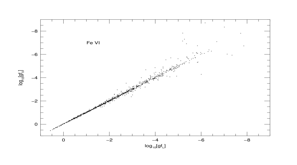
Figure 8: Comparison of Length vs. Velocity gf-values for 867 dipole allowed and intercombination $E1$ transitions in Fe VI.

An extensive calculation of fine structure transition probabilities of Fe VI is presented for the allowed $E1$ and the forbidden $E2$, $M1$ transitions. An indication of the uncertainties in the computed gf-values is given in the plot of length $gf_{L}$ vs. the velocity $gf_{V}$ for 867 $E1$ transitions computed in this work (Fig. 8). It shows an agreement at about 10% level for most of the transitions, with no more than about 5% of the transitions lying outside that range even for gf-values less than 10^-4.

Combined with previously calculated data for electron impact excitation, a 80-level CR spectral model for line ratios diagnostics is used to predict the effect of collisional and fluorescent excitation (FLE) in planetary nebulae. An illustrative and limited analysis of line ratios is carried out as an example of the use of the atomic data and the model proposed herein. Some of the diagnostics procedures developed earlier by Chen and Pradhan (2000, CP00) are employed to analyse observed line intensties from three planetary nebulae: NGC 6741, IC 351 and NGC 7662. The detailed model and analysis yields a consistent set of diagnostics, for example, for the electron density and effective temperature of the source. It shows that fluorescence effects should be included in CR models of these objects. The method may be used to determine the physical conditions in PN, especially when it is difficult to do so by other methods. For example, we have determined, within certain error limits, both the effective temperature and the emission region distance (via a dilution factor) for IC 351. By combining the line ratios that are independent of the physical conditions of PN (like cases in Table 5), and our method, we are able to estimate possible errors in the observed intensities, both individually and in term of consistency among the set of observed lines. It is expected that the method and procedures described in this paper would be generally applicable to spectral diagnostis of other radiative plasma sources, such as novae and AGN.

Finally, some possible uncertainties in our model and procedure, as employed in the present calculations, are as follows. 1) Static conditions are assumed in the CR model, independent of photoionization eqilibrium in the [Fe VI] regions of PN’s. Because [Fe VI] region is almost the highest ionization state in PN’s considered here, this assumption should not carry a large uncertainty. 2) We have assumed inherently in our procedures that there are nearly constant N$e$ and T$e$ in [Fe VI] regions. This assumption is not entirely true because both N$e$ and T$e$ are a function of the distance from the central star to the [Fe VI] emission region. However, according to 1), if photoionization equilibrium prevails then there should not be large variations in N$e$ and T$e$. 3) The radiation field should in principle simulate the ionizing stellar radiation. A further refinement of the model proposed herein would be (a) to include a radiation field with proper allowance for the Helium and Hydrogen opacities in various ionization and excitation steps, and (b) in addition to the radiation flux from the central star, resonance fluorescence from H I and He II Ly$\alpha$ should be considered in the model. However as noted earlier, Fe VI is likely to be in the fully ionized He III zone, and therefore not greatly susceptible to the effects. 4) Even though the most advanced R-matrix codes are employed in generating atomic data, the atomic data still have some uncertainties, estimated at about 10–20%.

All data tables are available electronically from the CDS, or via ftp from the authors at: chen@astronomy.ohio-state.edu.

Table 1: The 80 fine structure levels corresponding to the 34 $LS$ terms included in the calculations and their observed energies (Ry) in Fe VI (Sugar and Corliss, 1985).

i	Term		2J	Energy		i	Term		2J	Energy
1	3d3	4F	3	0.0		41	3d${}^{2}(^{3}$F)4p	4Fo	5	3.101443
2			5	0.004659		42			7	3.110750
3			7	0.010829		43			9	3.120492
4			9	0.018231		44	3d${}^{2}(^{3}$F)4p	2Fo	5	3.121742
5	3d3	4P	1	0.170756		45			7	3.131189
6			3	0.172612		46	3d${}^{2}(^{3}$F)4p	4Do	1	3.131290
7			5	0.178707		47			3	3.127568
8	3d3	2G	7	0.187870		48			5	3.137250
9			9	0.194237		49			7	3.147723
10	3d3	2P	1	0.241445		50	3d${}^{2}(^{3}$F)4p	2Do	3	3.140706
11			3	0.238888		51			5	3.152138
12	3d3	${}^{2}{\rm D}2$	3	0.260877		52	3d${}^{2}(^{3}$F)4p	2Go	7	3.179977
13			5	0.259568		53			9	3.189597
14	3d3	2H	9	0.261755		54	3d${}^{2}(^{3}$P)4p	2So	1	3.205891
15			11	0.266116		55	3d${}^{2}(^{3}$P)4p	4So	3	3.240986
16	3d3	2F	5	0.424684		56	3d${}^{2}(^{1}$D)4p	2Po	1	3.272354
17			7	0.421163		57			3	3.260106
18	3d3	2D$1$	3	0.656558		58	3d${}^{2}(^{1}$D)4p	2Fo	5	3.265386
19			5	0.653448		59			7	3.279505
20	3d${}^{2}(^{3}$F)4s	4F	3	2.386075		60	3d${}^{2}(^{3}$P)4p	4Do	1	3.275057
21			5	2.390877		61			3	3.278569
22			7	2.397871		62			5	3.287005
23			9	2.406823		63			7	3.301248
24	3d${}^{2}(^{3}$F)4s	2F	5	2.452586		64	3d${}^{2}(^{1}$D)4p	2Do	3	3.297495
25			7	2.466551		65			5	3.304281
26	3d${}^{2}(^{1}$D)4s	2D	3	2.562646		66	3d${}^{2}(^{3}$P)4p	4Po	1	3.316518
27			5	2.559763		67			3	3.320593
28	3d${}^{2}(^{3}$P)4s	4P	1	2.565008		68			5	3.330627
29			3	2.570092		69	3d${}^{2}(^{1}$G)4p	2Go	7	3.326827
30			5	2.578448		70			9	3.328555
31	3d${}^{2}(^{3}$P)4s	2P	1	2.623713		71	3d${}^{2}(^{3}$P)4p	2Do	3	3.376592
32			3	2.630266		72			5	3.376970
33	3d${}^{2}(^{1}$G)4s	2G	7	2.663908		73	3d${}^{2}(^{1}$G)4p	2Ho	9	3.390785
34			9	2.663752		74			11	3.405461
35	3d${}^{2}(^{1}$S)4s	2S	1	3.065870		75	3d${}^{2}(^{3}$P)4p	2Po	1	3.408944
36	3d${}^{2}(^{3}$F)4p	4Go	5	3.082420		76			3	3.412018
37			7	3.093542		77	3d${}^{2}(^{1}$G)4p	2Fo	5	3.454410
38			9	3.106829		78			7	3.444151
39			11	3.123191		79	3d${}^{2}(^{1}$S)4p	2Po	1	3.719860
40	3d${}^{2}(^{3}$F)4p	4Fo	3	3.094115		80			3	3.739745

Table 2: Partial Table 2 (complete table available electronically from CDS). Weighted dipole allowed $E1$ oscillator strengths $gf_{L}$, $gf_{V}$ in the length and velocity formulations, and the Einstein A-coefficients $A_{L}$ in the length formulation.

i	j	$gf_{L}$	$gf_{V}$	$A_{L}$	i	j	$gf_{L}$	$gf_{V}$	$A_{L}$
36	1	9.34e-02	9.68e-02	1.19e+09	80	2	9.64e-06	9.10e-06	2.70e+05
40	1	4.64e-01	4.68e-01	8.92e+09	36	3	2.91e-04	2.88e-04	3.68e+06
41	1	9.82e-02	9.85e-02	1.26e+09	37	3	2.14e-04	2.67e-04	2.04e+06
44	1	2.43e-03	2.50e-03	3.17e+07	38	3	1.75e-01	1.80e-01	1.34e+09
46	1	2.57e-01	2.55e-01	1.01e+10	41	3	1.05e-01	1.05e-01	1.34e+09
47	1	2.88e-02	2.89e-02	5.66e+08	42	3	9.02e-01	9.05e-01	8.71e+09
48	1	8.98e-04	8.83e-04	1.18e+07	43	3	8.20e-02	8.14e-02	6.37e+08
50	1	5.48e-02	5.40e-02	1.09e+09	44	3	8.66e-02	8.58e-02	1.12e+09
51	1	2.56e-03	2.50e-03	3.40e+07	45	3	2.86e-02	2.91e-02	2.80e+08
54	1	1.82e-06	1.86e-06	7.49e+04	48	3	5.06e-01	5.01e-01	6.62e+09
55	1	1.90e-08	1.54e-08	4.01e+02	49	3	3.99e-02	3.90e-02	3.95e+08
56	1	5.62e-03	5.89e-03	2.42e+08	51	3	8.14e-02	8.18e-02	1.07e+09
57	1	1.22e-04	1.29e-04	2.61e+06	52	3	6.25e-04	5.87e-04	6.30e+06
58	1	1.12e-04	1.09e-04	1.59e+06	53	3	1.30e-03	1.17e-03	1.06e+07
60	1	6.74e-02	7.11e-02	2.90e+09	58	3	1.12e-02	1.16e-02	1.58e+08
61	1	2.92e-02	3.06e-02	6.29e+08	59	3	6.04e-03	6.33e-03	6.48e+07
62	1	2.05e-03	2.14e-03	2.97e+07	62	3	1.71e-01	1.77e-01	2.45e+09
64	1	4.64e-04	4.80e-04	1.01e+07	63	3	2.73e-02	2.80e-02	2.97e+08
65	1	5.92e-05	5.99e-05	8.65e+05	65	3	3.28e-03	3.35e-03	4.77e+07
66	1	2.69e-05	2.67e-05	1.19e+06	68	3	1.32e-04	1.28e-04	1.95e+06
67	1	2.30e-05	2.23e-05	5.09e+05	69	3	9.30e-05	8.67e-05	1.03e+06
68	1	9.37e-07	8.67e-07	1.39e+04	70	3	1.45e-06	1.80e-07	1.28e+04
71	1	1.64e-04	1.37e-04	3.74e+06	72	3	2.46e-04	1.83e-04	3.74e+06
72	1	2.17e-05	1.86e-05	3.32e+05	73	3	2.64e-06	2.50e-06	2.42e+04
75	1	2.27e-05	1.54e-05	1.06e+06	77	3	1.38e-05	1.58e-05	2.19e+05
76	1	1.93e-06	1.28e-06	4.50e+04	78	3	7.28e-07	8.26e-07	8.62e+03
77	1	1.51e-05	1.87e-05	2.42e+05	37	4	8.83e-04	8.95e-04	8.38e+06
79	1	1.30e-05	1.26e-05	7.22e+05	38	4	1.59e-03	1.52e-03	1.22e+07
80	1	2.25e-06	2.15e-06	6.33e+04	39	4	1.86e-01	1.90e-01	1.20e+09
36	2	2.29e-03	2.47e-03	2.90e+07	42	4	7.97e-02	8.01e-02	7.66e+08
37	2	1.36e-01	1.41e-01	1.31e+09	43	4	1.29e+0	1.29e+0	1.00e+10
40	2	8.40e-02	8.49e-02	1.61e+09	45	4	3.29e-01	3.28e-01	3.20e+09
41	2	6.24e-01	6.27e-01	8.01e+09	49	4	6.18e-01	6.10e-01	6.07e+09
42	2	1.20e-01	1.19e-01	1.16e+09	52	4	8.53e-05	8.03e-05	8.57e+05
44	2	5.67e-03	5.86e-03	7.37e+07	53	4	4.35e-03	4.02e-03	3.52e+07
45	2	3.71e-03	3.76e-03	3.64e+07	59	4	5.10e-02	5.22e-02	5.45e+08
47	2	3.04e-01	3.01e-01	5.96e+09	63	4	2.30e-01	2.36e-01	2.49e+09
48	2	6.17e-02	6.10e-02	8.10e+08	69	4	3.62e-04	3.81e-04	3.97e+06
49	2	3.61e-04	3.41e-04	3.58e+06	70	4	5.33e-05	4.02e-05	4.70e+05
50	2	1.34e-01	1.34e-01	2.65e+09	73	4	2.09e-07	8.11e-08	1.91e+03
51	2	2.82e-02	2.79e-02	3.74e+08	74	4	1.18e-05	1.07e-05	9.04e+04
52	2	5.53e-04	4.96e-04	5.60e+06	78	4	1.12e-04	1.21e-04	1.32e+06
55	2	4.58e-07	4.10e-07	9.63e+03	40	5	8.03e-04	7.85e-04	1.38e+07
57	2	5.81e-04	6.07e-04	1.24e+07	46	5	1.14e-01	1.09e-01	4.03e+09
58	2	2.26e-03	2.43e-03	3.21e+07	47	5	8.80e-02	8.41e-02	1.54e+09
59	2	2.86e-04	2.88e-04	3.08e+06	50	5	2.53e-02	2.40e-02	4.48e+08
61	2	1.17e-01	1.22e-01	2.51e+09	54	5	1.56e-03	1.57e-03	5.78e+07
62	2	3.70e-02	3.84e-02	5.33e+08	55	5	1.66e-01	1.67e-01	3.15e+09
63	2	1.42e-03	1.47e-03	1.55e+07	56	5	1.88e-03	1.90e-03	7.28e+07
64	2	8.48e-04	8.65e-04	1.85e+07	57	5	5.31e-03	5.48e-03	1.02e+08
65	2	9.55e-04	9.84e-04	1.39e+07	60	5	2.36e-02	2.32e-02	9.15e+08
67	2	1.22e-04	1.21e-04	2.70e+06	61	5	2.81e-02	2.77e-02	5.46e+08
68	2	1.99e-05	1.81e-05	2.94e+05	64	5	1.97e-03	1.97e-03	3.88e+07
69	2	3.84e-06	2.14e-06	4.26e+04	66	5	1.95e-02	1.95e-02	7.75e+08
71	2	7.81e-05	5.55e-05	1.78e+06	67	5	8.78e-02	8.79e-02	1.75e+09
72	2	1.82e-04	1.48e-04	2.77e+06	71	5	2.20e-04	2.10e-04	4.55e+06
76	2	1.63e-05	1.15e-05	3.81e+05	75	5	3.78e-04	3.79e-04	1.59e+07
77	2	1.80e-06	1.96e-06	2.87e+04	76	5	4.32e-05	2.90e-05	9.11e+05
78	2	1.07e-05	1.33e-05	1.27e+05	79	5	2.11e-05	1.94e-05	1.07e+06

Table 3: Comparison of the electric quadrupole ($E2$) and magnetic dipole ($M1$) transition probabilities between the first 19 levels of Fe VI in $s^{-1}$ among the present calculation by SUPERSTRUCTURE, calculation by Garstang $et~{}al.$ (1978) and calculation by Nussbaumer and Storey (1978).

transition		Present		Garstang $et~{}al.$		NS
i	j	E2	M1	E2	M1	E2	M1
2	1	5.13e-11	5.76e-3	0.0	5.7e-3	4.97-11	5.74-3
5	1	6.04e-2	2.01e-4	8.3e-2	8.0e-5	5.97-2	3.31-4
6	1	1.27e-2	3.40e-3	1.7e-2	1.2e-3	1.26e-2	4.05e-3
7	1	7.15e-4	2.15e-4	1.0e-3	9.0e-5	7.04e-4	2.66e-4
8	1	1.90e-5	0.0	1.4e-5	0.0	1.66-5
10	1	1.99e-3	1.54e-3	7.0e-3	7.3e-4	1.54e-3	1.99e-3
11	1	6.88e-4	3.70e-1	2.8e-3	1.19e-1	5.40e-4	3.56e-1
12	1	3.84e-4	3.77e-1	6.6e-4	4.01e-1	2.67e-4	3.86e-1
13	1	5.71e-7	4.97e-2	2.8e-6	3.36e-2	9.53e-7	4.34e-2
16	1	4.62e-3	1.97e-1			4.53e-3	2.23e-1
17	1	6.60e-4	0.0			6.55e-4
18	1	3.69e-3	8.60e-2			4.14e-3	1.26e-1
19	1	6.35e-4	4.97e-3			6.30e-4	9.44e-3
3	2	2.03e-10	1.34e-2	0.0	1.3e-2	1.99e-10	1.34e-2
4	2	6.46e-10	0.0
5	2	3.47e-2	0.0	4.85e-2	0.0	3.42e-2
6	2	3.35e-2	1.97e-3	4.59e-2	6e-4	3.32e-2	1.78e-3
7	2	5.69e-3	9.87e-4	7.9e-3	4.2e-4	5.63e-3	1.36e-3
8	2	1.63e-6	2.04e-1	1.6e-5	1.73e-1	1.74e-6	2.44e-1
9	2	6.00e-6	0.0	2e-6	0.0	4.71e-6
10	2	3.19e-3	0.0	1.5e-3	0.0	2.75e-3
11	2	3.39e-3	5.98e-1	6.4e-3	1.84e-1	2.78e-3	5.75e-1
12	2	7.96e-4	7.82e-1	1.2e-3	7.1e-1	5.37e-4	7.30e-1
13	2	2.95e-5	1.44e-1	2.1e-7	9.5e-2	2.79e-5	1.39e-1
14	2	2.59e-5	0.0	2.5e-5	0.0	2.70e-5
16	2	9.77e-4	2.73e-2			1.09e-3	3.08e-2
17	2	1.90e-3	8.39e-2			1.70e-3	1.01e-1
18	2	2.77e-6	1.81e-1			1.21e-5	2.51e-1
19	2	2.05e-3	1.53e-2			2.11e-3	2.39e-2
4	3	3.66e-10	1.44e-2	0.0	1.4e-2	3.59e-10	1.45e-2
6	3	3.86e-2	0.0	5.4e-2	0.0	3.84e-2
7	3	2.12e-2	2.39e-3	2.94e-2	9e-4	2.11e-2	2.63e-3
8	3	1.83e-5	2.19e-1	1.2e-5	1.85e-1	2.02e-5	2.61e-1
9	3	2.02e-6	2.20e-1	3.1e-5	1.86e-1	1.96e-6	2.51e-1
11	3	4.95e-3	0.0	6.1e-3	0.0	4.14e-3
12	3	2.18e-3	0.0	5.3e-4	0.0	1.71e-3
13	3	3.82e-4	1.12e+0	5e-5	7.29e-1	3.41e-4	1.07e+0
14	3	6.41e-5	2.20e-3	1.6e-5	4.3e-3	7.12e-5	4.12e-3
15	3	1.83e-5	0.0	5.0e-5	0.0	1.94e-5
16	3	9.55e-4	3.57e-2			1.06e-3	3.78e-2
17	3	4.11e-4	1.49e-2			5.97e-4	1.70e-2
18	3	1.30e-2	0.0			1.57e-2
19	3	4.04e-3	1.64e-1			4.94e-3	2.45e-1
7	4	5.28e-2	0.0	7.3e-2	0.0	5.23e-2
8	4	4.06e-6	1.26e-2	8.2e-6	1.1e-2	4.29e-6	1.34e-2
9	4	7.96e-5	5.39e-1	7.8e-5	4.55e-1	8.62e-5	6.24e-1
13	4	7.74e-4	0.0	5.1e-4	0.0	6.12e-4
14	4	5.55e-6	3.35e-3	2.3e-5	7.8e-3	4.63e-6	6.86e-3
15	4	1.56e-4	6.73e-4	1.9e-4	5.7e-4	1.68e-4	1.01e-3
16	4	1.60e-4	0.0			2.04e-4
17	4	4.27e-3	2.17e-1			5.01e-3	2.56e-1
19	4	5.55e-2	0.0			6.41e-2
6	5	6.56e-13	1.86e-4	0.0	1.85e-4	6.64e-13	1.87e-4
7	5	5.71e-9	0.0
10	5	0.0	4.42e-1	0.0	3.3e-1		3.76e-1
11	5	6.09e-7	1.10e-1	2e-7	8.1e-2	4.88e-7	9.29e-2
12	5	3.67e-7	2.08e-2	1.26e-5	1.3e-3	1.71e-7	1.52e-2
13	5	3.22e-7	0.0	5.7e-6	0.0	2.84e-7
16	5	8.51e-4	0.0			5.80e-4

Table 3. continued

transition		Present		Garstang $et~{}al.$		NS
i	j	E2	M1	E2	M1	E2	M1
18	5	3.83e-2	1.26e-1			2.99e-2	1.37e-1
19	5	9.70e-3	0.0			7.16e-3
7	6	2.08e-9	4.70e-3	0.0	4.6e-3	2.09e-9	4.73e-3
10	6	1.46e-7	9.14e-6	1.5e-6	3.6e-5	2.21e-7	1.76e-5
11	6	3.61e-9	2.56e-1	9.5e-6	1.7e-1	1.69e-8	2.13e-1
12	6	1.00e-5	1.02e-2	5.4e-6	7.4e-4	8.43e-6	6.67e-3
13	6	7.01e-7	2.19e-3	5.4e-5	1.8e-3	5.06e-7	2.27e-3
16	6	1.30e-6	5.25e-4			2.13e-8	1.04e-3
17	6	3.04e-3	0.0			2.15e-3
18	6	1.05e-1	4.73e-1			8.08e-2	5.20e-1
19	6	1.02e-1	2.20e-1			7.71e-2	2.41e-1
8	7	4.85e-13	1.12e-10
10	7	2.97e-6	0.0	1.0e-5	0.0	2.45e-6
11	7	5.13e-6	1.14e-1	1.5e-5	1.19e-1	4.17e-6	1.00e-1
12	7	1.31e-6	2.19e-1	3.6e-6	7.4e-2	9.72e-7	1.76e-1
13	7	5.45e-6	7.98e-2	3.7e-6	4.3e-2	4.33e-6	6.71e-2
14	7	1.76e-9	0.0
16	7	7.10e-5	2.32e-3			6.11e-5	5.47e-3
17	7	3.12e-4	2.11e-4			2.69e-4	4.95e-4
18	7	8.14e-4	1.06e-1			7.99e-4	1.23e-1
19	7	1.49e-3	1.30e+0			1.18e-3	1.41e+0
9	8	1.41e-12	4.03e-3	0.0	4e-3	1.71e-13	4.01e-3
11	8	1.12e-5	0.0	4.9e-6	0.0	7.85e-6
12	8	6.73e-5	0.0	9.3e-5	0.0	5.13e-5
13	8	5.80e-6	2.08e-6	9.6e-6	9e-6	3.89e-6	1.06e-5
14	8	1.82e-4	8.33e-2	1.9e-4	1.38e-1	1.59e-4	1.24e-1
15	8	5.32e-6	0.0	1.7e-5	0.0	4.28e-6
16	8	1.47e-1	1.35e-1			1.49e-1	1.49e-1
17	8	1.24e-2	2.29e-1			1.24e-2	2.53e-1
18	8	1.25e+01	0.0			1.18e+1
19	8	9.45e-1	1.99e-3			9.07e-1	2.23e-3
13	9	5.83e-5	0.0	5.9e-5	0.0	4.08e-5
14	9	2.32e-5	1.43e-1	0.0	2.35e-1	2.53e-5	2.11e-1
15	9	1.35e-4	7.84e-2	2.2e-4	1.29e-1	1.13e-4	1.16e-1
16	9	7.32e-5	0.0			2.06e-5
17	9	1.24e-1	1.07e-1			1.26e-1	1.17e-1
19	9	1.07e+1	0.0			1.00e+1
11	10	1.32e-12	2.19e-4	0.0	3.2e-4	1.21e-12	2.30e-4
12	10	3.15e-7	4.08e-2	4.0e-7	1.18e-2	2.94e-7	3.80e-2
13	10	7.59e-8	0.0	1e-7	0.0
16	10	1.63e-2	0.0			1.41e-2
18	10	1.54e+0	5.98e-3			1.43e+0	2.21e-3
19	10	6.28e-1	0.0			5.87e-1
12	11	5.15e-8	1.04e-1	3e-7	6.56e-2	5.89e-8	1.02e-1
13	11	8.66e-8	5.96e-2	8e-7	2.6e-2	1.10e-7	5.56e-2
16	11	1.05e-2	6.60e-3			1.07e-2	8.08e-3
17	11	2.26e-2	0.0			2.13e-2
18	11	2.11e+0	2.14e-2			2.08e+0	1.08e-2
19	11	6.72e-1	2.98e-1			6.63e-1	3.47e-1
13	12	7.95e-13	2.54e-5	0.0	3.4e-5	6.88e-13	2.70e-5
16	12	2.19e-2	5.41e-3			2.30e-2	7.71e-3
17	12	9.32e-4	0.0			4.44e-4
18	12	5.98e-2	9.58e-3			2.56e-2	3.81e-3
19	12	1.58e+0	2.69e-1			1.46e+0	3.09e-1
14	13	6.89e-15	0.0
16	13	7.25e-3	2.75e-2			7.66e-3	3.63e-2
17	13	2.92e-2	1.02e-2			3.10e-2	1.36e-2
18	13	2.73e-1	7.48e-1			2.96e-1	8.64e-1
19	13	5.79e-1	4.77e-3			6.22e-1	4.80e-3
15	14	5.22e-11	1.33e-3	0.0	1.3e-3	5.33e-11	1.32e-3
16	14	7.02e-2	0.0			6.78e-2
17	14	1.20e-3	5.00e-4			8.85e-4	8.13e-4

Table 3. continued

transition		Present		Garstang $et~{}al.$		NS
i	j	E2	M1	E2	M1	E2	M1
19	14	1.19e-1	0.0			1.50e-1
17	15	5.18e-2	0.0			4.99e-2
17	16	3.12e-12	8.88e-4			2.88e-12	8.86e-4
18	16	5.14e-1	3.95e-1			4.67e-1	3.72e-1
19	16	9.09e-2	6.41e-1			8.26e-2	6.01e-1
18	17	1.05e-1	0.0			9.67e-2
19	17	5.24e-1	3.73e-1			4.75e-1	3.50e-1
19	18	7.24e-11	6.42e-4			6.68e-11	6.41e-4

Table 4: Partial Table 4 (complete table available from CDS). Electric quadrupole ($E2$) and magnetic dipole ($M1$) transition probabilities between the first 80 levels of Fe VI in $s^{-1}$ in the present calculation by SUPERSTRUCTURE.

i	j	E2	M1	i	j	E2	M1	i	j	E2	M1	i	j	E2	M1
20	1	4.12e+4	6.84e-6	30	5	9.36e+3	0.0	26	10	8.54e+3	5.52e-5	33	14	6.87e+4	2.90e-3
21	1	2.68e+4	2.50e-5	31	5	0.0	2.86e-2	27	10	3.32e+3	0.0	34	14	1.68e+3	5.30e-3
22	1	2.51e+3	0.0	32	5	1.12e+2	6.88e-3	28	10	0.0	2.53e-4	22	15	1.19e+2	0.0
24	1	2.63e-1	7.50e-4	35	5	0.0	1.97e-4	29	10	8.11e+3	4.29e-6	23	15	1.49e+1	9.31e-7
25	1	3.57e-2	0.0	20	6	4.29e+3	3.09e-8	30	10	4.02e+3	0.0	25	15	5.88e+4	0.0
26	1	4.13e+3	8.11e-4	21	6	8.71e+3	1.42e-6	31	10	0.0	2.34e-4	33	15	2.31e+3	0.0
27	1	1.48e+2	7.62e-5	22	6	9.26e+3	0.0	32	10	1.07e+4	7.71e-5	34	15	6.46e+4	2.90e-3
28	1	4.20e+4	1.93e-6	24	6	1.64e+2	1.77e-7	35	10	0.0	3.08e-2	20	16	7.74e+0	1.87e-3
29	1	4.24e+3	9.91e-4	25	6	8.96e+1	0.0	20	11	2.65e+1	1.39e-4	21	16	2.15e+0	2.14e-4
30	1	2.52e+2	6.16e-5	26	6	1.03e+4	2.65e-4	21	11	7.38e+1	1.50e-4	22	16	1.96e+0	3.00e-4
31	1	3.18e+0	8.46e-6	27	6	1.35e+4	7.67e-4	22	11	1.33e+2	0.0	23	16	1.27e-1	0.0
32	1	8.58e-1	1.28e-8	28	6	5.62e+3	2.54e-3	24	11	1.74e+4	1.13e-4	24	16	4.36e+3	7.11e-6
33	1	1.58e+0	0.0	29	6	7.95e+3	4.01e-4	25	11	1.47e+3	0.0	25	16	4.18e+2	2.74e-3
35	1	1.71e+1	4.03e-8	30	6	1.09e+4	2.04e-3	26	11	9.61e+2	3.38e-4	26	16	5.33e+3	2.20e-4
20	2	3.94e+4	6.70e-5	31	6	1.01e+3	5.91e-6	27	11	1.21e+4	6.87e-4	27	16	1.29e+3	4.16e-4
21	2	2.23e+4	2.14e-6	32	6	2.00e+2	1.28e-2	28	11	1.44e+2	4.15e-5	28	16	3.22e+1	0.0
22	2	2.64e+4	5.43e-5	33	6	5.07e+0	0.0	29	11	5.10e+1	1.27e-4	29	16	4.78e+3	2.44e-4
23	2	1.58e+3	0.0	35	6	6.08e+1	5.35e-4	30	11	1.44e+4	6.58e-5	30	16	7.93e+2	2.95e-4
24	2	8.11e+1	1.59e-4	20	7	3.03e+2	1.62e-7	31	11	3.62e+4	1.53e-3	31	16	7.47e+4	0.0
25	2	8.71e+0	2.89e-4	21	7	1.82e+3	2.99e-8	32	11	8.82e+2	4.32e-3	32	16	1.05e+4	7.40e-6
26	2	1.35e+4	1.68e-3	22	7	6.14e+3	1.67e-6	33	11	7.35e+2	0.0	33	16	1.99e+4	2.94e-3
27	2	1.46e+3	1.66e-4	23	7	1.57e+4	0.0	35	11	1.35e+4	7.76e-3	34	16	1.63e+3	0.0
28	2	2.79e+4	0.0	24	7	1.35e+0	3.52e-7	20	12	1.05e+1	1.84e-4	35	16	1.65e+0	0.0
29	2	1.20e+4	1.59e-3	25	7	2.62e+1	1.38e-7	21	12	2.02e+1	1.89e-4	20	17	1.57e+0	0.0
30	2	2.16e+3	1.62e-4	26	7	1.97e+4	2.31e-3	22	12	1.15e+1	0.0	21	17	8.39e+0	4.87e-4
31	2	5.90e+1	0.0	27	7	7.67e+3	3.71e-4	24	12	4.20e+3	1.12e-4	22	17	4.52e+0	1.60e-4
32	2	1.83e+0	9.06e-6	28	7	5.16e+4	0.0	25	12	9.66e+3	0.0	23	17	2.32e+0	9.69e-4
33	2	9.02e-1	4.30e-4	29	7	1.67e+4	1.33e-3	26	12	1.58e+4	3.10e-4	24	17	8.42e+2	4.30e-3
34	2	4.37e-1	0.0	30	7	8.72e+3	1.20e-4	27	12	6.28e+2	2.44e-4	25	17	5.30e+3	2.47e-6
35	2	1.07e+1	0.0	31	7	4.13e+1	0.0	28	12	2.46e+0	8.28e-4	26	17	1.34e+3	0.0
20	3	4.85e+3	0.0	32	7	7.14e+1	2.29e-2	29	12	1.98e+4	1.02e-3	27	17	7.05e+3	1.73e-4
21	3	3.42e+4	7.43e-5	33	7	1.15e+0	1.19e-8	30	12	1.14e+3	1.46e-7	29	17	2.32e+3	0.0
22	3	3.42e+4	4.87e-7	34	7	1.33e+1	0.0	31	12	8.56e+2	1.40e-3	30	17	4.42e+3	1.16e-4
23	3	1.92e+4	5.77e-5	35	7	1.03e+2	0.0	32	12	2.18e+4	1.60e-3	32	17	6.00e+4	0.0
24	3	1.39e+1	7.62e-5	20	8	3.60e+1	0.0	33	12	1.08e+3	0.0	33	17	2.56e+3	6.63e-3
25	3	1.12e+2	5.86e-5	21	8	2.84e+1	6.92e-7	35	12	1.73e+4	7.24e-3	34	17	2.11e+4	3.02e-3
26	3	1.85e+4	0.0	22	8	3.39e+1	3.79e-6	20	13	4.21e-2	5.84e-5	20	18	9.03e-2	6.88e-5
27	3	6.86e+3	1.79e-3	23	8	4.37e+0	2.34e-7	21	13	6.17e-3	7.29e-5	21	18	1.49e+0	7.92e-5
29	3	1.70e+4	0.0	24	8	5.13e+4	1.57e-3	22	13	2.83e+0	4.27e-4	22	18	1.79e-1	0.0
30	3	9.20e+3	1.12e-3	25	8	5.08e+3	2.61e-3	23	13	3.95e+1	0.0	24	18	1.91e+3	5.14e-4
32	3	5.14e+1	0.0	26	8	2.18e+4	0.0	24	13	3.25e+3	4.91e-4	25	18	3.05e+2	0.0
33	3	3.68e+0	5.18e-4	27	8	2.78e+3	6.25e-6	25	13	1.95e+4	2.33e-4	26	18	2.74e-1	1.55e-7
34	3	1.39e-1	4.18e-4	29	8	2.42e+4	0.0	26	13	5.49e+3	1.78e-3	27	18	2.07e+1	1.74e-3
21	4	2.56e+3	0.0	30	8	1.98e+3	3.17e-6	27	13	1.80e+4	1.47e-3	28	18	1.00e-1	1.11e-6
22	4	2.33e+4	3.83e-5	32	8	1.50e+2	0.0	28	13	1.86e+2	0.0	29	18	1.03e+1	1.57e-6
23	4	6.63e+4	3.92e-7	33	8	2.98e+4	3.66e-9	29	13	7.66e+3	8.91e-6	30	18	6.96e+0	1.15e-3
24	4	6.64e+0	0.0	34	8	2.61e+3	3.57e-6	30	13	1.38e+4	2.22e-3	31	18	1.75e+4	2.77e-6
25	4	1.56e+1	9.41e-4	21	9	5.39e+1	0.0	31	13	6.57e+3	0.0	32	18	9.36e+3	2.45e-6
27	4	2.07e+4	0.0	22	9	1.80e+1	6.01e-6	32	13	1.20e+4	1.77e-3	33	18	7.33e+3	0.0
30	4	2.88e+4	0.0	23	9	5.95e+1	1.57e-7	33	13	1.55e+2	2.46e-6	35	18	4.70e+4	5.07e-8
33	4	7.33e-1	2.94e-5	24	9	1.07e+4	0.0	34	13	2.05e+3	0.0	20	19	6.10e-2	1.49e-5
34	4	1.21e+1	1.19e-3	25	9	4.87e+4	1.31e-3	35	13	4.51e+4	0.0	21	19	8.13e-1	5.63e-6
20	5	1.07e+4	1.55e-7	27	9	2.20e+4	0.0	21	14	1.09e+2	0.0	22	19	2.28e+0	6.04e-5
21	5	4.78e+3	0.0	30	9	1.72e+4	0.0	22	14	2.36e+1	6.08e-7	23	19	3.46e-2	0.0
24	5	2.55e+1	0.0	33	9	8.36e+2	8.76e-5	23	14	2.01e+0	2.23e-6	24	19	4.45e+2	1.69e-3
26	5	9.80e+2	2.75e-4	34	9	3.35e+4	1.05e-4	24	14	5.53e+4	0.0	25	19	2.46e+3	8.39e-4
27	5	8.16e+3	0.0	20	10	3.97e+1	1.06e-7	25	14	5.14e+3	7.81e-6	26	19	3.22e+1	1.91e-3
28	5	0.0	2.17e-5	21	10	2.69e+1	0.0	27	14	8.39e+2	0.0	27	19	6.67e+0	9.49e-6
29	5	2.04e+3	1.39e-3	24	10	6.36e+3	0.0	30	14	5.22e+2	0.0	28	19	8.86e+0	0.0

Table 5: Physical conditions of gaseous nebulae

Source	$N_{e}/10^{3}cm^{-3}$	$T_{e}/10^{3}K$	$T_{eff}/K$	r/pc	R/$R_{\odot}$	$W$	Reference
NGC 6741	6.3	12.5	140	0.0063	0.063	$1.3\times 10^{-14}$	Hyung and Aller 1997a ; a
NGC 6886	5 - 10	13	150	0.001(0.0345)	0.046	$2.7\times 10^{-13}$	Hyung et al. 1995; b
NGC 6884	10	10	110	0.002(0.020)	0.13	$5.4\times 10^{-13}$	Hyung et al. 1997; c
IC 351	2.5 - 20	13 - 16	58.1	0.05	0.72	$2.6\times 10^{-14}$	Feibelman et al. 1996; d
NGC 2440	5	14.2	180	0.015(0.0425)	0.038	$8.2\times 10^{-16}$	Hyung and Aller 1998; e
NGC 7662	3 - 17	13	105	0.025(0.035)	0.15	$4.6\times 10^{-15}$	Hyung and Aller 1997b; f

^a Hyung and Aller (1997a); ^b Hyung et al. (1995); ^c Hyung et al. (1997); ^d Feibelman et al. (1996);
^e Hyung and Aller (1998); ^f Hyung and Aller (1997b).

Table 6: Partial Table 6 (complete table available electronically from CDS). Line intensity ratios for transitions relative to $\lambda$5146 $AA$ (8-3: ${}^{4}F_{7/2}$–${}^{2}G_{7/2}$), with T_eff=150,000 K, and with observed values from planetary nebulae in the fifth column (the full table 6 contains a number of other line ratios). The first four entries are for no FLE, and FLE with $W=5\times 10^{-16},10^{-13},10^{-10}$, respectively. Entries in the fifth column are values calculated by Nussbaumer and Storey (1978).

		$T_{e}$=10000		$T_{e}$=20000		$T_{e}$=12000			$T_{e}$=16000
Transition	$\lambda(\AA)$	$n_{e}=10^{3}$	$10^{4}$	$10^{3}$	$10^{4}$	$2\times 10^{3}$	$6\times 10^{3}$	$10^{4}$	$2\times 10^{3}$	$6\times 10^{3}$	$10^{4}$
8-2	4973	9.64-1	9.64-1	9.64-1	9.64-1	9.64-1	9.64-1	9.64-1	9.64-1	9.64-1	9.64-1
		9.64-1	9.64-1	9.64-1	9.64-1	9.64-1	9.64-1	9.64-1	9.64-1	9.64-1	9.64-1
		9.64-1	9.64-1	9.64-1	9.64-1	9.64-1	9.64-1	9.64-1	9.64-1	9.64-1	9.64-1
		9.64-1	9.64-1	9.64-1	9.64-1	9.64-1	9.64-1	9.64-1	9.64-1	9.64-1	9.64-1
		9.67-1	9.67-1	9.67-1	9.67-1	Obs: 1.048a; 1.094d; 8.33-1e; 1.652f
9-4	5177	7.06-1	8.19-1	9.27-1	1.02-0	7.85-1	8.34-1	8.80-1	8.77-1	9.23-1	9.66-1
		7.04-1	8.18-1	9.26-1	1.02-0	7.84-1	8.34-1	8.80-1	8.76-1	9.23-1	9.66-1
		5.59-1	8.05-1	8.20-1	1.01-0	7.05-1	8.09-1	8.67-1	8.11-1	9.02-1	9.54-1
		1.54-0	1.57-0	1.54-0	1.57-0	1.55-0	1.56-0	1.57-0	1.55-0	1.56-0	1.57-0
		6.12-1	6.33-1	7.77-1	7.99-1	Obs: 7.39-1a, 6.55-1d,1.478f
7-2	5234	6.55-2	7.23-2	5.65-2	6.10-2	6.37-2	6.65-2	6.91-2	5.98-2	6.22-2	6.44-2
		6.60-2	7.24-2	5.67-2	6.10-2	6.39-2	6.66-2	6.92-2	5.99-2	6.22-2	6.44-2
		1.25-1	8.51-2	8.39-2	6.53-2	9.30-2	7.94-2	7.80-2	7.97-2	7.05-2	7.00-2
		1.81-1	1.81-1	1.81-1	1.79-1	1.81-1	1.81-1	1.80-1	1.81-1	1.80-1	1.80-1
						Obs:
6-1	5278	1.87-1	1.94-1	1.56-1	1.61-1	1.79-1	1.82-1	1.85-1	1.66-1	1.69-1	1.71-1
		1.92-1	1.95-1	1.58-1	1.61-1	1.81-1	1.83-1	1.85-1	1.67-1	1.69-1	1.71-1
		7.27-1	2.94-1	3.98-1	1.93-1	4.39-1	2.88-1	2.54-1	3.40-1	2.36-1	2.14-1
		5.05-1	4.98-1	5.05-1	4.95-1	5.04-1	5.01-1	4.97-1	5.04-1	5.00-1	4.96-1
		2.19-1	2.21-1	1.83-1	1.84-1	Obs: 3.20-1a, 5.56-1d
5-1	5335	5.10-1	5.09-1	4.89-1	4.86-1	5.05-1	5.04-1	5.03-1	4.97-1	4.96-1	4.95-1
		5.66-1	5.14-1	5.06-1	4.88-1	5.23-1	5.10-1	5.07-1	5.08-1	5.00-1	4.97-1
		6.64-0	1.42-0	3.19-0	7.90-1	3.35-0	1.56-0	1.13-0	2.39-0	1.17-0	8.92-1
		1.72-0	1.68-0	1.72-0	1.67-0	1.72-0	1.70-0	1.68-0	1.72-0	1.69-0	1.67-0
		7.17-1	7.09-1	6.25-1	6.20-1	Obs: 7.65-1a;1.083b;9.52-1c; 5.67-1d; 1.0f
6-2	5425	4.01-1	4.16-1	3.35-1	3.44-1	3.84-1	3.90-1	3.96-1	3.57-1	3.62-1	3.66-1
		4.11-1	4.17-1	3.38-1	3.44-1	3.88-1	3.92-1	3.97-1	3.59-1	3.62-1	3.67-1
		1.56-0	6.31-1	8.53-1	4.14-1	9.40-1	6.18-1	5.44-1	7.28-1	5.06-1	4.59-1
		1.08-0	1.07-0	1.08-0	1.06-0	1.08-0	1.07-0	1.07-0	1.08-0	1.07-0	1.06-0
		4.47-1	4.50-1	3.73-1	3.75-1	Obs: 4.85-1a; 4.33-1d; 7.61-1f
7-3	5427	2.23-1	2.46-1	1.92-1	2.08-1	2.17-1	2.27-1	2.35-1	2.04-1	2.12-1	2.19-1
		2.25-1	2.46-1	1.93-1	2.08-1	2.18-1	2.27-1	2.36-1	2.04-1	2.12-1	2.19-1
		4.24-1	2.90-1	2.86-1	2.22-1	3.17-1	2.71-1	2.66-1	2.71-1	2.40-1	2.39-1
		6.16-1	6.15-1	6.16-1	6.11-1	6.16-1	6.15-1	6.14-1	6.15-1	6.14-1	6.13-1
		1.57-1	1.62-1	1.39-1	1.43-1	Obs: 4.34-1a; 3.98-1d
5-2	5485	2.84-1	2.83-1	2.72-1	2.71-1	2.81-1	2.81-1	2.80-1	2.77-1	2.76-1	2.76-1
		3.15-1	2.86-1	2.82-1	2.72-1	2.91-1	2.84-1	2.82-1	2.83-1	2.78-1	2.77-1
		3.69-0	7.92-1	1.77-0	4.40-1	1.87-0	8.68-1	6.31-1	1.33-0	6.49-1	4.97-1
		9.58-1	9.34-1	9.58-1	9.31-1	9.55-1	9.44-1	9.33-1	9.55-1	9.43-1	9.32-1
		4.00-1	3.93-1	3.47-1	3.44-1	Obs: 4.60-1a; 6.08-1d; 7.83-1f
6-3	5631	4.21-1	4.37-1	3.51-1	3.61-1	4.04-1	4.10-1	4.16-1	3.75-1	3.80-1	3.85-1
		4.32-1	4.38-1	3.55-1	3.62-1	4.07-1	4.11-1	4.17-1	3.77-1	3.81-1	3.85-1
		1.64-0	6.62-1	8.96-1	4.35-1	9.87-1	6.49-1	5.71-1	7.64-1	5.31-1	4.82-1
		1.14-0	1.12-0	1.14-0	1.12-0	1.14-0	1.13-0	1.12-0	1.13-0	1.13-0	1.12-0
		4.72-1	4.76-1	3.94-1	3.97-1	Obs: 4.85-1a; 7.42-1e; 4.78-1f
7-4	5677	4.77-1	5.27-1	4.12-1	4.45-1	4.64-1	4.85-1	5.04-1	4.36-1	4.54-1	4.70-1
		4.81-1	5.28-1	4.13-1	4.45-1	4.66-1	4.86-1	5.04-1	4.37-1	4.54-1	4.70-1
		9.08-1	6.21-1	6.12-1	4.76-1	6.78-1	5.79-1	5.69-1	5.81-1	5.14-1	5.11-1
		1.32-0	1.32-0	1.32-0	1.31-0	1.32-0	1.32-0	1.32-0	1.32-0	1.32-0	1.31-0
		3.30-1	3.42-1	2.93-1	3.02-1	Obs: 4.49-1a; 6.67-1d; 3.91-1f

Table 7: Line intensity ratios for transitions with common upper level. A-ratios - ratios of transition probabilities from the present calculation; NS - line ratios from Nussbaumer and Storey (1978); Present - line ratios from the present results; Obs - observational line ratios for various planetary nebulae.

Level Index	Wavelengths	A-ratios	NS	CAL	OBS
$\frac{5-1}{5-2}$	$\frac{I(5335)}{I(5485)}$	1.748	1.793	1.797	1.663a, 0.933d,1.277f
$\frac{6-1}{6-2}$	$\frac{I(5278)}{I(5425)}$	0.454	0.490	0.467	0.660a, 1.284d
$\frac{6-2}{6-3}$	$\frac{I(5425)}{I(5631)}$	0.917	0.947	0.952	1.0a, 1.592f
$\frac{7-2}{7-3}$	$\frac{I(5234)}{I(5427)}$	0.283		0.294
$\frac{7-3}{7-4}$	$\frac{I(5427)}{I(5677)}$	0.446	0.474	0.467	0.967a, 0.587d
$\frac{8-2}{8-3}$	$\frac{I(4973)}{I(5146)}$	0.932	0.967	0.964	1.048a, 1.094d,0.833e,1.652f

^a Hyung and Aller (1997a); ^c Hyung et al. (1997); ^d Feibelman et al. (1996);
^e Hyung and Aller (1998); ^f Hyung and Aller (1997b).

Figure 1: NGC 6741: Line ratios with fluorescent excitation (FLE), with T_eff = 140,000 K, W = 10^-14, at T_e = 12,000 and 14,000 K – solid and dotted lines respectively; without FLE (T_e = 12,000 K), W = 0 - dashed line; Observed values from sources in the text (Table 5) - OBS.

Figure 2: NGC 6741: Line ratios with and without FLE, as in Fig. 1.

Figure 3: IC 351: Line ratios with fluorescent excitation (FLE), with T_eff = 105,000 K, W = 10^-14, at T_e = 13,000 and 16,000 K – solid and dotted lines respectively; without FLE (T_e = 13,000 K), W = 0 - dashed line; Observed values from sources in the text (Table 5) - OBS.

Figure 4: IC 351: Line ratios with and without FLE, as in Fig. 3.

Figure 5: NGC 7662: Line ratios with fluorescent excitation (FLE), with T_eff = 80,000 K, W = 10^-13, at T_e = 12,000 and 14,000 K – solid and dotted lines respectively; without FLE (T = 12,000 K), W = 0 - dashed line; Observed values from sources in the text (Table 5) - OBS.

Figure 6: NGC 7662: Line ratios with and without FLE, as in Fig. 5.

Figure 7: NGC 7662: Line ratio 5177/5335 with FLE, as in Figs. 5 and 6.