Radio Detection of High Energy Particles: Coherence Versus Multiple Scales

Roman V. Buniy and John P. Ralston

Department of Physics and Astronomy
University of Kansas, Lawrence, KS 66045

Abstract: Radio Cherenkov emission underlies detection of high energy particles via a signal growing like the particle energy-squared. Cosmic ray-induced electromagnetic showers are a primary application. While many studies have treated the phenomenon approximately, none have attempted to incorporate all the physical scales involved in problems with time- or spatially-evolving charges. We find it is possible to decompose the calculated fields into the product of a form factor, characterizing a moving charge distribution, multiplying a general integral which depends on the charge evolution. In circumstances of interest for cosmic ray physics, the resulting expressions can be evaluated explicitly in terms of a few parameters obtainable from shower codes. The classic issues of Fraunhofer and Fresnel zones play a crucial role in the coherence.

1 Introduction

Coherent radio Cherenkov emission is a remarkably effective method for detecting high energy particles. The history of the effect goes back to Jelly, who first asked whether cosmic ray air showers might produce a radio signal [1]. Askaryan [2] subsequently predicted a net charge imbalance in air showers, and coherent radio power scaling like the energy of the shower squared. Substantial radio emission from atmospheric electromagnetic cascades was observed more than 30 years ago. [3, 1]. Progress in ultra-high energy air showers has sparked renewed interest, and new observations of radio pulses have been reported recently [4]. The current pilot project RICE [5, 6] uses radio Cherenkov emission to detect $100TeV$ and higher energy neutrinos in Antarctic ice. The radio Cherenkov signal is the most efficient known mechanism [5, 17, 6, 7, 8] for detecting neutrinos of $100TeV$ and above in solid media, yielding detection volumes of order $1km^{3}$ per radio detector for $PeV$ neutrinos on ice targets. At $PeV$ energies and above, the neutrino interaction cross sections offer fascinating new tests of Standard Model physics [9] and new physics [10]. Tomography of the Earth is also possible with $PeV$-scale neutrinos[11]. Radio Cherenkov signals have also been used to search recently for neutrinos and cosmic rays with energies upwards of $10^{20}eV$ impinging on the Moon[12].

Cherenkov radiation is also an intrinsically interesting and beautiful physical phenomenon. Coherence is a basic feature of electrodynamics, and the coherent enhancement of Cherenkov radiation in the microwave region has been observed in the laboratory [13, 14]. The Argonne wake-field acceleration project[14] has successfully generated extremely large microwave field-strengths by manipulating coherent radiation from an intense electron beam.

Despite a long history, the previous literature apparently does not contain a careful treatment of evolving charge distributions, such as those of electromagnetic showers in air or ice, which incorporates all important features of the problem. The problem is intricate because of a multitude of scales. When an electromagnetic shower evolves, it produces a pancake of charge with a finite thickness, a finite width, probed at a finite wavelength of radiation, and for a finite distance over which the shower is big. All this occurs at a finite distance from the detector. Results on evolving and finite-sized charge distributions are few. Tamm [15] grappled with the problem of a charged particle on a track of limited length in the early days of the theory. Askaryan [2] anticipated a coherence cut-off in air showers at high frequencies of order the inverse pancake size, imposed somewhat by hand. Allan[1] gave physical arguments and order of magnitude estimates based on one of Feynman’s electrodynamic formulas. Kahn and Lerche [16] attempted to resolve the coherence issue using superpositions of infinite tracks. McKay and Ralston [30] and Alvarez-Muñiz and Zas ($AZ$) [18] considered the influence of the $LPM$ effect at ultra-high energies. Zas, Halsen, and Stanev ($ZHS$) [19], and $AZ$ reported results from summing asymptotic far-fields track-by-track in Monte Carlo calculations of great complexity.

We present an approach which incorporates all the scales and allows a general analysis. Main results include an expression for the electric field in a factorized form. The “factorization” occurs when distance scales can be separated: the characteristic size of the moving charge distribution must be substantially smaller than the scale over which the charge develops. This condition is well satisfied for all cosmic ray applications we have examined. A form factor characterizes the moving charge distribution, which multiplies a charge-evolution integral. Not all the scales decouple: subtleties coming under the classic description of Fraunhofer and Fresnel zones need careful treatment. Finally, the generic situation can be summarized by analytic formulae. This is indispensable given the large parameter space. For example, the numerous and varied numerical plots obtained from immense Monte Carlos can be summarized by a few parameters. With the parameters fixed, predictions can be made for any number of circumstances.

2 Consequences of Coherence

Before beginning analysis we review a few basics. The well-known Frank-Tamm (1937) formula uses an exact solution to Maxwell’s equations for a uniformly moving charge on an infinitely long track. The solution is kinematic and can be obtained by the trick of boosting the charge to a speed faster than light in the medium. Extension to a track of finite length has pitfalls. Tamm’s 1939 finite-track formula[15] assumes a uniform charge $e$ traveling at a uniform velocity $v$ along the $z$-axis for $-L/2<z<L/2$. Tamm gives the energy loss $dP$ per angular frequency $d\omega$ per solid angle $d\Omega$:

$$\frac{d^{2}\!P}{d\omega d\Omega}=\frac{ne^{2}}{4\pi^{2}c^{3}}(\omega L)^{2}\sin^{2}{\theta}\frac{\sin^{2}{X}}{X^{2}},$$ (1)

where $X=n\omega L/(2c)(\cos{\theta_{c}}-\cos{\theta})$ and $\cos{\theta_{c}}=c/(nv)$; $n$ is the index of refraction. This formula has been cited in the high energy physics literature, and used to interpret experiments observing Cherenkov radiation in the millimeter wavelength range [13].

Tamm’s finite-track formula includes two competing and distinct physical processes: the Cherenkov radiation of a uniformly moving charge, and bremmstrahlung or acceleration radiation from charges modeled as starting and stopping instantly at the track’s endpoints. The interference of the sudden start and stop contributions with the straight line contribution leads to strong oscillations in the angular distribution. Compared to a typical high energy process the acceleration at the endpoints is fake, that is, the Tamm model is unreliable. This is because a charge created by pair production is accompanied by an opposite charge, which coherently shields the pair from radiating until the oppositely charged partners gradually separate. This “Perkins effect” has been observed [20] and is closely related to the coherence phenomena in QCD of color transparency [21]. At the end of the Cherenkov processes, charges also do not stop instantly, but instead slow gradually to subluminal speeds. While the slowing has stochastic elements, it is better approximated by a uniform decelleration than by a catastrophic disappearance of charge. Of course, the evolution of a cosmic ray shower over many radiation lengths and involving billions of particles is an even smoother macroscopic process. Thus the Tamm formula and related approximations may misrepresent the physics if the artificial treatment of the endpoints play a major role. Conversely, experimental situations with conditions close to those assumed by the Tamm formula can be constructed: Takahashi et al. [13] report on the sudden appearance of a charge in a cavity with metallic boundary conditions, leading to a strong mixing of Cherenkov and boundary-condition effects.

2.1 Fraunhofer versus Fresnel

Our study uncovers another, deeper problem with certain asymptotic assumptions of the Tamm-type approach. In a typical application of Cherenkov radiation in high energy physics, we might have a track of length $L\sim 1m$, observed at a distance $R\sim 1m$, and in the optical regime with $R/\lambda\sim L/\lambda>10^{6}$. The application to radio detection in ice might have $R\sim 100-1000m$, $\lambda\sim 0.1-1m$, $L\sim 10m$, with $L/\lambda\sim 10-100$ with $R/\lambda$ even greater. Cosmic ray air showers develop and are observed over tens of kilometers. In all cases, all lengths are large in units of the wavelength. Given $L$ large enough for the acceleration contributions to be small, the Tamm formula, Eq. (1), might appear ideal at first sight. Indeed for $\omega L\rightarrow\infty$, the $\sin^{2}{X}/X^{2}$ distribution approaches $2\pi c/(n\omega L)\delta(\cos{\theta}-\cos{\theta_{c}})$. Integrating over angles we recover the well-tested Frank-Tamm result for an infinitely long track,

$$\frac{d^{2}P}{d\omega dL}=\omega\frac{e^{2}}{c^{2}}\sin^{2}{\theta_{c}}.$$

Yet the Tamm formula is quite inapplicable to such problems. This is evident from the formula’s prediction that the radiated energy will be concentrated in coordinate space at $\theta=\theta_{c}$, up to a small width due to diffraction. For many of the physical situations cited, the energy is actually spread rather uniformly over the length of a cylinder surrounding the charge’s trajectory. This is a broad angular distribution extending over angles $\Delta\theta\sim L/R$, where $R$ is the distance to the receiver. The Tamm formula, or any asymptotic far field approximation, does not depend on the distance $R$, and cannot describe this simple truth. True enough, the momenta (wave numbers) of photons have directions that may be peaked at $\theta_{k}\sim\theta_{c}$, but this is not the same thing as the power density $dP/d\Omega$ seen on a sphere surrounding the system going like $\delta(\cos{\theta}-\cos{\theta_{c}})$. There is no paradox: if one fixes $L$ arbitrarily large, and then moves to an asymptotically distant location $R\rightarrow\infty$, the photons traveling at the Cherenkov angle will appear to come from a point source whose angular size is diffraction-limited. The Tamm formula is derived by taking the limit $R\rightarrow\infty$; once taken, the case of finite $L/R$ is unavailable.

To see this breakdown from a different perspective, one can use simple dimensional analysis and geometrical reasoning. The Fourier transform of the electric field $E_{\omega}$ has dimensions of mass. Cherenkov radiation for the “long uniformly moving track” has cylindrical symmetry. At cylindrical radius $\rho$ from the track, the energy per length $2\pi\rho E^{2}(\rho)$ remains constant. Dimensional analysis plus the cylindrical symmetry forces the electric field to go like $\sqrt{\omega/\rho}$. This is nothing like the usual radiation from accelerated charges which has fields falling like $1/R$ in three-dimensional space. And this peculiarity applies out to arbitrarily large distance $\rho$, provided the track is long enough. But if $\rho$ is taken so large that the radiation appears to emerge from a point source, the $E$ field must fall like $L\omega/\rho\sim L\omega/R$. (The factor of $L$ comes from the linear power per unit length dependence. Momentarily we will examine this in more detail.)

The breakdown of Tamm’s formula is thus due to an interchange of limits. Tamm’s formula is obtained by making the Fraunhofer approximation, which fails under a broad range of finite track-lengths. The Fresnel zone describes a complementary far-field region where the Fraunhofer approximation must be modified. The basic physics of the Fresnel zone for Cherenkov radiation is elementary but requires some care.

2.2 The Coherence Zone

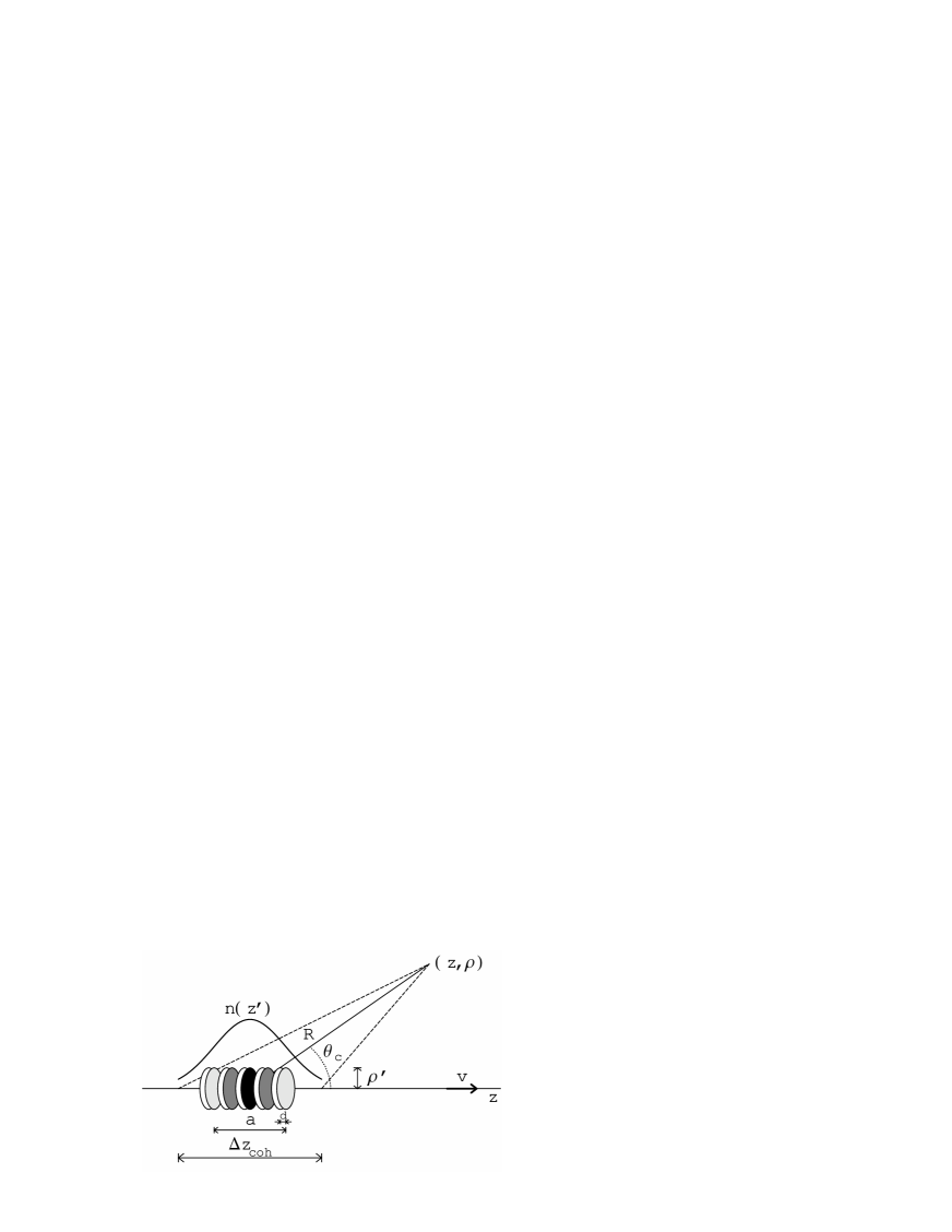
Consider (Figure 1) a charge moving on a straight line. Let $R(t)$ be the instantaneous distance from the charge to the observation point. Information propagating in the medium at speed $c_{m}$ will arrive simultaneously from the track if $\partial R/\partial t=c_{m}$. This is the Cherenkov condition: $\partial R/\partial t=v\cos{\theta}=c_{m}$ for velocity $\vec{v}$ oriented at angle $\theta$ relative to the direction $\hat{R}$. Note that $R(t)$ is the radius from the charge to the point, not the vector position.

Due to the geometry of the track and observation point, uniform motion produces acceleration of $R(t)$. If $\partial R/\partial t$ were constant, the fields arriving would all be in phase for the whole track length. However, the acceleration relative to the observation point produces an extra radial change of order $\Delta R=1/2(\partial^{2}R/\partial t^{2})(\Delta t)^{2}$. Coherence of modes of wavelength $\lambda$ is then maintained only over a finite region of $\Delta R<\lambda.$ Since $\partial^{2}R/\partial t^{2}=v^{2}\sin^{2}{\theta}/R$, we solve to find the condition $\Delta t_{coh}<\sqrt{R\lambda}/(v\sin{\theta})$. Equivalently, there is a finite spatial coherence region for given $R$, given wavenumber $k=2\pi/\lambda$, namely

$$\Delta z_{coh}<\sqrt{R/(k\sin^{2}{\theta})}$$

over which the “sonic boom” of radiation is built coherently. Since $\Delta z_{coh}\sim\sqrt{R}$, the coherence zone grows to infinite size as $R\rightarrow\infty$: but this limit cannot be taken carelessly.

2.3 Coherence of Evolving Charge Distributions

We now return to the emission from an electromagnetic shower or other time-evolving charge distribution. To a reasonable approximation, the number of particles in a highly relativistic shower scales like the primary energy divided by a suitable low energy threshold. The charge imbalance near the shower maximum is of order $20\%\,e$ of the total number of particles. These numbers have been confirmed over and over, with each generation of numerical simulation contributing further detail. The origin of the emitted Cherenkov power going like the shower-energy squared is basic electrodynamics: the electric field will scale like the charge, and the radiated power scales like the electric field-squared.

The evolving shower has a finite length scale $a$ over which it is near its maximum, and radiating copiously. This length scale, known as the “longitudinal spread” in cosmic ray physics [22], is akin to the length scale $L$ of Tamm’s approach but represents a smooth onset and decline of maximum power. The shower maximum-length scale $a$ is determined by the material, and is conceptually distinct from the shower’s total depth to reach the maximum (which goes like the logarithm of the energy) or the charged pancake size (which is fairly constant once the shower is developed.) A cartoon of these ideas is given in Figure 1.

There are then two characteristic limits. Suppose the longitudinal spread of the shower is “short” compared to the coherence length, $a\ll\Delta z_{coh}$. Then coherence is maintained over the whole range where the current is appreciable. The amplitude is proportional to the total length $a$ over which the current was “on”, times $1/R$. This is then the $R\rightarrow\infty$ limit, or Fraunhofer approximation, and looks like normal radiation. From dimensional analysis (and here we recall the discussion earlier), $E_{\omega}\sim a\omega/R$.

However, in the limit $a\geq\Delta z_{coh}$, the coherence length is not as big as the longitudinal spread, and coherence only exists over the smaller of the two. Adding amplitudes only over the region $\Delta z_{coh}$ and weighted by $1/R$, the $E_{\omega}$ field goes like $\omega\Delta z_{coh}/R=\sqrt{\omega/R}$. This behavior is rather different from the previous case: indeed Cherenkov radiation is fundamentally a Fresnel-zone effect, as seen by the $1/\sqrt{R}$ dependence of the fields.

Both the Fresnel and Fraunhofer limits are far-field approximations, in the sense that $kR\gg 1$ is assumed. The subtlety lies in the dimensionless ratio

$$\eta=(a/\Delta z_{coh})^{2}=\frac{ka^{2}}{R}\sin^{2}{\theta}$$

which controls how the limit $R\rightarrow\infty$ is taken. Confusion on this point is easy; one has $R/\lambda\sim 10^{4}$ in the same regime, and yet $R$ is not large enough for a “large $R$” Fraunhofer approximation to apply, exactly because the term “large R” is undefined until the limit parameter $\eta$ is specified. In the RICE experiment one typically has $a\sim 1-2m$, $\omega\sim 100-1000MHz$, and $R\sim 10^{3}m$, so $\eta<1$ holds. Extension to closer observation points, or to energies where the $LPM$ effect can give a much larger $a$, makes $\eta\gg 1$ possible. Partly due to the obscurity of the coherence criteria, the Fraunhofer approximation has received much attention in the previous literature [19, 18], except for those estimates using fields with ”cylindrical” symmetry [23, 17, 24, 25].

2.4 General Set-Up

Let $\vec{E}_{\omega}(x)$ be the time-Fourier transform of the $E$ field, with similar notation for other fields. The Maxwell equations for a dielectric medium are
$\vec{\nabla}\cdot\vec{D}_{\omega}=4\pi\rho,c\vec{\nabla}\times\vec{B}_{\omega}=4\pi\vec{J}_{\omega}-i\omega\vec{D}_{\omega},\vec{\nabla}\cdot\vec{B}_{\omega}=0,c\vec{\nabla}\times\vec{E}_{\omega}=i\omega\vec{B}_{\omega},$ where $\vec{D}_{\omega}(x)=\epsilon(\omega)\vec{E}_{\omega}(x)$. There is a wave equation for the vector potential $A^{\mu}_{\omega}(x)$, given by $c(\nabla^{2}+k^{2})A^{\mu}_{\omega}(x)=-4\pi J^{\mu}_{\omega}(x)$, with $k=\omega\sqrt{\epsilon}/c$. Then we have

$$c\vec{A}_{\omega}(\vec{x})=\int\!\!d^{3}\!x^{\prime}\,\frac{\exp{(ik|\vec{x}-\vec{x}\,^{\prime}|)}}{|\vec{x}-\vec{x}\,^{\prime}|}\int\!\!dt^{\prime}\,\exp{(i\omega t^{\prime})}\vec{J}(t^{\prime},\vec{x}\,^{\prime}).$$ (2)

The $4$-potential $A^{\mu}=(A^{0},\vec{A})$ has been defined in a generalized Lorentz gauge $c\vec{\nabla}\cdot\vec{A}+\epsilon\partial A^{0}/\partial t=0$ appropriate to the medium. The $4$-current $J^{\mu}=(\rho/{\epsilon},\vec{J})$, $\rho$. Since the components of $\vec{J}$ are related by $\vec{J}=\vec{v}\rho$, we have $\vec{A}=A^{0}{\epsilon}\vec{v}/c$. We calculate $\vec{A}_{\omega}$ and then use $A^{0}_{\omega}=\vec{v}\cdot\vec{A}c/(\epsilon v^{2})$. For radiation problems the denominator factor $1/|\vec{x}-\vec{x}\,^{\prime}|$ is replaced by $1/R$. This is standard, with corrections of order $a^{2}/R^{2}$ or similar effects in the “near field” regime, which is not our subject.

2.5 Evading The Fraunhofer Approximation

The Fraunhofer approximation is the textbook expansion for the phase
$\exp{(ik|\vec{x}-\vec{x}\,^{\prime}|)}\approx\exp{(ik|\vec{x}|-ik\hat{x}\cdot\vec{x}\,^{\prime})}$, dropping terms of order $k|\vec{x}\,^{\prime}|^{2}/R$. All existing simulations make this approximation for the phase, and for good reasons: the subsequent integrations become much simpler. The integrand in Eq. (2) oscillates wildly. A Monte Carlo simulation has to find the surviving phases from myriad cancellations, due to the phases generated over the length of each track, and then summed over thousands to millions of tracks moving in three dimensions. For a $1TeV$ shower the code of $ZHS$ runs in about 20 minutes on a workstation. Increasing the energy by a factor of 100, the calculational time scales up faster than linear, and computer time becomes prohibitive. For this reason various strategies to rescale the output have been used in arriving at the published values of electric fields. Even for $TeV$ energies, standard Monte Carlo routines such as GEANT challenge a work-station’s capacity. For cosmic rays of the highest energies the entire approach of direct numerical evaluation is unfeasible.

Unfortunately the Fraunhofer approximation also neglects terms in the phases, namely $k|\vec{x}\,^{\prime}|^{2}/R$, that may be of order unity given our previous discussion of length and frequency scales. We must avoid this step. Progress is possible due to the translational features of the macroscopic current
$J^{\mu}(t^{\prime},\vec{x}\,^{\prime})$. A rather general model is

$$\vec{J}(t^{\prime},\vec{x}\,^{\prime})=\vec{v}n(z^{\prime})f(z^{\prime}-vt^{\prime},\vec{\rho}\,^{\prime}).$$ (3)

An even more general situation will be discussed shortly. The charge packet travels with the speed $\vec{v}$, chosen here to be along the $z$-axis of the coordinate system. The function $f(z^{\prime}-vt^{\prime},\vec{\rho}\,^{\prime})$ represents a normalized charge density of the traveling packet, with $\vec{\rho}\,^{\prime}$ the transverse cylindrical coordinate relative to the velocity axis. We normalize $f$ by $\int\!\!dz^{\prime}d^{2}\!\rho^{\prime}\,f(z^{\prime},\vec{\rho}\,^{\prime})=1.$ In ice the packet is about $\Delta z^{\prime}=10cm$ thick in the longitudinal direction, and $\Delta\rho^{\prime}=10cm$ in radius (the Moliere radius) in the vicinity of the shower maximum. These size scales are limited because of relativistic propagation. The time evolution of these scales is negligible near the shower maximum, and indeed the Moliere radius is usually approximated by a material constant for the whole shower. Similarly, in air showers the scale of charge separation is small compared to the scale of shower longitudinal spread.

The shower’s net charge evolution appears in the factor $n(z^{\prime})$. With our normalization, $n(z^{\prime})$ represents the total charge crossing a plane at $z^{\prime}$. The symbol $n_{max}$ will denote the maxiumum value of $n(z^{\prime})$; later we will see that the electric field scales linearly with $n_{max}$. The longitudinal spread $a$ is a property of $n(z^{\prime})$ near the shower maximum. The model neglects charge (current) left behind, and moving at less than light-speed in the medium, which does not emit Cherenkov radiation. We do not have a sharp cut-off at the beginning or end of tracks, and the function $n(z^{\prime})$ will vary smoothly.

2.6 Factorization for the Fresnel Zone

Now while we cannot expand around $\vec{x}\,^{\prime}=0$ (the Fraunhofer approximation), the conditions of the problem do permit an expansion around $\vec{\rho}\,^{\prime}=0$ (the shower axis), namely for $R(z^{\prime})=[(z-z^{\prime})^{2}+\rho^{2}]^{1/2}$, that

$$|\vec{x}-\vec{x}\,^{\prime}| = [(z-z^{\prime})^{2}+(\vec{\rho}-\vec{\rho}\,^{\prime})^{2}]^{1/2},$$

$$= R(z^{\prime})-\frac{\vec{\rho}\cdot\vec{\rho}\,^{\prime}}{R}+{\cal O}(\frac{\rho^{\prime 2}}{R}).$$

For typical values in this problem, the second term is $\sim 10$ times smaller than the first, and the third is $\sim 10^{3}$ smaller than the second. For the exponent in Eq. (2), the third term does not contribute if $k\Delta\rho^{\prime 2}/R\ll 1$, that is $\omega\ll 250GHz$.

Collecting terms, we have

$$cR\vec{A}_{\omega}=\vec{v}\int dz^{\prime}\,n(z^{\prime})\exp{[i(\frac{\omega}{v}z^{\prime}+kR)]}$$

$$\times\int\int dt^{\prime}\,d^{2}\!\rho^{\prime}\,\exp{\{-i[\frac{\omega}{v}(z^{\prime}-vt^{\prime})+\vec{q}\cdot\vec{\rho}\,^{\prime}]}\}f(z^{\prime}-vt^{\prime},\vec{\rho}\,^{\prime}).$$ (4)

We have shifted the $t^{\prime}$ integral which produces the translational phase in the $z^{\prime}$ integral. This gives the factorization:

$$\vec{A}_{\omega}\approx F(\vec{q})\vec{A}^{FF}_{\omega}(\eta),$$ (5)

where

$$F(\vec{q})=\int\!\!d^{3}\!x^{\prime}\,e^{-i\vec{q}\cdot\vec{x}\,^{\prime}}f(\vec{x}\,^{\prime}),$$ (6)

$$vcR\vec{A}_{\omega}^{FF}=\vec{v}I^{FF},$$ (7)

and

$$I^{FF}(\eta,\theta)=\int\!\!dz^{\prime}\,\exp[\phi(z^{\prime})],$$

$$\phi(z^{\prime})=ik(z^{\prime}\cos{\theta_{c}}+R(z^{\prime},\rho))+\log{n(z^{\prime})}.$$ (8)

Here $\vec{q}=(\omega/v,\vec{q}_{\perp})$, $\vec{q}_{\perp}=k\vec{\rho}/R$, and $\vec{x}\,^{\prime}=(z^{\prime},\vec{\rho}\,^{\prime})$. Provided $F(\omega)\ll 1$ in either frequency region $k\Delta\rho^{\prime 2}/R\gg 1$ or $k\Delta z^{\prime 2}/R\gg 1$, the decoupling of the integrals is excellent. Here $\Delta\rho^{\prime}$ and $\Delta z^{\prime}$ refer to the regions over which the charge exists near the maximum. $F(\vec{q})$ is the form factor of the charge distribution, which happens to be defined, just as in the rest of physics, in terms of the Fourier transform of the snapshot of the distribution. From our definitions $F(0)=1$.

It is worth noting that the dependence on orientation of $\vec{q}$ is observable. For example, in a Giant Air Shower, where the mechanism of charge separation might cause an azimuthal asymmetry about the shower axis labeled by a dipole $\vec{p}$, then $F(\vec{q})$ depends on $F(\vec{q}\cdot\vec{p})$. The orientation of the dipole relative to the observation point thus has a strong effect on the emission. (Other numerically large effects will also be important: for example Allan[1] incorrectly assumes the fields go like $1/R$ from his use of Feynman’s formula).

As a consequence of separating out the form factor, the integrations have become effectively one-dimensional.

3 Numerical Work

At this stage we have a formula for the vector potential which is a product of a form factor and an object $I^{FF}(\eta,\theta)$ containing the information about the shower history. We will denote $I^{FF}(\eta,\theta)$ the Fresnel-Fraunhofer integral because it interpolates between these regimes. In the Fraunhofer approximation it is easily shown that the factorization is an exact kinematic feature of translational symmetry as exemplified in Eq. (3). If one makes a one-dimensional approximation, the Fraunhofer integral then evaluates the Fourier transform of the current[25, 26].

The factorization in the Fresnel zone is more demanding, yet should be an excellent approximation. When calculating $I^{FF}(\eta,\theta)$, we cannot (as mentioned earlier) consistently expand in powers of $z^{\prime}/R$ because $\eta\sim 1$ will be needed.

It makes sense at this point to make a numerical comparison with previous work. Summarizing the results of an extensive Monte Carlo calculation in the Fraunhofer approximation, $ZHS$ gave a numerical fit to the electric field

$$\frac{R|\vec{E}^{ZHS}_{\omega}(\theta)|}{F^{ZHS}(\nu)}=1.1\times 10^{-7}\frac{\nu}{\nu_{0}}\frac{E_{0}}{TeV}\exp{[-(\frac{\theta-\theta_{c}}{\Delta\theta})^{2}]}[\frac{V}{MHz}],$$ (9)

with $\nu_{0}=500MHz$. This is the result of a global fit to many angles, energies and frequencies $\nu=\omega/2\pi<\nu_{0}$. In this convention $\omega$ is positive. The normalized form factor is $F_{ZHS}(\nu)=1/[1+0.4(\nu/\nu_{0})^{2}]$, as discussed below. In making the calculation, results for the field were also rescaled due to computer limitations. As a result, the field reported is strictly linear in the primary energy $E_{0}$. We will comment on this shortly.

We calculated our own result proportional to $I^{FF}(\eta=0,\theta)$ over a range of many frequencies and angles (Figure 2). Before doing the integral we scale out the electromagnetic and dimensional factors which are obvious. In our convention $-\infty<\omega<\infty$. The results of our numerical integration are quite well fit by

$$\frac{R|\vec{E}^{\eta=0}_{\omega}(\theta)|}{F(\omega)}=\frac{e}{c^{2}}a\sqrt{2\pi}n_{max}\omega\sin{\theta}\exp{[-\frac{1}{2}(ka)^{2}(\cos{\theta}-\cos{\theta_{c}})^{2}]}$$ (10)

Putting in numerical values, this gives:

$$\frac{R|\vec{E}^{\eta=0}_{\omega}(\theta)|}{F(\omega)}=2.09\times 10^{-7}\frac{a}{m}\frac{n_{max}}{1000}\frac{\nu}{GHz}\exp{[-\frac{1}{2}(\frac{\cos{\theta}-\cos{\theta_{c}}}{\Delta(\cos{\theta})})^{2}]}[\frac{V}{MHz}],$$ (11)

where

$$\Delta(\cos{\theta})=0.048\frac{2}{\sqrt{\epsilon}}\frac{m}{a}\frac{GHz}{\nu}.$$

( We have indicated that $a$ is in units of $m.$ and $\nu$ in $GHz$.) Note the linear dependence on $a\nu$, argued earlier to come from dimensional analysis applied to the limit $\eta\rightarrow 0$. A cursory inspection shows that this result and the Monte Carlo have the same general features.

To continue the numerical comparison we need numbers for the longitudinal spread parameter $a$ and the number of charges at shower maximum $n_{max}$. There are several ways to estimate this. Running the $ZHS$ code many times and fitting the output of a $1TeV$ shower with a cutoff of $611KeV$ gives $a=1.5m$, $n_{max}=345$. Using these and allowing for the factor of two in conventions gives agreement to a few percent in normalization with $ZHS$. However, the other way to do the calculation is to evaluate the product $an_{max}$ many times. This method is preferred because fluctuations in $a$ and $n_{max}$ are correlated. Doing this gives $an_{max}=(570\pm 50)m$ at $1TeV$, which would predict a normalization factor of $(1.2\pm 0.1)\times 10^{-7}$ in Eq. (9). This (plus the angular dependence studied below) indicates that the factorized result is quite consistent with the Monte Carlo.

In Figure 2 we show numerically integrated values of $I^{FF}$ Eq. (8). These factors appear directly in the fit just cited, and serve to check the formulas. The form factor has been divided out. For the range of parameters relevant to the problem, agreement is very good, and relative error is much less than $1\%$.

For experimental purposes one would like independent confirmation of the parameters from another source. Net particle evolution is well described by Greissen’s classic solution, which was simplified further by Rossi to a Gaussian, $n(z)=n_{max}\,\exp{[-z^{2}/(2a^{2})]}/\sqrt{2\pi}a$. While Greissen’s $a$ refers to the whole shower, it should also be a reasonable description for the longitudinal spread of the charge imbalance, which tends to be a fixed fraction of the total number of particles after a few radiation lengths. (There is one caution that the Greissen formula does not explicitly include low-energy physics important for the charge imbalance.) The particular Greissen formula we consulted [27] for the longitudinal spread in radiation lengths $X_{0}$ gives $a/X_{0}\sim\sqrt{2/3log(E_{0}/E)}$ for particles in the shower with energy greater than $E$ and a primary with energy $E_{0}$. In that case one estimates $a=1.8m$ at $E_{0}=1TeV$ with $E=611MeV,X_{0}=0.39m$ in ice, which is acceptably close to the previous estimates.

At higher energies there is every reason to believe that Greissen’s
stretched $\sqrt{\log{E}}$ energy dependence will apply. In that case $a=2.1m$, $2.3m$ for $100TeV$, $1PeV$ showers, respectively. Note that the product $n_{max}a$ is relevant for the field normalization. In this case we also need $n_{max}\sim\\ 1/\sqrt{\log{(E_{0}/E)}-0.33}$ from the same Greissen approximation. Rather amazingly, the product $n_{max}a\sim(E_{0}/E)\sqrt{2/3\log{(E_{0}/E)}}/\sqrt{\log{(E_{0}/E)}-0.33}\\ \sim E_{0}/E$ at high energies. This confirms the phenomenon observed by $ZHS$: the normalization of the electric field (Fraunhofer approximation, $\theta=\theta_{c}$) scales precisely linearly in the primary energy. It is rather pleasing that the result can be understood from first principles [28]. Later we will see that the parameter $a$ enters in a much more complicated way in the Fresnel zone, creating an extra, weak energy dependence.

Regarding the angular dependence, our work (Figures 3) indicates a general dependence on $cos{\theta}-cos{\theta_{c}}$ rather than $\theta-\theta_{c}$. When fitting numerical output the two functional forms are rather different, unless one has a very narrow distribution. Linearizing for small $cos{\theta}-cos{\theta_{c}}$ with $a=1.5m$ for the comparison, we would predict the scale in the angular dependence $\Delta\theta=2.1^{o}(\nu_{0}/\nu)$ while $ZHS$ have the same expression with $2.4^{o}$. We find that $\Delta\theta$ is proportional to $1/a$. If $a$ grows slowly with energy, as Greissen’s formula indicates, then the angular width decreases, which is not seen in $ZHS$. Another possible explanation for the small discrepancy is the improper radiation from tracks terminating abruptly at the ends used in the Monte Carlo. We have identified these effects as responsible for the small oscillations seen in the Monte Carlo output, an effect apparently too small to measure.

When numerical output to the frequency dependence is fit, there is a slight coupling between the model for the form factor and the parameter $a$ one will extract for the longitudinal spread. We made our own fit to the $ZHS$ code’s frequency dependence including the region up to $1GHz$, using a Gaussian form factor because of its better analytic properties. (The $ZHS$ fit, which contains poles in both the upper and lower half-plane, violates causality.) Specifically, we find

$$F(\nu)=\exp{[-\nu^{2}/(2\nu_{*}^{2})]},\ \ \ \nu_{*}=0.93GHz.$$

Using the corresponding $a$ value we would predict the Fraunhofer Monte Carlo $\Delta\theta\sim 2.3^{o}(500MHz/\nu)$, quite close to $ZHS$.

In real life, shower to shower fluctuations are highly important. We studied the statistical features of the parameters $n_{max}$, $a$ by fitting individual showers many times and looking at the average and $rms$ fit values. The results at $E=1TeV$ were $a=1.5\pm 0.2m$, $n_{max}=345\pm 60$. Multiplying these and adding fluctuations in quadratures gives $an_{max}=520(1\pm 0.22)m$. The combination $an_{max}*$, which is the primary variable in determining the normalization of the electric field, was found to be $(570\pm 50)m$. The fluctuation of $an_{max}$ is less than half the value that the uncorrelated fluctuations of the separate terms would give. The relative fluctuation is said to decrease with increasing energy[28], but there are uncertainties. For example, threshold rescaling is used in Monte Carlos, leading to loss of information about the true fluctuations. Very preliminary results of running the standard Monte Carlo GEANT show variations in average shower parameters such as $an_{max}$ at the 30$\%$ level compared to the average of $ZHS$[31]. These comparisons indicate that the electrodynamics is probably determined better than the rest of the problem. Indeed, the deviations from Gaussian behavior in showers is an effect contributing to the fields at the few percent level. At the level of $10-15\%$, many other small effects contribute. Unless one uses details about the uncertainties and errors in fits, and especially about the shower-to shower fluctuations in all relevant quantities, it is pointless to fine-tune the comparison further. We conclude from the numerical work that the factorized expression is at least as reliable as the Monte Carlos, and has the attractive feature that the parameters can be adjusted directly.

4 The Saddle Point Approximation

While the Rossi-Greissen Gaussian approximation to the shower is common, there are additional features which favor such an approach to the emitted radiation. The coherence is dominated by regions where the phases add constructively, greatly enhancing the peak region. In such circumstances analysis is helpful, especially when the largest contribution to $I^{FF}$ is dominated by saddle points. These are points where the phase is stationary, $d\phi(z_{*})/dz_{*}=0$.

Here we describe the saddle-point method to evaluate $I^{FF}(\eta,\theta)$. This is a classic, controlled approximation when the charge distribution has a single maximum and $kR\gg 1$. The method turns out to give the exact result in the limit of flat charge evolution, that is, the Frank-Tamm formula, where numerical evaluation is highly unstable. With the saddle-point approximation, we can extract analytic formulas which are as good as the numerical integration.

We now describe the saddle-point features. By translational symmetry the shower maximum can be located at $z^{\prime}=0$. Referring to the formula of Eq. (8) cited earlier, the saddle point of the phase is given by solving

$$\cos{\theta_{c}}-(z-z_{*})/R(z_{*})-(i/k)(d/dz_{*})\log{n(z_{*})}=0$$

for the point $z_{*}$ dominating the integral. The maximum electric field is already known to occur at points $(z,R)$ near the Cherenkov cone. For such observation points $z=R\cos{\theta_{c}}$, and the saddle point equation has an easy solution at $z_{*}=0$. Thus the dominant integration region is near the shower maximum, as physically expected.

As the point of observation moves off the Cherenkov cone, the saddle point moves away into the complex $z^{\prime}$ plane. To find the complex saddle-point, we approximate $\log{n(z^{\prime})}\approx-z^{\prime 2}/(2a^{2})$ in the vicinity of the shower maximum; that is, we fit the top of the shower locally with a Gaussian. To re-iterate: the saddle-point approximation does not need to replace the entire shower by a Gaussian, but replaces the vicinity of the region where phases are contributing coherently by a Gaussian. The saddle-point condition gives a quartic equation which can be solved. Unfortunately the solution is impossibly complicated, thwarting a direct approach. We circumvented this by studying the saddle-point location numerically. We found the quartic solution is accurately linearized in a special variable: expand about $\cos{\theta}$ close to $\cos{\theta_{c}}$. We then find $z_{*}\approx R(0)\sin^{2}{\theta}(\cos{\theta}-\cos{\theta_{c}})[1+iR(0)/ka^{2}\sin^{2}{\theta}]^{-1}$. With this formula the reader inclined can repeat all the calculations. We also show the saddle-point to highlight the appearance of the ratio $R(0)/(ka^{2}\sin^{2}{\theta})$ indicated by the qualitative “acceleration” argument. Finally, replace $R(0)=R=\sqrt{z^{2}+\rho^{2}}$.

The rest of the calculation is standard mathematical physics [29], so we just quote the results. Calculating fields from the potential and keeping only the leading terms in $1/(kR)\ll 1$ we find:

$$\vec{E}_{\omega} = \frac{i\omega}{Rc^{2}}F(\vec{q})I^{FF}(\eta,\theta)[(\cos{\theta}-\cos{\theta_{c}})\vec{e}_{R}$$ (12)

$$-(1-i\eta\frac{\cos{\theta_{c}}}{sin^{2}{\theta}}\frac{\cos{\theta}-\cos{\theta_{c}}}{1-i\eta})\sin{\theta}\,\,\vec{e}_{\theta}],$$

$$\vec{B}_{\omega}=-\frac{i\omega}{vcR\cos{\theta_{c}}}F(\vec{q})I^{FF}(\eta,\theta)(1+i\eta\frac{\cos{\theta}}{sin^{2}{\theta}}\frac{\cos{\theta}-\cos{\theta_{c}}}{1-i\eta})\sin{\theta}\,\,\vec{e}_{\phi},$$ (13)

where

$$I^{FF}(\eta,\theta)=\!\!\!\!\!\! e^{ikR}a\sqrt{2\pi}[1-i\eta(\theta)(1-3i\eta\frac{\cos{\theta}}{\sin^{2}{\theta}}\frac{\cos{\theta}-\cos{\theta_{c}}}{1-i\eta})]^{-1/2}$$ (14)

$$\exp[-\frac{1}{2}(ka)^{2}\frac{(\cos{\theta}-\cos{\theta_{c}})^{2}}{1-i\eta}],$$

and where

$$\eta=\frac{ka^{2}}{R}\sin^{2}{\theta}.$$

Inspection reveals that these formulas have the dependence on $\omega$, $R$, and a distance scale $a$ quoted earlier on physical grounds. The formulas cited earlier as summarizing the numerical work are, in fact, the saddle-point approximations evaluated at $\eta=0$, which fit closer than any empirical formula.

4.1 Remarks

The dependence of the fields on symbol $\eta$ summarizes a good deal of complexity. For example:

• The limit $\eta\rightarrow 0$ yields the Fraunhofer limit, with spherical wave fronts and $E_{\omega}\sim a\omega/R.$

• The limit $\eta\rightarrow\infty$ gives the cylindrically symmetric $E_{\omega}\sim\sqrt{\omega/R}$ fields. This field can be substantially different from the Fraunhofer approximation. In fact one must take this limit to get the Frank-Tamm formula.

  A notable application is emission from ultra-high energy air showers. In such showers the $LPM$ effect plays a definite role in suppressing the soft emissions from the hardest charges. There is no corresponding suppression of the evolution of the low-energy regions of showers where most particles exist, however [30, 18]. The major effect that we find is that the showers become long kinematically: that is, the parameter $a$ gets big if one is working with, say, a primary of $10^{20}eV$. The emitted fields approach those of the Frank-Tamm formula as $a\rightarrow\infty$, via the formula cited. The effect is important numerically: a $10^{20}eV$ air shower does not approach the Fraunhofer limit nearer than $300km$. The conditions of RICE are more amenable to the limit, and at $R\sim 1km$, $\omega\sim 1GHz$ the Fraunhofer-based estimates near the Cherenkov cone in the literature are good to $20\%$.

• The frequency dependence in the Fraunhofer approximation is strongly affected by “diffraction”. Independent of the form factor effect, the Fraunhofer approximation imposes an upper limit to the frequency of order $\omega<(1/a)(\cos{\theta}-\cos{\theta_{c}})$. The true behavior is substantialli different: from Eq. (14) we see that the field exists in a region

  $$\omega<(1/a)[(\cos{\theta}-\cos{\theta_{c}})^{2}-(a^{2}/R^{2})\sin^{4}(\theta)]^{-1/2}.$$

  For large $\omega$ and in the angular region where the signal exists, the behaviour is much flatter. This is illustrated in Figures 4 and 5. This effect is invisible at the exact value $\theta=\theta_{c}$, where the fake Fraunhofer frequency cutoff and most of the true functional dependence in the exponent of $I^{FF}$ both drop out. As a result of the difference in frequency dependence, the time-structure of the electric field may be substantially different from the Fraunhofer approximation. We will return to this point in a Section Causal Features .

• Fields in the forward and backward directions, $\sin^{2}{\theta}\rightarrow 0$, are the fields of $\eta\rightarrow 0$, the Fraunhofer approximation, regardless of the physical values of $k,a,R$. We note that the experiments of Takahashi [13] observe an extremely limited region of $\sin^{2}{\theta}\rightarrow 0$. Perhaps this contributes to the observed agreement with Tamm’s formula in a regime where $a^{2}k/R$ is not close to zero.

• The polarization varies considerably. From symmetry the polarization is in the plane of the charge and the observation point. Moreover, for $\theta=\theta_{c}$ the electric field is transverse to $\vec{R}$ for any $\eta$. Yet naive transversality is not true in general at any finite $\eta$.

• Between the various limits the dependence on every scale in the problem, namely the frequency $\omega$, the distance $R$, the length scale $a$, and the angle $\theta$, is neither that of the Fraunhofer limit nor that of the infinite track Frank-Tamm limit, but instead a smooth interpolation between the cylindrical and spherical wave regimes.

• In the finite $\eta$ limit, one may also include a further effect, namely that as $\omega\rightarrow 0$ one has a ‘near-zone’ Coulomb-like response at small $R$. (Indeed, the $\omega\rightarrow 0$ limit measures the net charge.) This effect, important below about $10MHz$, also has a slight effect on the time structure of pulses.

We pause to comment on the generality of the result. What if we had not made the physical, but specific ansatz (3)? The entire analysis can be repeated for an arbitrary charge distribution $j(t^{\prime},z^{\prime},\vec{\rho}\,^{\prime})$. The Fraunhofer expansion of the transverse variable, and the Fourier integral of the $t^{\prime}$ variable are general. Provided the $\vec{\rho}\,^{\prime}$ extent is finite, and there exists a dominant $z^{\prime}$ region, then the integrals always factor into a product of a form factor and a one-dimensional integral for $A^{FF}_{\omega}(\eta)$. In fact nothing changes (the reader can repeat the calculation) except that when an arbitrary current is set up, the existence of a single saddle point cannot be assumed. Corrections to the local Gaussian approximation are straightforward. The slight skewness of real showers (or other arbitrary charge distributions) can also be developed as a saddle-point power series. Again: there are elements of bremmstrahlung in real showers, having a stochastic nature, which the current model has not attempted to reproduce. Detailed Monte Carlo simulations [31] of our group have included the bend-by-bend amplitudes of tracks undergoing collisions. This goes well beyond the approximation of a single straight line track, suddenly beginning and ending, of the previous literature [19, 18]. The effect of all the small kinks is negligible except in the very high frequency region $\omega\gg 100GHz$, while the endpoint accelerations give oscillations in the angular dependence down by orders of magnitude. As a final side remark: we explicitly studied contributions of finite tracks, just to see what would happen, in the development towards the conditions of the Tamm formula. It is straightforward to develop these pieces if one needs them for, say, the Takahashi-type experiments [13], in the Fresnel zone.

4.2 The General Case

We now turn to fields valid for any $\eta$. The form factor, which was extracted from the Fraunhofer calculations, is universal and need not be changed. The validity of the saddle-point approximation does not depend explicitly on the value of $\eta$. The procedure of linearization to locate the saddle-point happens to be good to $cos{\theta}-cos{\theta_{c}}\sim 1$, so that the approximation is rather good in the entire region $R/a\gg 1$, $kR\gg 1$.

For practical applications it is useful to have a formula for the fields with quantities measured in physically motivated units. For this purpose we rewrite (12) as follows

$$R\vec{E}_{\omega}\approx 2.52\cdot 10^{-7}\frac{a}{m}\frac{n_{max}}{1000}\frac{\nu}{GHz}F(\vec{q})\,\psi\,\vec{\cal{E}}\,\,[\frac{V}{MHz}].$$ (15)

Here $n_{max}$ is the excess of electrons over positrons at the shower maximum, $R$ is measured in meters, $\nu$ is measured in $GHz$. The rescaled field is

$$\vec{\cal{E}} = [-\frac{\cos{\theta}-\cos{\theta_{c}}}{\sin{\theta}}\vec{e}_{R}+(1-i\eta\frac{\cos{\theta_{c}}}{sin^{2}{\theta}}\frac{\cos{\theta}-\cos{\theta_{c}}}{1-i\eta})\,\,\vec{e}_{\theta}]$$ (16)

$$[1-i\eta(1-3i\eta\frac{\cos{\theta}}{\sin^{2}{\theta}}\frac{\cos{\theta}-\cos{\theta_{c}}}{1-i\eta})]^{-1/2}$$

$$\exp[-\frac{1}{2}(ka)^{2}\frac{(\cos{\theta}-\cos{\theta_{c}})^{2}}{1-i\eta}].$$

We have defined a kinematic factor $\psi=-i\exp(ikR)\sin{\theta}$ in such a way that the rescaled field $\vec{\cal{E}}$ is normalized at $\theta=\theta_{c}$,

$$\vec{\cal{E}}(\theta=\theta_{c})=(1-i\eta)^{-1/2}\,\,\vec{e}_{\theta}.$$ (17)

It is convenient to plot the magnitude of the rescaled field, Eq. (16). Figure 3 shows the magnitude as a function of the angle difference $\theta-\theta_{c}$ in various limits. The Fraunhofer approximation is shown by a dashed curve, and our result by the solid curve. One observes that the Fraunhofer limit is approached from below. This is physically clear: The Fresnel zone fields have a wider angular spread, and conservation of energy forces them to be smaller in magnitude compared to the sharper, diffraction-limited Fraunhofer fields. As the fields evolve to infinity, they coalese into narrower and taller beams.

The frequency dependence of $R|\vec{E}_{\omega}|/F(\omega)$ is shown on Figures 4 and 5. Exactly at the Cherenkov angle the difference between the Fraunhofer approximation and our results are minor for the typical parameters of $RICE$. However, away from the Cherenkov angle there is a substantial difference between the two, throughout the region where the magnitude of the field is large. This effect can be masked by the form factor, so we have plotted $RE_{\omega}/F(\omega)$ to show it. This effect may have important repurcussions for the time-structure of pulses, which are also discussed in the last Section.

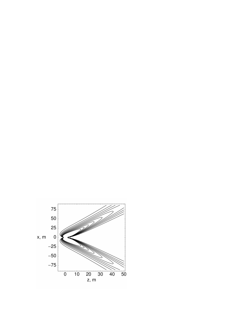
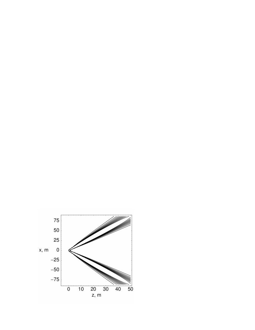
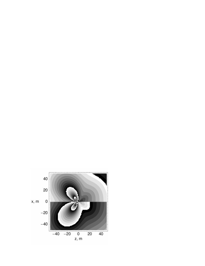
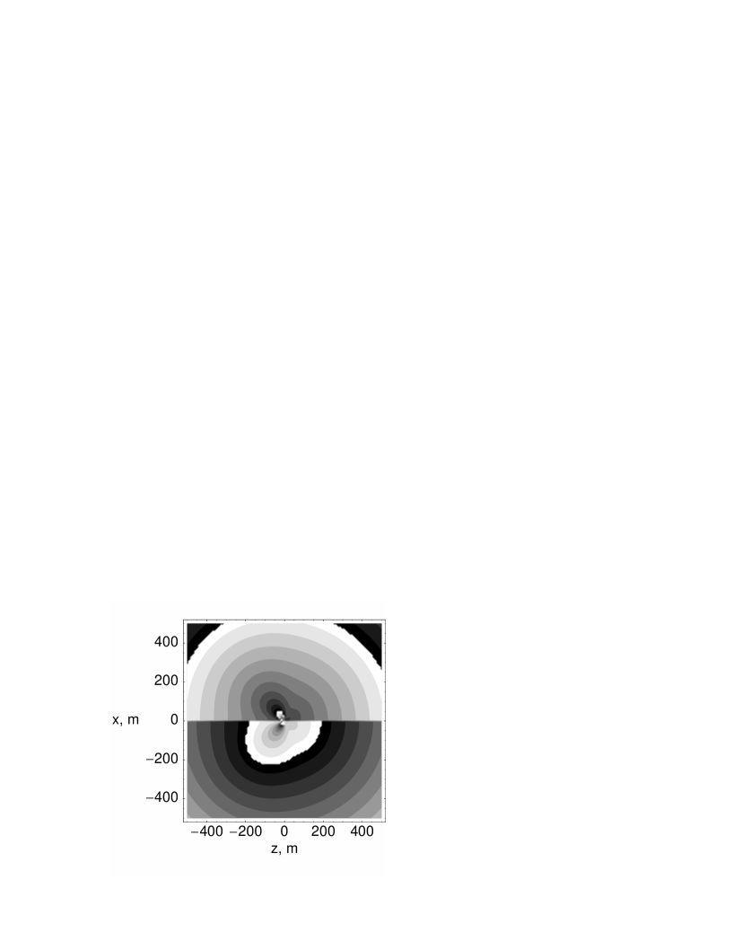
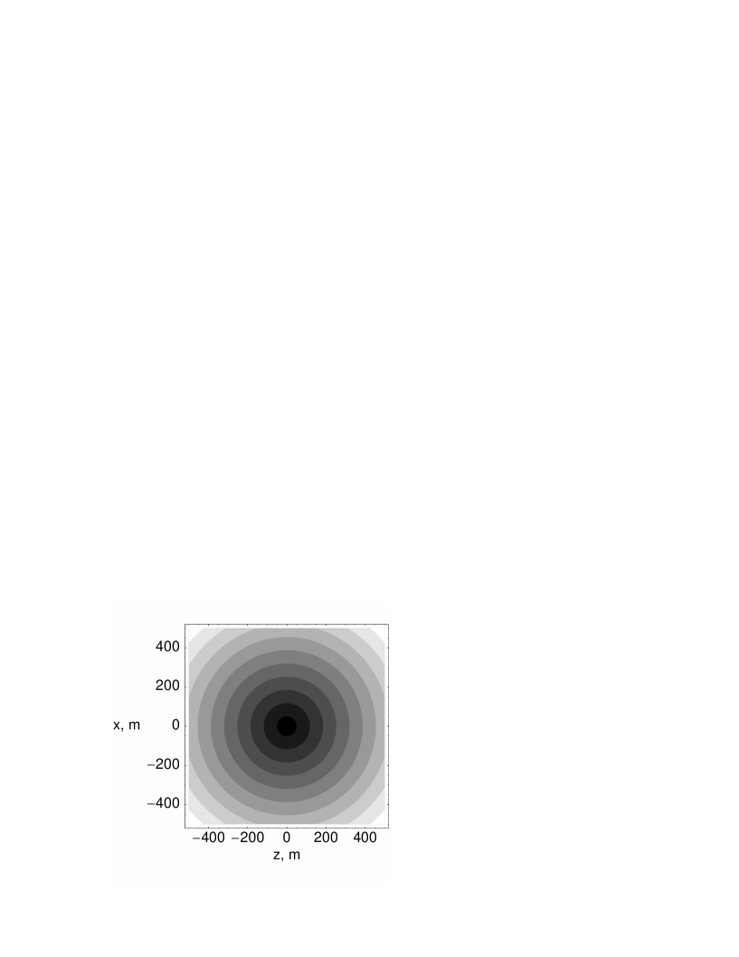
Figures 6-10 are contour plots of the electric field. We did not bother to remove the small region $a/R\sim 1$, where our result does not apply. The Fraunhofer approximation has trivial $1/R$ dependence on the distance to the observation point (Figure 10). The exact result is certainly different, with Figures 6, 8, and 9, in particular, illlustrating the effects of constructive interference in the region of cylindrical symmetry. A complementary view examines contour plots of constant phase. This is shown in Figures 8 and 9. In making these figures we decreased the kinematic phase $ikR$ to values showing several oscillations (as opposed to hundreds) across the range of the plots. The lines of constant phase can be used to illustrate the time-evolution of waves of a given frequency: that is, the Fourier transform of $\delta(\omega-\omega_{*})E_{\omega}exp(-i\omega t)$ has wave fronts at each moment in time given by the lines of constant phase. The constant phase lines of the Fraunhofer approximation are, of course, spherical (Figure 10). The constant phase lines of the true behaviour interpolate between cylindrical and spherical symmetry. As a consequence of the Fresnel-zone behaviour, the eikonals of the expanding radiation field do not emerge radially, but actually curve due to interference effects. This is a sobering impact of very basic physics, which has a measurable effect in the signal propagation speed discussed later under the topic of causal feature.

5 Causal Features

With our convention that the electric field $E(t,\vec{x})=1/(2\pi)\int_{-\infty}^{\infty}\!\!d\omega\,\exp(-i\omega t)\\ E_{\omega}(\vec{x})$, causality requires $E_{\omega}$ to be analytic in the upper half-plane of $\omega$. Singularities in the lower half-plane determine the details of $E(t,\vec{x})$ and the precise causal structure.

To discuss this we consider detection of signals via an antenna-system response function $\cal A_{\omega}$. By standard arguments the detected voltage is a convolution in time, and therefore a product in $\omega$ space, of the antenna function and the perturbing electric field. The antenna function has the same causal analytic properties as the electric field. A proto-typical antenna or circuit function for a driven $LRC$ circuit is

$${\cal A}_{\omega}=Z/(-\omega^{2}+\omega_{\cal A}^{2}-i\Gamma\omega),$$

where $Z$ depends on where the amplifier is connected in the circuit and can be treated as a constant. Note that $\cal A_{\omega}=-Z/(\omega-\omega_{+})(\omega-\omega_{-})$ where $\omega_{\pm}$ are in the lower half-plane. The dielectric function $\epsilon(\omega)$ can then be taken as slowly varying in the region where the antenna and form factor allow a response, and also has its analytic structure in the lower half-plane if this detail needs to be included. We will also ignore the form factor for this discussion, which earlier was cited as a formula analytic in the complex plane. While nothing in our analysis depends on these idealizations, this approach to the analytic structure serves to make our point.

As a first illustration, consider the electric field fit given by $ZHS$, proportional to $1/(\omega-i\omega_{0})(\omega+i\omega_{0})$ with $\omega_{0}/(2\pi)=500MHz$. This field has poles in both the upper and lower half-plane, violating causality. One may argue that the literal analytic behavior in the complex plane goes beyond the ambitions of the original semi-empirical fit. Nevertheless, Cauchy’s theorem applies to the subsequent numerical integrations that have been made [5], giving non-causal branches to numerically evaluated Fourier transforms, as well as unphysical short-time structure.

Let us compare the analytic structure of the electric field in the saddle-point approximation. This approximation does not attempt to describe the region $\omega\rightarrow 0$, which requires treatment of the near zone. However for causality we do not need $E_{\omega}$ near the origin but at large $|\omega|$. The saddle point approximation is good here so the results should be reliable.

Let us investigate this in more detail. In the exponent in the expression for the electric field we have $-(1/2)(ka)^{2}(\cos{\theta}-\cos{\theta_{c}})^{2}(1+i\eta)/(1+\eta^{2})$. Since $\eta$ goes like $\omega$ there is a phase linear in $\omega$ at large $|\omega|$. There is also a branch-cut and pole from the prefactor which occurs at $\eta=-i$. All singularities are in the lower half-plane and consistent with causality. The causal structure of $E(t,\vec{x})$ then hinges on closing the contour at infinity. For this the details of the antenna function, which generally has isolated singularities, as well as singular behavior of $E_{\omega}$ near the origin do not matter.

We close the contour at infinity avoiding the branch cuts, which may be oriented along the negative imaginary axis or as consistent. Convergence then requires

$$\lim_{\omega\rightarrow-i\infty}\mathrm{Re}[-i\omega t+i\omega\sqrt{\epsilon}R-\frac{1}{2}\omega^{2}\epsilon a^{2}(\cos{\theta}-\cos{\theta_{c}})^{2}\frac{i\eta}{1+\eta^{2}}]<0.$$

Using the definition of $\eta$, causality implies

$$t-\sqrt{\epsilon}\frac{R}{c}[1-\frac{(\cos{\theta}-\cos{\theta_{c}})^{2}}{2\sin^{2}{\theta}}]^{-1}>0.$$

This result has a natural interpretation. While the radiation from the shower appears to come primarily from the geometric location of the maximum, $\theta\sim\theta_{c}$, the shower actually develops and radiates earlier. Consequently the strict causal limit must correspond to an apparent propagation speed slightly faster than the naive speed of $c/\sqrt{\epsilon}$ deduced from the location of the observation point at $R$. The earliest signal actually arrives at an apparent speed $v_{app}$ of

$$v_{app}=\frac{c}{\sqrt{\epsilon}}[1-\frac{(cos{\theta}-cos{\theta_{c}})^{2}}{2\sin^{2}{\theta}}]^{-1}.$$

This formula is entirely geometrical, consistent with the simple picture that distance differences in the problem are causing the effect, but it also incorporates subtle features of coherence. For example, the distance scale $a$ cancels out. Yet $a$ determines the angular spread $\cos{\theta}-\cos{\theta_{c}}$ over which most of the power in the wave is contained, and enters in this fashion.

The Fraunhofer limit, in which all signals originate at a single point of origin, is incapable of capturing such an effect. It is interesting to trace the origin of the discrepancy. The singularities of interest are located by the zeroes of $1-i\eta=1-i\omega\sqrt{\epsilon}\sin^{2}{\theta}/R.$ When the limit $R\rightarrow\infty$ is taken in the first step of the Fraunhofer approximation, all the non-trivial analytic structure moves away to $\omega\rightarrow-i\infty$ and is lost. This procedure does not commute with closing the contour at $|\omega|\rightarrow\infty$. The correct procedure, of course, is to first close the contour, and then take the limit of large $R$.

In practice, of course, not all of the signal arrives at the earliest possible moment. The time scale over which the signal is detected depends on competition between dispersion, the antenna and form factor details, and something like twice the ”advanced” time interval. This time interval is $\Delta t_{caus}=R\sqrt{\epsilon}/(2c)(\cos{\theta}-\cos{\theta_{c}})^{2}/\sin^{2}{\theta}$. Since the $\Delta t_{caus}$ effect scales proportional to the distance $R$, it does not become negligible in any limit, exhibiting another subtle facet of breakdown of the Fraunhofer approximation.

Acknowledgments: This work was supported in part by the Department of Energy, the University of Kansas General Research Fund, the
K*STAR programs and the Kansas Institute for Theoretical and Computational Science. We thank Jaime Alvarez-Muñiz, Enrique Zas, Doug McKay, Soeb Razzaque and Suruj Seunarine for many helpful suggestions and conversations. We especially thank Enrique for writing and sharing the ZHS code, and Soeb and Suruj for generously sharing their results from running shower codes.

Figure 1: Cartoon of electromagnetic coherence zone associated with an evolving shower. The shower develops over a longitudinal spread dimension $a$, as represented by the smooth curve. During most of this development the pancake of charge has a constant size $d$, but an evolving charge normalization, represented by the gray scale. The coherence zone $\Delta z_{coh}$ depends on the angle, frequency, and location of the observation point. The situation illustrated has $\Delta z_{coh}>a$, a case in which full coherence of the charge (up to a frequency cutoff determined by the pancake size) is obtained. In the reverse limit $\Delta z_{coh}<a$, only the portion of the charge inside the region of $\Delta z_{coh}$ contributes constructively.

Figure 2: Comparison of numerically integrated (points) and analytic fit (solid curve) to the Fresnel-Fraunhofer integral $I^{FF}(\eta,\theta)$, Eq. (8). Values of parameters are: $a=1.5m$, $R=1000m$; frequency $\nu=1,2,5,10GHz$ (from top to bottom). Both Fresnel and Fraunhofer regimes are successfully reproduced. Angle is measured in degrees, $I^{FF}$ in meters.

Figure 3: Magnitude of the rescaled electric field $E=|\vec{{\cal E}}|$, Eq. (16). Our result (solid curve) is compared to the Fraunhofer approximation (dashed curve). $a=1.5m$, $R=50m$, $\nu=1GHz$; angle is measured in degrees. The Fraunhofer approximation is narrower in angular extent and larger in magnitude. Due to conservation of energy the field sharpens its angular distribution and approaches the asymptotically far field from below as $R\rightarrow\infty$. Up to scaling normalization factors, the same plot would apply to any with the same $\eta$, for example $a=3m$, $R=200m$.

Figure 4: Magnitude of the re-scaled electric field $W=(1000/n_{max})R|\vec{E}_{\omega}|/F(\omega)$ as a function of frequency $\nu$, evaluated at $\theta=\theta_{c}+1^{o}$. $W$ is measured in $10^{-7}V/MHz$. The dashed curve is the Fraunhofer approximation. Note the high frequency cutoff, which is not a form factor effect, but an artificial result of the limit $R\rightarrow\infty$ imposed by the approximation. Solid curve is our result. The parameters $a=1.5m$, $R=100m$.

Figure 5: Magnitude of the re-scaled electric field $W=(1000/n_{max})R|\vec{E}_{\omega}|/F(\omega)$ as a function of frequency $\nu$, evaluated at $\theta=\theta_{c}+0.3^{o}$. $W$ is measured in $10^{-7}V/MHz$. The dashed curve is the Fraunhofer approximation; solid curve our result. As $R\rightarrow\infty$ the Fraunhofer approximation begins to apply. The parameters $a=1.5m$, $R=1000m$.

Figure 6: Contour plot for the magnitude of the electric field. $a=5m$, $\nu=100MHz$, distances in $m$. Note the evolution of the field from cylindrical to spherical behaviour as the distance from the origin increases.

Figure 7: Contour plot for the magnitude of the electric field in the Fraunhofer approximation. The parameters $a=5m$, $\nu=100MHz$; distances in $m$. The magnitude of the field lacks the richness of structure of Figure 6.

Figure 8: Contour plot for the phase of the electric field. The parameters $a=1.5m$, $\nu=100MHz$; distances in $m$. Each contour represents the time evolution of an expanding wave front for the frequency used. The phases illustrate non-trivial propagation with destructive interference, as well as evolution from cylindrical to spherical symmetry.

Figure 9: Contour plot for the phase of the electric field. The parameters $a=1.5m$, $\nu=100MHz$; distances in $m$. The phases illustrate non-trivial propagation with destructive interference, here shown on a larger scale than Figure 8.

Figure 10: Contour plot for the phase of the electric field in the Fraunhofer approximation with $a=1.5m$, $\nu=100MHz$; distances in $m$. The contours illustrate kinematic spherical symmetry imposed by the approximation.

References

- [1] Allan, H. R., Progress in Elementary Particles and Cosmic Ray Physics, North-Holland Publishing Company, Amsterdam, 1971.
- [2] Askaryan, G. A., Zh. Eksp. Teor. Fiz. 41,616 (1961) [Soviet Physics JETP 14, 441 (1962)].
- [3] Jelly, J. V. et al, Nu. Cim. X46, 649 (1966)
- [4] Rosner, J. L. and Wilkerson, J. F., EFI-97-10 (1997), hep-ex/9702008; Rosner, J. L., DOE-ER-40561-221 (1995), hep-ex/9508011.
- [5] Frichter, G. M., Ralston J. P., and McKay, D. W., Phys. Rev. D 53, 1684 (1996).
- [6] Frichter, G., for the RICE collaboration, in 26th International Cosmic Ray Conference (Salt lake City 1999), edited by D. Kieda and B. L. Dingus (IUPAP 1999).
- [7] Provorov, A. L. and Zheleznykh, I. M., Astropart. Phys. 4 , 55 (1995).
- [8] Price, P. B., Astropart. Phys. 5, 43 (1996).
- [9] Andreev, Yu., Berezinsky, V., and Smirnov, A., Phys. Lett. B 84, 247 (1979); McKay, D. W. and Ralston, J. P., Phys. Lett. B 167 103 , 1986; Reno, M. H., and Quigg, C., Phys. Rev. D 37, 657 (1987); Frichter, G. M., McKay, D. W., and Ralston, J. P., Phys. Rev. Lett. 74, 1508-1511 (1995); Ralston, J. P., McKay, D. W., and Frichter, G. M., in International Workshop on Neutrino Telescopes, (Venice, Italy, 1996), edited by Baldo-Ceolin, M.; astro-ph/9606007; Gandhi, R., Quigg, C., Reno, M. H., Sarcevic, I., Phys. Rev. D 58 (1998) 093009.
- [10] Jain, P., McKay, D. W., Panda, S., and Ralston, J. P., hep-ph/0001031 (2000).
- [11] P. Jain, J. P. Ralston and G. Frichter, Astropart. Phys. 12, 193 (1999). See also J. P. Ralston, in 26th International Cosmic Ray Conference (Salt lake City 1999) edited by D. Kieda and B. L. Dingus (IUPAP 1999).
- [12] Gorham, P. W., Liewer, K. M., and Naudet, C. J.26th International Cosmic Ray Conference (Salt lake City 1999), edited by D. Kieda and B. L. Dingus (IUPAP 1999).
- [13] Takahashi, T., Kanai, T., Shibata, Y., et al., Phys. Rev. E 50, 4041 (1994).
- [14] Power, J. G., Conde, M. E., Gai, W., et al., ANL-HEP-CP-99-27, IEEE Particle Accelerator Conference (1999); Power, J. G., Gai, W., and Schoessow, P., ANL-HEP-PR-99-115, Phys. Rev. E 60, 6061 (1999); Cummings, M. A., Blazey J., Hedin, D., et al., FERMILAB-P-0896 (1996); Schoessow, P. and Gai, W., ANL-HEP-CP-98-35, 15th Advanced ICFA Beam Dynamics Workshop on Quantum Aspects of Beam Physics (1998).
- [15] Tamm, I. E., J. Phys. (Moscow) 1, 439 (1939).
- [16] Kahn, F. D. and Lerche, I., Proc. Roy. Soc. A 289, 206 (1966).
- [17] Ralston, J. P. and McKay, D. W., in Arkansas Gamma Ray and Neutrino Workshop: 1989, edited by Yodh, G. B., Wold, D. C., and Kropp, W. R., Nuc. Phys. B (Proc. Suppl) 14A 356 (1990); also reprinted in Proceedings of the Bartol Workshop on Cosmic Rays and Astrophysics at the South Pole (AIP, NY 1990) proceedings #198.
- [18] Alvarez-Muñiz, J., and Zas, E., Phys. Lett. B 411, 218 (1997).
- [19] Zas, E., Halzen, F., and Stanev, T., Phys. Rev. D 45, 362 (1992).
- [20] Perkins, D., Phil. Mag. 46, 1146 (1955).
- [21] Jain, P., Pire, B., and Ralston, J. P., Phys. Rep. 271, 67 (1996).
- [22] Rossi, B., High Energy Particles (Prentice Hall, New York, 1952).
- [23] Markov, M.A., and Zheleznykh, I. M., Mucl. Inst. Meth. Phys. Res. A248 , 242, (1986).
- [24] Jelley, J. V., Astroparticle Phys. 5, 255 (1996).
- [25] Jackson, J. D., Classical Electrodynamics, 2nd edition, John Wiley and Sons, Inc., New-York, 1975, p. 441ff.
- [26] Alvarez-Muñiz, J., Vázquez, R. A., and Zas, E., Phys. Rev. D 61, 023001 (1999).
- [27] T. K. Gaisser, Cosmic Rays and Particle Physics, (Cambridge University Press, 1990).
- [28] We thank Enrique Zas for discussion on these points.
- [29] Bender, C. M., and Orszag S. A., Advanced Mathematical Methods for Scientists and Engineers, McGraw-Hill Book Company, Inc., New-York, 1978.
- [30] Ralston, J. P. and McKay, D. W., in High Energy Gamma Ray Astronomy (Ann Arbor 1990), APS Conference Proceedings No. 220 (AIP, NY, 1991) J. Matthews, Ed.
- [31] Razzaque, S. et al., in preparation.