Impulsive and Varying Injection in GRB Afterglows

Abstract

The standard model of Gamma-Ray Bursts afterglows is based on synchrotron radiation from a blast wave produced when the relativistic ejecta encounters the surrounding medium. We reanalyze the refreshed shock scenario, in which slower material catches up with the decelerating ejecta and reenergizes it. This energization can be done either continuously or in discrete episodes. We show that such scenario has two important implications. First there is an additional component coming from the reverse shock that goes into the energizing ejecta. This persists for as long as the re-energization itself, which could extend for up to days or longer. We find that during this time the overall spectral peak is found at the characteristic frequency of the reverse shock. Second, if the injection is continuous, the dynamics will be different from that in constant energy evolution, and will cause a slower decline of the observed fluxes. A simple test of the continuously refreshed scenario is that it predicts a spectral maximum in the far IR or mm range after a few days.

1 Introduction

The standard model for GRB afterglows assumes that relativistic material is decelerating due to interaction with the surrounding medium. A shock wave is formed heating the surrounding matter to relativistic temperatures. It is assumed that both magnetic fields and accelerated electrons aqcuire an energy density which is a significant fraction of the equipartition value. In the simplest case, which will be referred to as the standard scenario, a single value of the energy and the bulk Lorentz factor is injected either as delta or as a top-hat function, of duration short respect to the afterglow. The total energy is fixed in time and equals the initial energy of the explosion.

Slower moving material is essential to all models which use density gradients as a means of acceleration. Actually, if this is indeed the mechanism, most of the system’s energy is carried by the slower material. This scenario overcomes the need for a clean environment. The fact that one now needs a substantially higher energy input can be addressed by a very energetic source such as a massive star. A similar situation exists in some cases of supernova. When a shock wave propagates through the envelope of the star arrives at the edge it accelerates, and higher and higher velocities are being imparted to a smaller fraction of the mass.

In GRB afterglows, if such slower material with significant energy is ejected, it will affect the evolution in two major ways: first, the system becomes more energetic as time passes (refreshed shock scenario), therefore the temporal decay of the afterglow will be slower (Rees & Mészáros 1998). Second, since the reverse shock will last for as long as the energy supply continues, it adds an additional long-living (reverse) emission component, typically at low frequencies. The emission from such a reverse shock was considered by Kumar & Piran (1999) for the discrete injection case. With accurate enough observations of the afterglow temporal decay or good spectral sampling, especially at radio to mm frequencies, both of these features may be detected, and could therefore constrain the possibility of additional energy injection.

2 Dynamics

We assume here that the source ejects a range of Lorentz factors. The simplest description is that there is a certain amount of mass $M(>\gamma)\propto\gamma^{-s}$ moving with a Lorentz factor greater than $\gamma$, all ejected at essentially the same time ( i.e., over a period which is much shorter than the afterglow timescales). The energy associated with that mass is $\gamma Mc^{2}\propto\gamma^{-s+1}$. Note that this is valid only for $s>1$ , were for $s<1$ the energy above any Lorentz factor is constant since it is all concentrated near the highest Lorentz factor. We normalize this proportionality using the initial Lorentz factor, $\gamma_{0}$, and the initial energy content, which is about the “burst” energy $E_{0}$:

$$E(>\gamma)\sim E_{0}(\gamma/\gamma_{0})^{-s+1},$$ (1)

down to some value $\gamma_{min}\leq\gamma_{o}$. This tilted top-hat injection leads to a “refreshed” shock scenario (Rees & Mészáros (1998)), in contrast to the standard straight top-hat or delta function model with a mono-energetic $E_{o}$ and a single value $\gamma_{o}$. Although $\gamma_{0}$ and $E_{0}$ are free parameters, we have lower limits on $\gamma_{0}\geq 100$ to avoid pair creation during the GRB itself, and we have an estimate of the initial energy $E_{0}$ from the energy seen in the burst. The actual value of $\gamma_{0}$ can be obtained from the onset time of the afterglow or from the reverse shock initial frequency. This scenario is related to, but not identical, to the Fenimore & Ramirez-Ruiz (1999) model in which a wind with near-steady $\gamma$ impacts on a decelerating ’wall’ produced by the outermost shells of material which first make contact with the exterior gas. The refreshed shock or tilted top-hat scenario envisages an ’engine’ duration which is instantaneous compared to the deceleration time, whereas the latter scenario assumes that the wind duration is longer than the initial deceleration time. However if the ’engine’ produced a wind whose Lorentz factor decreased with time, the net effect could be rather similar to the refreshed shock.

The low Lorentz factor mass will catch up with the high Lorentz factor mass only when the latter has decelerated to a comparable Lorentz factor. At that time the shocked material (both reverse and forward shock) has a Lorentz factor $\gamma$ satisfying

$$E_{0}(\gamma/\gamma_{0})^{-s+1}\sim E\sim\gamma^{2}R^{3}\rho c^{2}.$$ (2)

If we assume that the outer density is $\rho\propto R^{-g}$, then we have

$$\gamma=\gamma_{0}(R/R_{0})^{-(3-g)/(1+s)}$$ (3)

Using the relation $t\sim R/\gamma^{2}c$ we get

$$R = R_{0}(t/t_{0})^{(1+s)/(7+s-2g)}$$ (4)

$$\gamma = \gamma_{0}(t/t_{0})^{-(3-g)/(7+s-2g)}~{},$$

where $R_{0}$ and $t_{0}$ are the deceleration radius and deceleration time of the initial material with $E_{0},~{}\gamma_{O}$. Note that these scalings differ from those of Rees and Mészáros (1998), who obtained $s+1$ where we have $s$ in the scalings of expressions after our equation (2). For $s=1$ the energy in the slow material adds up only logarithmically and therefore the above expression degenerates to the usual ones of instantaneous injection. However, for $s>1$ where more energy is stored in a slowly moving material, we have a slower decay as more and more energy is added to the system as time evolves. Note also that these expression are only valid for $g<3$. Otherwise, the shocks is accelerating (see Blandford & Mckee for $3<g<4$ and Best & Sari for $g>4$). However, the most useful values of $g$ are probably the constant density case $g=0$ and the wind case $g=2$.

Since the additional slow shells catch up with the shocked material once these are with comparable Lorentz factors, the reverse shock is always mildly relativistic (Rees & Mészáros 1998, Kumar and Piran 1999). The thermal Lorentz factor of the electrons is therefore roughly given by the ratio of proton to electron mass $\gamma_{e}^{r}\sim\epsilon_{e}m_{p}/m_{e}$. In the forward shock, the thermal Lorentz factor of the electrons is $\gamma_{e}^{f}\sim\epsilon_{e}\gamma m_{p}/m_{e}$.

The pressure behind the reverse shock is proportional to the density behind the reverse shock which is comparable to the density in front of it (a mildly relativistic shock) therefore

$$p_{r}\propto n_{r}\propto\frac{M}{R^{3}/\gamma}\propto t^{-\frac{6+sg-g}{7+s-2g}}.$$

As a check we can see that this is also the pressure at the forward shock which is proportional to $\gamma^{2}\rho$. The forward and reverse shock have the same bulk Lorentz factor and the same pressure, while the forward shock has a temperature which is higher by a factor of $\gamma$.

3 Radiation

The dynamics above determine the bulk Lorentz factor and the thermal Lorentz factor of the electrons as function of time. To estimate the resulting synchrotron radiation, one also needs an estimate of the magnetic field. For a given magnetic field, the spectrum consists of four power law segments separated by three break frequencies $\nu_{a}$, $\nu_{m}$ and $\nu_{c}$ (Sari, Piran and Narayan 1998, Mészáros , Rees & Wijers 1998). Adopting the standard assumption that the magnetic energy density is some fraction $\epsilon_{B}$ of equipartition, i.e., proportional to the pressure, we have

$$B\propto t^{-\frac{1}{2}\frac{6+sg-g}{7+s-2g}}.$$

Since the pressure in the reverse and forward shock is identical, the magnetic field will also be the same, if the equipartition parameter $\epsilon_{B}$ is the same. The difference between the forward and reverse shock lies then in the number of electrons (which is larger by a factor of $\gamma$ at the reverse shock) and their thermal Lorentz factor (which is smaller by a factor of $\gamma$ at the reverse shock). This result in the following general properties, valid at any given moment:

1) The peak flux of the reverse shock, at any time, is larger by a factor of $\gamma$ than that of the forward shock: $F_{\nu,\max}^{r}=\gamma F_{\nu,\max}^{f}$

2) The typical frequency of the minimal electron in the reverse shock is smaller by a factor of $\gamma^{2}$: $\nu_{m}^{r}=\nu_{m}^{f}/\gamma^{2}$.

3) The cooling frequency of the reverse and forward shock are equal: $\nu_{c}^{r}=\nu_{c}^{f}=\nu_{c}$.

4) At sufficiently early time (typically the first few weeks or months) $\nu_{a}^{r,f}<\nu_{m}^{r,f}$ and $\nu_{a}^{r,f}<\nu_{c}$. The sefl absorption frequency of the reverse shock is larger than that of the forward shock. It is larger by a factor of $\gamma^{3/5}$ initially, when both are in fast cooling and by a factor of $\gamma^{8/5}$ if both are in slow cooling.

Points one and two above agree with those of Kumar and Piran, calculated for the discrete case. We have here generalized the result to include the effect of the cooling frequency and self absorption frequency. The combined reverse+forward shock emission can therefore be one of three types, evolving in time in the following order:

A) Both reverse and forward shock are cooling fast: $\nu_{a}^{f}<\nu_{a}^{r}<\nu_{c}<\nu_{m}^{r}<\nu_{m}^{f}$.

B) Reverse is slow cooling, forward is fast cooling: $\nu_{a}^{f}<\nu_{a}^{r}<\nu_{m}^{r}<\nu_{c}<\nu_{m}^{f}$.

C) Both reverse and forward shock are in slow cooling, $\nu_{a}^{f}<\nu_{a}^{r}<\nu_{m}^{r}<\nu_{m}^{f}<\nu_{c}$.

These three spectra are presented in figure 1. As evident from the figure, the forward shock dominates the emission at very low and very high frequencies while the reverse shock contributes to a spectral “bump” at intermediate frequencies. The peak flux is that of the reverse rather than the forward shock. The combined spectrum is somehwat flatter than the usual one (which uses the forward shock only). A good sampling of the spectrum, especially at low frequencies, can therefore show the existence or non-existence of such a feature. The forward shock alway dominates above $\nu>\max(\nu_{m}^{f},\nu_{c})$ by a small factor of $\gamma^{p-2}$. Since the value of $p$ is close to $2$, the forward shock does not radiate much more than the reverse at high frequencies.

– FIGURE 1 –

In the case of fast cooling we have ignored the effect of the ordered structure of the electron’s energy behind the shock (Granot, Piran & Sari (2000)), both for the reverse and forward shock. This effect will increase the emission at frequencies below the self absoption frequency, $\nu<\nu_{a}$, but will not change the qualitative conclusions of this paper.

The spectrum displayed in figure 1 is valid at any moment if the energy and momentum injection is continuous, but also at the moment of impact in the case of the standard top-hat injection. However, in the latter case the reverse shock component will rapidly disappear as discussed by Sari & Piran 1999 and Mészáros & Rees 1999. If the injection is discrete, the dynamics of the forward shock right after the collision will not be affected, and it will evolve as in the standard non-refreshed scenario. .

For the continuous case, the time dependence $t^{-q}$ of the various quantities is given in Table 1, for arbitrary parameters $s$ and $g$, assuming a spectral shape $\propto\nu^{-\beta}$. Above the peak $\nu_{max}=\min[\nu_{m},\nu_{c}]$ where the flux has the value $F_{\nu,max}$ the dependence $F_{\nu}\propto t^{-\alpha}\nu^{-\beta}$ is calculated separately for the slow and fast cooling regimes.

– TABLE 1 –

To give more specific numerical examples we specialize to the constant density case, where $g=0$. We then have

$$\nu_{m}^{f}=2.0\times 10^{13}{\rm Hz\,}(1+z)^{1/2}\epsilon_{B,-2}^{1/2}\epsilon_{e,0.5}^{2}E_{52}^{1/2}t_{day}^{-3/2}(\frac{t}{t_{0}})^{\frac{3(s-1)}{2(7+s)}}$$ (5)

$$\nu_{m}^{r}=9.1\times 10^{11}{\rm Hz\,}(1+z)^{-1/4}\epsilon_{B,-2}^{1/2}\epsilon_{e,0.5}^{2}E_{52}^{1/4}n_{0}^{1/4}t_{day}^{-3/4}(\frac{t}{t_{0}})^{\frac{3(s-1)}{4(7+s)}}$$ (6)

$$\nu_{c}=2.7\times 10^{15}{\rm Hz\,}(1+z)^{-1/2}\epsilon_{B,-2}^{-3/2}E_{52}^{-1/2}n_{0}^{-1}t_{day}^{-1/2}(\frac{t}{t_{0}})^{-\frac{3(s-1)}{2(7+s)}}$$ (7)

$$F_{\nu,max}^{f}=2.6{\rm mJy\,}(1+z)\epsilon_{B,-2}^{1/2}E_{52}n_{0}^{1/2}D_{L,28}^{-2}(\frac{t}{t_{0}})^{\frac{3(s-1)}{7+s}}$$ (8)

$$F_{\nu,max}^{r}=12{\rm mJy\,}(1+z)^{11/8}\epsilon_{B,-2}^{1/2}E_{52}^{9/8}n_{0}^{3/8}D_{L,28}^{-2}t_{day}^{-3/8}(\frac{t}{t_{0}})^{\frac{27(s-1)}{8(7+s)}}$$ (9)

For slow cooling, $\nu_{c}>\nu_{m}>\nu_{a}$, the spectral peak is at $\nu_{max}=\nu_{m}$, and synchrotron self-absorption occurs at

$$\nu_{a}^{f}=3.6{\rm GHz\,}(1+z)^{-1}\epsilon_{e,0.5}^{-1}\epsilon_{B,-2}^{1/5}E_{52}^{1/5}n_{0}^{3/5}(\frac{t}{t_{0}})^{\frac{3}{5}\frac{s-1}{7+s}}$$ (10)

$$\nu_{a}^{r}=43{\rm GHz\,}(1+z)^{-2/5}\epsilon_{e,0.5}^{-1}\epsilon_{B,-2}^{1/5}E_{52}^{2/5}n_{0}^{2/5}t_{day}^{-3/5}(\frac{t}{t_{0}})^{\frac{6(s-1)}{5(7+s)}}$$ (11)

while for fast cooling, $\nu_{m}>\nu_{c}>\nu_{sa}$, the spectral peak is at $\nu_{max}=\nu_{c}$ and we have

$$\nu_{a}^{f}=0.3{\rm GHz\,}(1+z)^{-1/2}\epsilon_{B,-2}^{6/5}E_{52}^{7/10}n_{0}^{11/10}t_{day}^{-1/2}(\frac{t}{t_{0}})^{\frac{21}{10}\frac{s-1}{7+s}}$$ (12)

$$\nu_{a}^{r}=0.8{\rm GHz\,}(1+z)^{-11/40}\epsilon_{B,-2}^{6/5}E_{52}^{31/40}n_{0}^{41/40}t_{day}^{-29/40}(\frac{t}{t_{0}})^{\frac{93(s-1)}{40(7+s)}}$$ (13)

Using the normalization of the peak flux and the break points, the flux can be calculated at any frequency. Similar to the standard case, it is possible to test the model by comparing the temporal decay and spectral slopes.

In the standard case (mono-energetic instantaneous injection), the flux above this frequency is falling with time, while the flux below this frequency is rising with time. The additional energy in the varying injection case tends to flatten the decay rate, and for high enough values of $s$ can even make it grow. (From equations (1) and (4) one sees that the $t/t_{0}$ factors in equations (5)-(13) are equivalent to a power of the ratio of the injected to initial energy $E/E_{0}$). Stated differently, one would need a steeper spectral index to give rise to the same observed temporal decay in the refreshed scenario. Table 2 summarizes for $g=0$ the values of the spectral index $\beta$ that can be inffered from a measured temporal decay index $\alpha$ in the instantenous and refreshed scenarios, for reverse and forward shocks.

– TABLE 2 –

It can be seen that the spectal indices that need to exmplain a $t^{-1}$ decay that is observed in many bursts are considerably steeper. Some confusion can occur between a forward moderately refreshed ($s=2$) shock in the slow cooling regime and a fast cooling forward shock in the non-refreshed scenario, as these two scenarios predict similar relation between $\alpha$ and $\beta$ for nominal values. However, most other regimes are considerably different from the standard instanteneous forward shock prediction even if one only has moderately accurate spectral data information.

4 Specific Bursts

GRB 970508. - In the case of GRB 970508, the observations show a steep increase in the optical and X-ray fluxes between one and two days. This can be interpreted in terms of a varying injection event, e.g. Panaitescu, Mészáros & Rees 1998, who consider the radiation of the forward shock assuming a large value of $s$, a value of $\gamma_{min}=11<\gamma<\gamma_{o}$ and a final energy $E_{f}=3E_{o}$. After this time the energy is constant, and the afterglow can be fitted with a standard mono-energetic afterglow, e.g. Wijers & Galama 1999. How could we test the hypothesis that the ”jump” between half a day to two days is indeed due to varying injection? It turns out that a delayed energy injection (if $\epsilon_{B}$ is the same for the reverse and forward shocks) has a very strong prediction. We can estimate the forward shock break frequencies at $t=2$ days by extrapolating them back from those at day 12, where the spectrum is well studied (e.g. Wijers & Galama (1999), Granot, Piran & Sari 1999b ). This results in $\nu_{m}^{f}\cong 1.3\times 10^{12}$ Hz, $F_{\nu,max}\sim 1.7$mJy, $\nu_{a}^{f}\cong 3$ GHz and $\gamma=4$. Therefore, according to the lower frame of figure 1 the reverse shock should have $\nu_{m}^{r}\cong 80$GHz and $\nu_{a}^{r}\cong 30$GHz. The reverse shock signature should be the largest between these two frequencies, where the flux should exceed by an order of magnitude the simple extrapolation of the forward shock model back to day two. At a more observationally accessible frequency of $20$GHz and $100$GHz the flux increase due to the reverse shock should be a factor $\sim 5$ and $\sim 8$ respectively, i.e. a flux of $2.2$mJy and $6$mJy, respectively. Unfortunately, the observations around 2 days at these frequencies where short and therefore of low sensitivity. The $3\sigma$ upper limit of $6$mJy obtained by BIMA is consistent with energy injection. This prediction of an additional low frequency component in GRB 970508 is similar to that of Kumar & Piran (1999). However, taking the self absorption frequency into account we have shown here that this would not apply to the usually observed radio frequencies $1.4$GHz-$8.4$GHz but to the range of $30$GHz-$80$GHz. It is therefore of great value to obtain low frequency observations or strong upper limits if such jumps in the optical and X-ray flux will be seen again in the future. If the reverse shock signature is not seen in other comparable bursts where a light curve peak is detected at a certain time (1.5 days in this case), a varying injection episode can be ruled out as an explanation for this peak (or else, it would imply $\epsilon_{B,rev}\ll\epsilon_{B,for}$).

GRB 990123. - In GRB 990123, a bright 9th magnitude prompt flash was seen about 60s after the trigger time (Akerlof, et al. (1999)), attributable to a reverse shock (Sari & Piran 1999a ; Mészáros & Rees (1999) with an initial temporal decay $F\propto t^{-2}$, steeper than the subsequent decay $F\propto t^{-1.1}$ which is attributable to the forward shock. Here, an impulsive mono-energetic (standard) injection fits better than a tilted top-hat, since e.g a varying $s=2,g=0$ injection would predict a decay $\alpha=1$, while an impulsive event gives $\alpha=2$, in good agreement with observations for a spectral slope $\beta=1$ in the fast cooling regime (the values are 2/3 and 9/8 in the adiabatic regime). Though no spectral information was available for this burst in the first hours, a slope $\beta\leq 1$ can be assumed based on our accumulated knowledge from previous afterglows.

5 Discussion

The dynamics and emission of the forward and reverse shocks is controlled by several factors, including the continuity and nature of the energy and mass input, the possible existence of external density gradients, and the strength of the magnetic fields in these regions. A contineous injection of energy with a lower Lorentz factor has as its main consequence that it tends to flatten the decay slopes of the afterglow, after it has gone through the maximum. An external density gradient (e.g. as in a wind with $\rho_{ext}\propto r^{-g}$, where $g\sim 2$ might be typical) has the property of steepening the decay. This applies in general both to the forward and the reverse shocks.

We have suggested ways in which one can attempt to discriminate between the standard straight top-hat injection of energy and momentum with a single $\gamma_{o}$ and $E_{o}$, which then remains constant throughout the afterglow phase, and a refreshed scenario, where the injection is also brief (e.g. comparable to the gamma-ray burst duration and therefore instantaneous compared to the afterglow timescale) but in which there is a varying distribution of $\gamma$ and of energy during that injection, so that matter ejected with low Lorentz factor cateches up with the bulk of the flow on long timescales. The afterglow energy then increases with time. Under the simple assumption that both the forward and the reverse magnetic fields are equal ($\epsilon_{B,r}=\epsilon_{B,f}$) a remarkable prediction is that in all regimes (both shocks are fast cooling, reverse is slow cooling and forward shock is fast cooling or both are slow cooling) the reverse shock spectrum joins seamlessly, or with only a very modest step $\propto\gamma^{p-2}$, onto the forward shock spectrum, extending it to lower frequencies. (This could be modified if, for instance, $\epsilon_{Br}\ll\epsilon_{Bf}$, which would give a spectrum with a more pronounce through separating the reverse and forward components). Specifically, in the case of GRB 970508, if a descrete episode of injection that produced refreshed shocks at $t\sim 1.5$ days is the explanation of the step in the X-ray and optical flux at this time, then one would expect (for equal forward and reverse $\epsilon_{B}$) an even more dramatic rise of the 20 GHz and 100GHz flux at 1.5-2 days. This should be about a factor of 5 and 8, respectively, larger than expected from the forward shock values extrapolated back to 2 days. In the case of GRB 990123 a reverse shock appears to have been responsible for the prompt optical flash, and the decay indices (for reasonable spectral slopes) are compatible with monoenergetic impulsive (or straight top-hat) injection.

For future GRB afterglow observations, the main prediction from having comparable values of $\epsilon_{B}$ in the forward and reverse shocks of baryon loaded fireballs is that the peak flux is found at the peak frequency of the reverse, rather than of the forward shock, i.e. at lower frequencies than typically considered. The IR, mm and radio fluxes would therefore be expected to be significantly larger than for simple (forward shock) standard afterglow models (e.g. Fig 1). This holds whether the injection in contineous or descrete. The two contributions continue to evolve as a pair of smoothly joined components, the ratio of the two peak frequencies $\nu_{m}^{r}/\nu_{m}^{f}\propto\gamma^{-2}$ and peak fluxes $F_{\nu,mr}/F_{\nu,mf}\propto\gamma$ gradually approaching each other until they coincide at the transition to the non-relativistic case $\gamma\sim 1$.

	$\nu_{m}$	$F_{\nu_{m}}$	$\nu_{c}$	$F_{\nu}$: $\nu_{m}<\nu<\nu_{c}$	$F_{\nu}$: $\nu>\max(\nu_{c},\nu_{m})$
f	-$\frac{24-7g+sg}{2(7+s-2g)}$	$\frac{6s-6+g-3sg}{2(7+s-2g)}$	-$\frac{4+4s-3g-3sg}{2(7+s-2g)}$	-$\frac{6-6s-g+3sg+\beta(24-7g+sg)}{2(7+s-2g)}$	-$\frac{-4-4s+g+sg+\beta(24-7g+sg)}{2(7+s-2g)}$
r	-$\frac{12-3g+sg}{2(7+s-2g)}$	$\frac{6s-12+3g-3sg}{2(7+s-2g)}$	-$\frac{4+4s-3g-3sg}{2(7+s-2g)}$	-$\frac{12-6s-3g+3sg+\beta(12-3g+sg)}{2(7+s-2g)}$	-$\frac{8-4s-3g+sg+\beta(12-3g+sg)}{2(7+s-2g)}$

Table 1: Temporal exponents of the peak frequency $\nu_{m}$, the maximum flux $F_{\nu_{m}}$, the cooling frequency $\nu_{c}$ and the flux in a given bandwidth $F_{\nu}$, calculated both in the adiabatic regime $\nu_{m}<\nu<\nu_{c}$ ($F_{\nu}\propto F_{\nu_{m}}(\nu_{m}/\nu)^{\beta}\propto t^{-\alpha}\nu^{-\beta}$, where $\beta=(p-1)/2$), and in the cooling regime $\nu_{c}<\nu_{m}<\nu$ ($F_{\nu}\propto(\nu_{c}/\nu_{m})^{1/2}(\nu_{m}/\nu)^{\beta}\propto t^{-\alpha}\nu^{-\beta}$ where $\beta=p/2$).

		spectral index $\beta$, as function of $\alpha$ ($F_{\nu}\propto t^{-\alpha}\nu^{-\beta}$)
Shock	Regime	no-injection		$s=2$		$s=3$
forward	$\nu_{m}<\nu<\nu_{c}$	$\frac{2\alpha}{3}$	$\left[2/3\right]$	$\frac{3\alpha+1}{4}$	$\left[1\right]$	$\frac{5\alpha+3}{6}$	$\left[4/3\right]$
forward	$\nu>\max({\nu_{m},\nu_{c}})$	$\frac{2\alpha+1}{3}$	$\left[1\right]$	$\frac{3\alpha+2}{4}$	$\left[5/4\right]$	$\frac{5\alpha+4}{6}$	$\left[3/2\right]$
reverse	$\nu_{m}<\nu<\nu_{c}$	short-lived		$\frac{3\alpha}{2}$	$\left[3/2\right]$	$\frac{10\alpha+3}{6}$	$\left[13/6\right]$
reverse	$\nu>\max({\nu_{m},\nu_{c}})$	short-lived		$\frac{3\alpha}{2}$	$\left[3/2\right]$	$\frac{5\alpha+1}{3}$	$\left[2\right]$

Table 2: The spectral indices $\beta$ that would be deduced from an observed temporal decay index $\alpha$. The third column gives the well known “standard model” results for instantenous injection for which the reverse shock does not last. The fourth and fifth columns are for contineous injection case with $s=2$ and $s=3$ respectively. For extended emission the reverse shock lives as long as the slower material keeps arriving, e.g. days. The value in brackets demonstrate the numerical value for a nominal temporal index of $\alpha=1$.

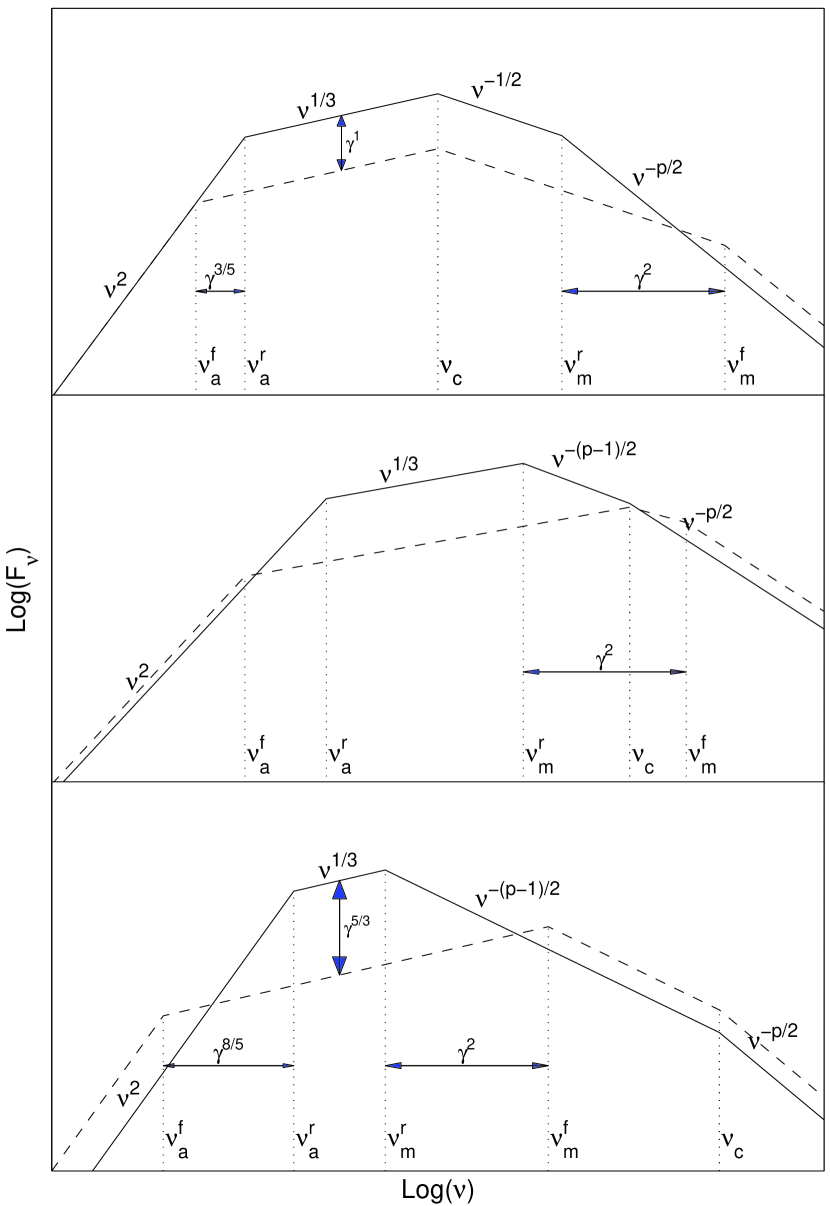
Figure 1: Spectrum of the reverse and forward shocks with synchrotron peaks at $\nu_{m}^{r}$ and $\nu_{m}^{f}$, synchrotron self-absorption frequencies $\nu_{a}^{r}$ and $\nu_{a}^{f}$ and cooling frequency $\nu_{c}$ (same for both, assuming $\epsilon_{B}^{f}=\epsilon_{B}^{r}$), for an electron injection spectrum $\propto\gamma^{-p}$. Top: both shocks fast cooling. Middle: reverse slow, forward fast cooling. Bottom: both slow cooling.

References

- Akerlof, et al. (1999) Akerlof, C., et al., 1999, Nature, 398, 389
- Blandford & McKee (1976) Blandford, R.D. & McKee, C., 1976, Phys.Fluids 19, 1130
- Best & Sari (2000) Best, P. & Sari, R., 2000, Phys.Fluids in press.
- Fenimore & Ramirez-Ruiz (1999) Fenimore, E.E. & Ramirez-Ruiz, E., 1999, ApJ subm (astro-ph/9909299)
- Galama et al. (1999) Galama, T. et al., 1999, Nature, 398, 394
- (6) Granot, J., Piran, T. & Sari, R., 1999, ApJ, 513, 679
- (7) Granot, J., Piran, T. & Sari, R., 1999, ApJ, 527, 236
- Granot, Piran & Sari (2000) Granot, J., Piran, T. & Sari, R., 2000, ApJL submitted
- Kulkarni et al. (1999) Kulkarni, S., et al., 1999, Nature, 398, 389
- Kumar & Piran (1999) Kumar, P. & Piran, T., 1999, astro-ph/9906002
- (11) Mészáros , P. & Rees, M.J., 1997a, ApJ, 476, 232
- Mészáros , Rees & Wijers (1998) Mészáros , P., Rees, M.J. & Wijers, R., 1998, ApJ, 499, 301
- Mészáros & Rees (1999) Mészáros , P. & Rees, M.J. 1999, MNRAS 306, L39
- Panaitescu, Mészáros & Rees (1998) Panaitescu, A., Mészáros , P. & Rees, MJ, 1998, ApJ, 503, 314
- Rees & Mészáros (1998) Rees, M.J. & Mészáros , P., 1998, ApJ, 496, L1
- Sari, (1998) Sari, R. , 1998, ApJ, 494, L49
- Sari, Piran & Narayan (1998) Sari, R., Piran, T. & Narayan, R., 1998, ApJ, 497, L17
- (18) Sari, R. & Piran, T., 1999, ApJ, 520, 641
- (19) Sari, R. & Piran, T., 1999b, ApJ, 517, L109
- Wijers, Rees & Mészáros (1997) Wijers, R.A.M.J., Rees, M.J. & Mészáros , P., 1997, MNRAS, 288,
- Wijers & Galama (1999) Wijers, R.A.M.J. & Galama, T., 1999, ApJ, 523, 177.