Two-dimensional models of hydrodynamical accretion flows into black holes

Abstract

We present a systematic numerical study of two-dimensional axisymmetric accretion flows around black holes. The flows have no radiative cooling and are treated in the framework of the hydrodynamical approximation. The models calculated in this study cover the large range of the relevant parameter space. There are four types of flows, determined by the values of the viscosity parameter $\alpha$ and the adiabatic index $\gamma$: convective flows, large-scale circulations, pure inflows and bipolar outflows. Thermal conduction introduces significant changes to the solutions, but does not create a new flow type. Convective accretion flows and flows with large-scale circulations have significant outward-directed energy fluxes, which have important implications for the spectra and luminosities of accreting black holes.

Subject headings: Accretion, accretion disks — conduction — convection — hydrodynamics — turbulence

1 Introduction

In this paper we present the numerical study of global properties of hydrodynamical black hole accretion flows with a very inefficient radiative cooling. Such flows, coined ADAFs by Lasota (1996, 1999), are thought to be present in several astrophysical black hole candidates, in particular in low mass X-ray binaries and in some active galactic nuclei. Observed properties of ADAFs may be directly connected to black hole physics, and for this reason ADAFs have recently attracted a considerable attention (for reviews see e.g. Kato, Fukue & Mineshige 1998; Abramowicz, Björnsson & Pringle 1998; Narayan 1999).

The radiation losses are unimportant for dynamics as well as for thermal balance of ADAFs, and therefore the details of radiative processes are not crucial. Radiative feed-back into hydrodynamics is negligible and may be treated as a small perturbation. Abramowicz et al. (1995) and in more details Chen et al. (1995) described accretion disks solutions in the parameter space ($\dot{m}$, $\tau$, $\alpha$), where $\dot{m}=\dot{M}/\dot{M}_{Edd}$ is the accretion rate expressed in the Eddington units, $\tau$ is the optical depth and $\alpha$ is the viscosity parameter. In this space ADAFs exist in two regimes (as anticipated by Rees et al. 1982):

(1) ADAFs with $\tau\gg 1$ have super-Eddington accretion rates, $\dot{m}>1$. Radiation is trapped inside the accretion flow (Katz 1977; Begelman 1978). To this category belong slim accretion disks (Abramowicz et al. 1988) which have a vertical scale comparable the corresponding radius.

(2) ADAFs with $\tau\ll 1$ have very sub-Eddington accretion rates, $\dot{m}\ll 1$. These flows have been first investigated by Ichimaru (1977), but the recent interest in them was generated mostly by the works of Narayan and his collaborators, after important aspects of nature of the flows had been explained by Narayan & Yi (1994, 1995b) and Abramowicz et al. (1995).

The most important parameters for the physics of ADAFs are the viscosity parameter $\alpha$ and the adiabatic index $\gamma$. The latter parameter determines the regime of ADAFs through the equation of state. The parameters $\tau$ and $\dot{m}$ are not important: ADAFs have either $\tau\gg 1$ and $\dot{m}>1$, or $\tau\ll 1$ and $\dot{m}\ll 1$. There are no strong observational or theoretical limits for $\alpha$ and $\gamma$, and therefore, at present, one needs to construct models in wide ranges of them. In this paper we have constructed models for $10^{-2}\leq\alpha\leq 1$ and $\gamma=4/3$, $3/2$, $5/3$. Our models are time dependent and fully 2-D: all components of forces and all components of viscous stresses are included in the calculations. To minimize the influence of the outer boundary condition onto the flow structure, we consider the solutions in the large radial range, $3r_{g}\leq r\leq 8\times 10^{3}r_{g}$, where $r_{g}=2GM/c^{2}$ is the gravitational radius of the central black hole with mass $M$. We have found that the properties of ADAFs depend mainly on the viscosity, i.e. on $\alpha$, and also, but less strongly, on the adiabatic index $\gamma$. Four types of accretion flows can be distinguished (see Figure 1).

(i) Convective flows. For a very small viscosity, $\alpha\lesssim 0.03$, ADAFs are convectively unstable, as predicted by Narayan & Yi (1994) and confirmed in numerical simulations by Igumenshchev, Chen & Abramowicz (1996), Stone, Pringle & Begelman (1999) and Igumenshchev & Abramowicz (1999). Axially symmetric convection transports the angular momentum inward rather than outward, for a similar reason as that described by Stone & Balbus (1996) in the context of turbulence: if there are no azimuthal gradients of pressure, turbulence tries to erase the angular momentum gradient. This property of convection governs the flow structure, as it was shown for ADAFs by Narayan, Igumenshchev & Abramowicz (2000) and Quataert & Gruzinov (2000). There are small scale circulations, with the matter fluxes considerably greater than that entering the black hole. Convection transports a significant amount of the dissipated binding energy outward. No powerful outflows are present.

(ii) Large-scale circulations. For a larger, but still small viscosity, $\alpha\sim 0.1$, ADAFs could be both stable or unstable convectively, depending on $\alpha$ and $\gamma$. The flow pattern consists of the large-scale ($\sim r$) meridional circulations. No powerful unbound outflows are present. In some respect this type of flow is the limiting case of the convective flows in which the small scale motions are suppressed by larger viscosity.

(iii) Pure inflows. With an increasing viscosity, $\alpha\simeq 0.3$, the convective instability dies off. Some ADAFs (with $\gamma\simeq 3/2$) are characterized by a pure inflow pattern, and agree in many aspects with the self-similar models (Gilham 1981; Narayan & Yi 1994). No outflows are present.

(iv) Bipolar outflows. For a large viscosity, $\alpha\simeq 1$, ADAFs differ considerably from the simple self-similar models. Powerful unbound bipolar outflows are present.

Effects of turbulent thermal conduction have been studied in several simulations. The conduction has an important influence to the flow structure, but it does not introduce a new type of flow.

The paper is organized as follows. In §2 we describe equations, numerical method and boundary conditions. In §3 we present numerical results for models with and without thermal conduction. In §4 we discuss the properties of the solutions and their implications. In §5 we give the final conclusions.

2 Numerical method

We compute ADAFs models by solving the non-relativistic time-dependent Navier-Stokes equations which describe accretion flows in a given and fixed gravitational field:

$${d\rho\over dt}+\rho\nabla\vec{v}=0,$$

$$\rho{d\vec{v}\over dt}=-\nabla P+\rho\nabla\Phi+\nabla{\bf\Pi},$$

$$\rho{de\over dt}=-P\nabla\vec{v}-\nabla\vec{q}+Q.$$

Here $\rho$ is the density, $\vec{v}$ is the velocity, $P$ is the pressure, $\Phi=-GM/r$ is the Newtonian gravitational potential of the central point mass $M$, $e$ is the specific thermal energy, ${\bf\Pi}$ is the viscous stress tensor with all components included, $\vec{q}$ is the heat flux density due to thermal conduction and $Q$ is the dissipation function. The flow is assumed to be axially symmetric. There is no radiative cooling of the accretion gas. We adopt the ideal gas equation of state,

$$P=(\gamma-1)\rho e,$$

and consider only the shear viscosity with the kinematic viscosity coefficient given by

$$\nu=\alpha{c_{s}^{2}\over\Omega_{K}},$$

where $0<\alpha\lesssim 1$, $c_{s}=\sqrt{P/\rho}$ is the isothermal sonic speed and $\Omega_{K}=\sqrt{GM/r^{3}}$ is the Keplerian angular velocity. We assume that the thermal conduction heat flux is directed down the specific entropy gradient,

$$\vec{q}=-\chi\rho T\nabla s,$$

where $s$ is the specific entropy, $T$ is the temperature and $\chi$ is the thermometric conductivity. The formula (2.6) is correct for flows in which the heat conduction is due to either turbulent eddies or diffusion of radiation in the optically thick medium. Other laws of thermal conduction are possible for different heat transfer mechanisms. In numerical models we assume a simplified dependence,

$$\chi=\nu/Pr,$$

where $Pr$ is the dimensionless Prandtl number assumed to be constant in the flow, and $\nu$ is defined by (2.5). In the flows without thermal conduction, i.e. $\chi=0$, one formally has $Pr=\infty$. In the case of turbulent flows the actual value of the Prandtl number is not clearly known and can vary in a wide range, $1\lesssim Pr<\infty$, depending on the nature of turbulence. If the viscosity in turbulent flows is provided mainly by small scale eddies, one can expect $Pr\sim 1$. If the viscosity is due to magnetic stress, the thermal conduction could be significantly suppressed, i.e. $Pr\gg 1$. Note, that for molecular thermal conduction in gases, the Prandtl number is always of the order of unity (e.g. Landau & Lifshitz 1987). In actual calculations, we use

$$\vec{q}=-\chi\left[\nabla(\rho e)-\gamma e\nabla\rho\right],$$

which is equivalent to (2.6).

We split the numerical integration of equations (2.1)-(2.3) into three sub-steps: hydrodynamical, viscous and conductive. The hydrodynamical sub-step is calculated by using the explicit Eulerian finite-difference algorithm PPM developed by Colella & Woodward (1984). The viscous sub-step is solved by applying an implicit method with a direction-splitting when calculating the contributions to equation (2.2). The dissipation function $Q$ in equation (2.3) is calculated explicitly. The conductive sub-step in equation (2.3) is again calculated by an implicit method with a direction-splitting. The time-step $\Delta t$ for the numerical integration is chosen in accordance with the Courant condition for the hydrodynamical sub-step.

We use a spherical grid $N_{r}\times N_{\theta}=130\times 50$ with the inner radius at $r_{in}=3r_{g}$ and the outer radius at $r_{out}=8000r_{g}$. The grid points are logarithmically spaced in the radial direction and uniformly spaced in the polar direction from $0$ to $\pi$. The general-relativistic capture effect, that governs the flow near black hole, is modeled by using an absorbing boundary condition at $r=r_{in}$. We assume no viscous angular momentum and energy fluxes through the inner boundary associated with the ($r\theta$) and ($r\phi$) components of the shear stress. Namely, we assume $d(v_{\theta}/r)/dr=0$ and $d(v_{\phi}/r)/dr=0$ at $r=r_{in}$. Also, the energy flux due to the thermal conduction at $r=r_{in}$ is assumed to be zero. At the outer boundary $r_{out}$ we apply an absorbing boundary condition. The matter can freely outflow through $r_{out}$, but there are no flows from outside.

In the calculations, we assume that mass is steadily injected into the calculation domain from an equatorial torus near the outer boundary of the grid. Matter is injected there with angular momentum equal to $0.95$ times the Keplerian angular momentum. Due to viscous spread, a part of the injected matter moves inwards and forms an accretion flow. The other part leaves the computation domain freely through the outer boundary. We start computations from an initial state in which there is a little amount of mass in the grid. As the injected mass spreads and accretes, the amount of mass within the grid increases. After a time comparable to the viscous time scale at $r_{out}$, the accretion flow achieves a quasi-stationary behaviour, and may be considered to be in a steady state. However, for some models this ‘steady state’ is steady only in the sense of time-averaging: these flows show persistent chaotic fluctuations, at any given point, which do not die out with time.

3 Two-dimension hydrodynamical models

Spatial re-scaling $r\rightarrow x$ together with time re-scaling $t\rightarrow t/(r_{g}/c)$, make solutions of (2.1)–(2.3) independent of the black hole mass $M$. There is also an obvious re-scaling of density $\rho\rightarrow\rho/\dot{M}_{inj}$ that makes the solutions independent of the mass injection rate $\dot{M}_{inj}$. Thus, with fixed boundary conditions, the numerical models are described by the three dimensionless parameters $\alpha$, $\gamma$ and $Pr$. We have calculated a variety of models for different values of these parameters (see Table 1).

3.1 Models without thermal conduction

First, we describe accretion flows with no thermal conduction ($Pr=\infty$). The results of the simulations are summarized in Figure 1 (left panel). Here circles show the location of the computed models in the ($\alpha$, $\gamma$) plane. Empty circles correspond to stable laminar flows. Unstable models with large-scale ($\sim r$) circulation motions are represented by crossed circles. Unstable models with small-scale ($\lesssim r$) convective motions are shown by solid circles. Arrows indicate the presence of powerful outflows or strong inflows in the models. Two outward directed arrows, on the upper and lower of a circle, mean the bipolar outflows, whereas one arrow corresponds to the unipolar outflow. Inward directed arrows indicate that the model has a pure inflow pattern. Models which are not marked by arrows reveal neither powerful outflows, nor pure inflow.

The source of matter in our models has a constant injection rate and locates close to the outer boundary. In a steady state one expects that due to this particular location of the source, most of the material injected into the computational domain escapes through the outer boundary and only a minor part of it accretes into the black hole. Table 2 presents the ratio of the mass accretion rate $\dot{M}_{0}$, measured at the inner boundary, to the mass outflow rate $\dot{M}_{out}$ through the outer boundary for a variety of models. The selected models are both stable and unstable, and we use the time-averaged rates in the case of unstable models. From Table 2 one can see that in most cases the ratio $\dot{M}_{0}/\dot{M}_{out}$ is very small, $\sim 10^{-2}-10^{-3}$, and shows a complicated dependence on $\alpha$ and $\gamma$. The smallest relative accretion rates correspond to the models with a small viscosity (Models J, K and L) and a smaller ratio corresponds to a larger $\gamma$ in these models. A similar dependence of $\dot{M}_{0}/\dot{M}_{out}$ on $\gamma$ can also be seen for other fixed values of $\alpha$. However, Model E demonstrates a peculiar property: the mass accretion rate is about two times larger than the outflow rate. We will discuss later in detail this peculiar model and show that it is closely related to the ‘standard’ self-similar ADAF solutions (Narayan & Yi 1994), whereas other models are either not related to self-similar ADAFs, or related to self-similar ADAFs of a new kind (Narayan et al. 2000; Quataert & Gruzinov 2000).

A small value of the ratio $\dot{M}_{0}/\dot{M}_{out}$ does not indicate powerful unbound outflows. In some models the large outflow rate is only a consequence of our choice of the geometry of matter injection. To confirm this point, we present in Figure 2 a variety of histograms, which show the fraction of matter that outflows behind the outer boundary and has a fixed value of the dimensionless Bernoulli parameter $Be$,

$$Be=\left({1\over 2}v^{2}+W-{GM\over r}\right)\left/{GM\over r}\right..$$

Here $W=\gamma c_{s}^{2}/(\gamma-1)$ is the specific enthalpy. The histograms are shown for Models A, D, G and J, all with fixed $\gamma=5/3$ and different values of $\alpha$. We have used the standard normalization $\sum\Delta\dot{m}_{out}(Be)=1$ in the histograms. The matter with positive $Be$ is gravitationally unbound and can form outflows, whereas the matter with negative $Be$ is gravitationally bound and cannot escape to a large radial distance. One can see in Figure 2 that the high viscosity flows (Models A and D) form powerful unbound outflows with positive and large $Be$ on average, and only a minor part of the outflowing matter ($\sim 20\%$) is gravitationally bound. In the low viscosity flows (Models G and J) most of the matter that moved through the outer boundary has $Be<0$ and thus it remains gravitationally bound and cannot form powerful outflows. We have found a similar situation with respect to formation of bound/unbound outflows in models with different $\gamma$. In general, flows with low $\alpha$ are bound and have no powerful outflows.

As we explained in Introduction, the numerical models of ADAFs could be divided into four types that are characterized by different flow patterns. We shall now describe the properties of the flows of the various types.

3.1.1 Bipolar outflows

The high viscosity ($\alpha=1$) Models A, B, C and moderate viscosity ($\alpha=0.3$) Model D are stationary, symmetric with respect to the equatorial plane, and show a flow pattern with equatorial inflow and bipolar outflows. In Models A, B and C the mass is strongly concentrated towards the equatorial plane, and the flow patterns depend weakly on $\gamma$. The angular momentum is significantly smaller than the Keplerian one, and the pressure gradient force plays a major role in balancing gravity. We discuss here two representative high viscosity Models A ($\gamma=5/3$) and C ($\gamma=4/3$). Model B has properties somewhat between those of Models A and C.

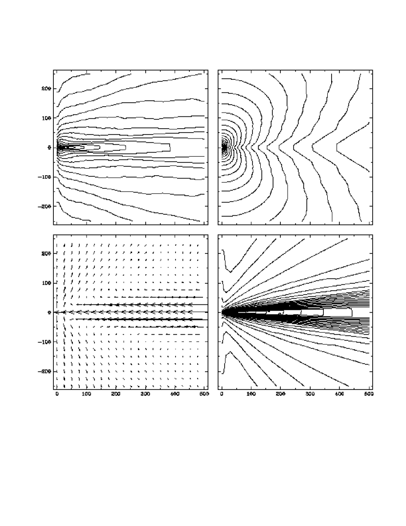
Figure 4: Some selected properties of Model C ($\alpha=1$, $\gamma=4/3$ and $Pr=\infty$) in the meridional cross-section. The difference of this model from Model A presented in Figure 3 appears mostly in the distributions of the Mach number ${\cal M}$ (lower right panels). Model C shows supersonic (${\cal M}>1$) equatorial inflow. The thick line in the distribution of ${\cal M}$ corresponds to the value ${\cal M}=1$. Other details as in Figure 3.

Figures 3 and 4 present selected properties of Models A and C, respectively, in the meridional cross-section. Four panels in each figure show the distributions of density $\rho$ (upper left), pressure $P$ (upper right), momentum vectors $\rho\vec{v}$ multiplied by $r$ (lower left), and Mach number ${\cal M}=\sqrt{v_{r}^{2}+v_{\theta}^{2}}/\sqrt{\gamma}c_{s}$ (lower right). The correspondent distributions in Figures 3 and 4 are almost identical except the distributions of ${\cal M}$. In Model A (as well as in Models B and D) the flow is everywhere subsonic up to the inner absorbing boundary at $3r_{g}$. In the equatorial inflow the radial profile of ${\cal M}$ is flat and reaches the maximum value ${\cal M}\simeq 0.7$. In Model C the equatorial inflow is supersonic in a large range of radii inside about $3\times 10^{3}r_{g}$. The equatorial values of ${\cal M}(r)$ increase with decreasing radius and take the maximum value ${\cal M}=2.4$ at the inner boundary. Thus, the presence of the supersonic or subsonic inflow in high viscosity models depends on the value of $\gamma$, which controls the ‘hardness’ of the equation of state (2.4). We note that in purely radial supersonic inflows the viscous torque cannot be efficient because of a reduction of the upstream transport of viscous interactions. This effect was referred as a ‘causal’ effect (Popham & Narayan 1992). Due to this effect the supersonic inflow in geometrically thin and centrifugally supported accretion disks is possible only in the innermost region with radius close to the radius of the last stable black hole orbit $r_{s}$. However, in the case of Model C the viscous interaction between the supersonic equatorial inflow and the outflowing material plays an important role. The expansion velocities in the outflows are subsonic, and there is no problem with causality. In this case the inflow can be supersonic for radii $r\gg r_{s}$.

To quantitatively characterize the process of bipolar outflows we have estimated the ‘mass inflow rate’ $\dot{M}_{in}(r)$ by adding up all the inflowing gas elements (with $v_{r}<0$) at a given radius $r$, and compared $\dot{M}_{in}$ with the net accretion rate $\dot{M}_{0}$. The results are shown in Figure 5 for Models A (solid line), C (dotted line) and D (dashed line). The curves do not show power-law dependences, because they do not look like straight lines on the log–log plot. From Figure 5 one can see that $\dot{M}_{in}$, and correspondingly the ‘mass outflow rate’, $\dot{M}_{out}=\dot{M}_{in}-\dot{M}_{0}$, strongly depend on $\gamma$ at a fixed $\alpha$. In the case of Model A only about $1/7$ of matter that inflows at $r=1000r_{g}$ reaches the black hole, whereas in the case of Model C the fraction is about $1/2$. Model D shows that a reduction of $\alpha$ by three times, with respect to the one for Model A, results in $\simeq 2-3$ times suppression of the mass outflow rate $\dot{M}_{out}$ in the radial range of $\sim 10^{2}-10^{3}r_{g}$. Models with smaller $\gamma$ show the tendency of larger suppression of $\dot{M}_{out}$ with decreasing $\alpha$.

It is interesting to compare the behaviour of the dimensionless quantities

$$\lambda={1\over\dot{M}_{in}\ell_{K}}\left(\dot{M}_{in}\ell+2\pi r^{3}\int\Pi_{r\phi}\sin\theta d\theta\right),$$

and

$$\epsilon={1\over\dot{M}_{in}v_{K}^{2}}\left(\dot{E}_{adv}+\dot{E}_{visc}\right),$$

in our models with prediction of self-similar solutions in which $\lambda$ and $\epsilon$ are constants (see Blandford & Begelman 1999). In (3.2) and (3.3) we have used the following notation,

$$\dot{E}_{adv}=2\pi r^{2}\int\rho v_{r}\left({v^{2}\over 2}+W+\Phi\right)\sin\theta d\theta,$$

$$\dot{E}_{visc}=2\pi r^{2}\int(v_{r}\Pi_{rr}+v_{\theta}\Pi_{r\theta}+v_{\phi}\Pi_{r\phi})\sin\theta d\theta,$$

$\ell=v_{\phi}r\sin\theta$ is the specific angular momentum, and $v_{K}=\Omega_{K}r$ and $\ell_{K}=\Omega_{K}r^{2}$ are the Keplerian angular velocity and angular momentum, respectively. Integration in (3.2)-(3.5) has been taken over those angles $\theta$ for which $v_{r}<0$. In our models $\lambda$ and $\epsilon$ are changed with radius. The functions $\lambda(r)$ and $\epsilon(r)$ are plotted in Figure 6 by the solid, dotted and dashed lines for Models A, C and D, respectively. Analysing the dependences in Figure 6 as well as the behaviour of $\dot{M}_{in}$ in Figure 5, one conclude that Models A, C and D do not reveal the self-similar behaviour.

Figures 7 and 8 show the angular structure (in the $\theta$-direction) in Model A and D, respectively, at four radial positions of $r=30r_{g}$ (long-dashed lines), $100r_{g}$ (dashed lines), $300r_{g}$ (dotted lines) and $1000r_{g}$ (solid lines). The angular distribution of density demonstrates a considerable concentration of matter towards the equatorial plane in high viscosity Model A. The concentration is less significant in the case of moderate viscosity Model D. The models show quite flat distributions of angular velocity $\Omega$, especially at smaller $r$. The radial velocities $v_{r}$ are negative in the equatorial inflowing regions, where the mass concentration takes place. The wide polar regions are filled by the unbound outflowing matter with positive $v_{r}\gtrsim v_{K}$. The polar outflows are less effectively accelerated in Model D, and it results in a reduction of the mass outflow rates $\dot{M}_{out}$ in comparison with those of Model A (dashed and solid lines in Figure 5, respectively). In the polar regions $c_{s}/v_{K}\gtrsim 1$, whereas in the inflowing part one has $c_{s}/v_{K}<1$. Note, that the ratio $c_{s}/v_{K}$ equals to the relative thickness of the accretion flow in the vertically averaged accretion disk theory (e.g. Shakura & Sunyaev 1973), $h/r=c_{s}/v_{K}$. In accretion disks one has $h/r\lesssim 1$. The case $h/r\gtrsim 1$ corresponds to a thermally expanded unbound gas cloud. Models B and C demonstrate angular structures qualitatively similar to that of Model A.

Figure 9 shows the averaged radial structure for a variety of models. Models A, C and D are represented by the solid, dotted and dashed lines, respectively. All plotted quantities, $\rho$, $\Omega$, $v_{r}$, $c_{s}$, have been averaged over the polar angle $\theta$ with the weighted function $\rho$, except for $\rho$ itself. The density and sonic velocity profiles in the models can approximately be described by radial power-laws, with $\rho\propto r^{-1}$ and $c_{s}\propto r^{-1/2}$. The radial velocity is about $v_{r}\propto r^{-1}$ in the case of Models A and D, but does not show any distinguished power-law dependence in the case of Model C. The latter model shows faster increase of the radial velocity with decreasing radius. The most significant difference between the high and moderate viscosity models can be seen in the radial profiles of $\Omega$. The angular velocity $\Omega$ shows quite unexpected behaviour in the case of high viscosity Models A and C. In Model A, $\Omega\propto r^{-1/2}$ in all ranges of the radii. This radial dependence is significantly flatter than the one for the Keplerian angular velocity, $\Omega_{K}\propto r^{-3/2}$. In Model C, $\Omega\propto r^{-1/2}$ in the outer region, at $r\gtrsim 10^{3}r_{g}$, and $\Omega\propto\Omega_{K}\propto r^{-3/2}$ in the inner region, at $r\lesssim 10^{2}r_{g}$. The steeper dependence of $\Omega(r)$ in the inner region of Model C could be due to the equatorial supersonic inflow (see Figure 4, lower right panel). In moderate viscosity Model D, the angular velocity profile is not surprising, it is quite close to the Keplerian one.

3.1.2 Pure inflows

As we noted earlier, Model E demonstrates some peculiar properties. The model is stable and does not form outflows except very close to the outer boundary, at $r\gtrsim 4000r_{g}$. Figure 10 shows some selected properties of Model E in the meridional cross-section. The flow pattern looks very similar to the one for the spherical accretion flow. However, contrary to spherical flows, the rotating accretion flow in Model E has a reduced inflow rate at the equatorial and polar regions (compare vectors in the lower left panel of Figure 10) and a corresponding local decrease of Mach number there (Figure 10, lower right panel). The net radial energy flux is close to zero for $r\lesssim 10^{3}r_{g}$ in this model; the inward advection of energy balances the outward-directed energy flux due to viscosity (see plot for $\epsilon$ in Figure 6, long-dashed line). Such a balance of the inward and outward energy fluxes in Model E coincides with a property of the self-similar ADAF solutions, in which $\epsilon=0$. An other property of the self-similar ADAFs is that $\lambda=0$. The latter property is a consequence of the assumption that the inner boundary located at $r=0$, and there is a zero outward flux of angular momentum. In reality, however, the inner boundary locates at a finite radius, and there must be a non-zero outward flux of angular momentum $\approx\dot{M}_{0}\ell(r_{in})$. In this case $\lambda$ is a function of radius, $\lambda(r)\propto\ell_{K}^{-1}\propto r^{-1/2}$. Model E confirms the latter dependence in a wide range of radii, at $r\lesssim 2\times 10^{3}r_{g}$, as can be seen from the $\lambda(r)$ plot in the lower panel of Figure 6 (long-dashed line). It is interesting to note that Model D demonstrates a similar behaviour of $\lambda(r)$ (dashed line in the lower panel of Figure 6) in the innermost part, at $r\lesssim 30r_{g}$, where the outflow rate $\dot{M}_{out}$ is small (see Figure 5).

The radial and angular structure of Model E can be seen in Figures 9 (long-dashed lines) and 11. The radial profiles of the $\theta$-averaged $\rho$, $\Omega$ and $c_{s}$ are very close to those for the self-similar ADAFs: $\rho\propto r^{-3/2}$, $\Omega\propto r^{-3/2}$ and $c_{s}\propto r^{-1/2}$. But, the angular profiles of them do not correspond to any of the two-dimensional self-similar solutions found by Narayan & Yi (1995a). The discrepancy is connected with a reduction of mass inflow rate in the equatorial region clearly seen in Model E. The parameter $Be$ is positive in the inner region of Model E, at $r\lesssim 10^{3}r_{g}$, and there are no outflows.

3.1.3 Large-scale circulations

Models F, G, H and I with large-scale circulations have a moderate viscosity, $0.1\lesssim\alpha\lesssim 0.3$. In the ($\alpha$, $\gamma$) plane they locate on both sides of the line that separates the stable and unstable flows (see Figure 1, left panel). Below we discuss representative stable Model G and unstable Models F and I.

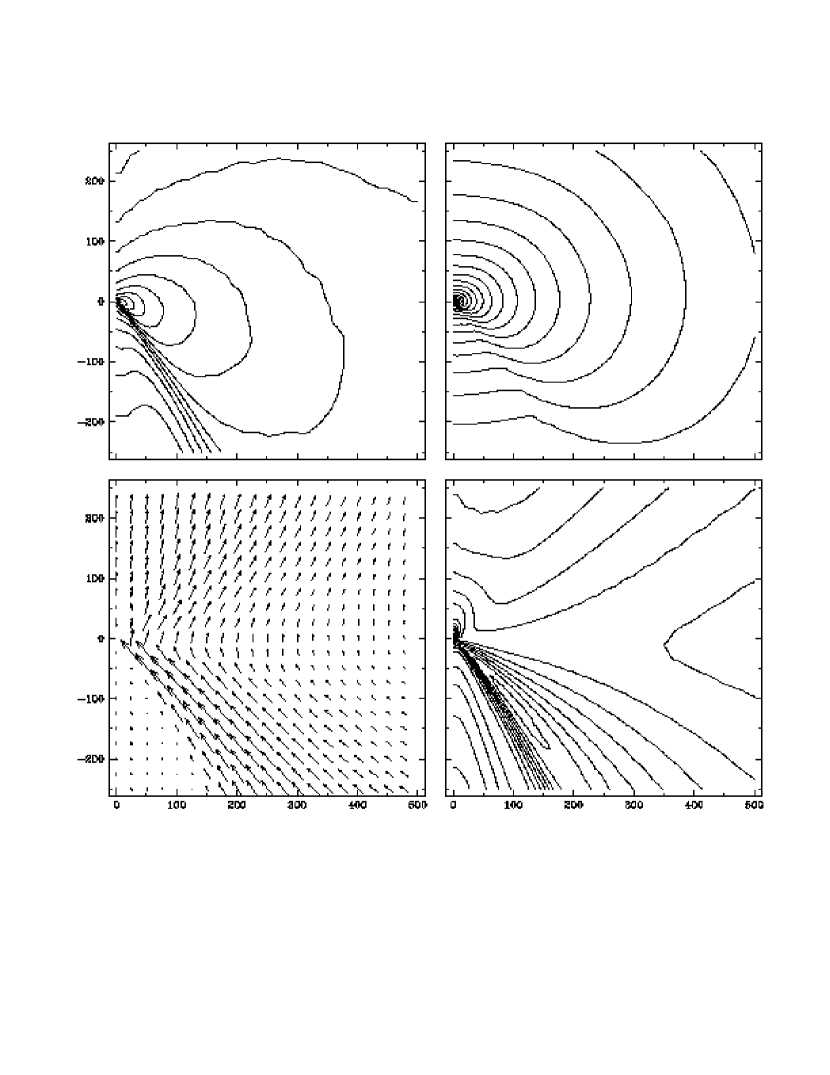
Figure 12: Some selected properties of Model G ($\alpha=0.1$, $\gamma=5/3$ and $Pr=\infty$) in the meridional cross-section. See the caption of Figure 3 for details. The inner part of the global circulation cell with a unipolar outflow directed to the upper hemisphere is seen in momentum vectors (lower left). The polar funnel in the lower hemisphere is filled by low density matter. The thick line in the distribution of the Mach number (lower right) corresponds to the maximum contour ${\cal M}=0.8$.

The flow pattern for stable Model G is presented in Figure 12. In the lower left panel of Figure 12 one can see the inner part of a meridional cross-section of the global circulation cell which has a torus-like form in three dimensions. The polar outflow in the upper hemisphere becomes supersonic from $\sim 1000r_{g}$ outward. The polar funnel in the lower hemisphere filled up by low-density matter is clearly seen in the distributions of density (upper left), pressure (upper right) and Mach number (lower right). The low-density matter in the funnel forms an accretion flow at small $r$ and an outflow at larger $r$. The boundary between these inflowing and outflowing parts is variable and determines the supersonic/subsonic accretion regime in the funnel. At the particular moment shown in Figure 12 the boundary between the inflow and outflow in the funnel is located at small $r$ and the accretion flow is mostly subsonic. Figure 13 shows the angular structure of the flow in Model G. The equatorial asymmetry of the flow pattern introduces the asymmetry in the angular profiles of all quantities shown. Note the impressive similarity of the profiles at different radial distances except regions close to the poles.

Snapshots of the unstable Models F and I are given in Figure 14, left and right panels, respectively. Model F has a stable global flow pattern dominated by an unipolar circulation motion. The flow is quasi-periodically perturbed by growing hot convective bubbles. These bubbles originate in the innermost part of the accretion flow close to the equatorial plane. They are hotter and lighter than the surrounding matter, and the Archimedes buoyancy forces them to move outward. During the motion, the bubbles are heated up further due to viscous dissipation and migrate from the equatorial region to the upper hemisphere. In Figure 14 (left) one can see the growing bubble in the density contours inside $r\simeq 500r_{g}$. The structure seen in the upper polar region at $r\simeq 2000r_{g}$ is a ‘tail’ of the previous bubble. Less viscous Model I does not show a regular flow pattern. The hot convective bubbles outflow quasi-periodically in both the upper and lower hemispheres without a preferable direction. Figure 14 (right) shows sequences of the convective bubbles in the polar regions of both hemispheres. The regular flow pattern with the symmetric bipolar outflows and equatorial inflow is seen only through the time averaging in Model I.

3.1.4 Convective flows

All our low viscosity models with $\alpha\lesssim 0.03$ are convectively unstable independently of $\gamma$. They show complicated time-dependent flow patterns which consist of numerous vortices and circulations. The snapshot of such a behaviour of accretion flow in the case of Model M is presented in Figure 15 (left). It demonstrates non-monotonic distributions of density and velocity in the innermost part of the flow. In spite of the significant time-variability of the accretion flow we have found a tendency towards formation of temporal coherent structures which look like convective cells extended in the radial direction. In these structures, the inflowing streams of matter are sandwiched in the $\theta$-direction by the outflowing streams. These structures can be seen in the velocity vectors and in the characteristic radial features of the density distribution in the left panel of Figure 15. The time-averaged flow patterns are smooth and do not demonstrate small-scale features. Figure 15 (right) shows the time-averaged distributions of the density and momentum vectors of Model M. In the picture one can clearly see that the accretion is suppressed in the equatorial sector and the mass inflows concentrate mainly along the upper and lower surfaces of the torus-like accretion disk.

Figure 16 shows the angular structure of the time-averaged flow from Model M. All quantities have been averaged over about $44$ periods of the Keplerian rotation at $r=100r_{g}$. The angular profiles of density reach their maximum values at the equator and decrease towards the poles. The profiles have an almost identical form at each radius. The similarity of the angular profiles at different $r$ can be see as well in the variables $\Omega$, $v_{r}$ and $c_{s}$, except in the regions which are close to the poles. The averaged radial velocity is almost zero over most of the $\theta$-range. It is only close to the poles that we have non-zero velocities (for $r\lesssim 300r_{g}$ they are negative and for larger $r$ they are positive). The polar inflows are highly supersonic in the low viscosity models as can be seen by comparing the values of $v_{r}$ and $c_{s}$ from the lower left and lower right panels of Figure 16.

Figure 17 shows the radial structure of the time-averaged flows in Models J (dotted lines), K (dashed lines), L (long-dashed lines) and M (solid lines). It uses the same $\theta$-averaging as in Figure 9. In all models, the variables $\Omega$ and $c_{s}$ can be described by a radial power-law, with $\Omega\propto r^{-3/2}$ and $c_{s}\propto r^{-1/2}$, in the radial range $\sim 10-10^{3}r_{g}$. The radial density profile can also be approximated by a power-law, $\rho\propto r^{-\beta}$, where the index $\beta$ varies from $\beta\approx 0.5$ for Models J and M to $\beta\approx 0.7$ for Models K and L. The radial velocities are connected to the density profiles by the relation $v_{r}\propto r^{-2}\rho^{-1}\propto r^{\beta-2}$ with good accuracy. Such a fast increase of $v_{r}$ inward, with respect to the free-fall velocity, $v_{ff}\propto r^{-1/2}$, means that $v_{r}$ is very small at large radii in comparison with the predictions of the ‘standard’ self-similar ADAF solutions, for which $v_{r}\propto v_{ff}\propto r^{-1/2}$. The angular velocities are close to the Keplerian ones everywhere, and the $\Omega(r)$ profiles for Models K, M, L have a super-Keplerian part at the innermost region, which is typical for thick accretion disks.

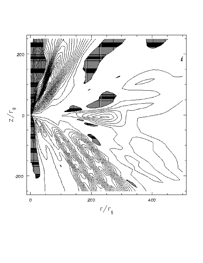
Figure 18: The ($r\phi$)-component of the Reynolds stress tensor normalized to the square of the Keplerian velocity, $\langle v_{r}^{\prime}v_{\phi}^{\prime}\rangle/v_{K}^{2}$, in the meridional cross-section of the convectively unstable Model K ($\alpha=0.01$, $\gamma=5/3$, $Pr=\infty$). The contours are given with the step $\Delta=2.5\times 10^{-4}$. Regions with positive values of the Reynolds stress are shown in grey. It is clearly seen that the Reynolds stress is mostly negative in the bulk of the flow. This means that the angular momentum is transported inward by the convection motions.

The most interesting and important property of the low viscosity models is that the convection transports angular momentum inward rather than outward, as it does in the case of ordinary viscosity. The direction of the angular momentum transport is determined by the sign of the ($r\phi$)-component of the Reynolds stress tensor, $\tau_{r\phi}=\langle v_{r}^{\prime}v_{\phi}^{\prime}\rangle$, where $v_{r}^{\prime}$, $v_{\phi}^{\prime}$ are the velocity fluctuations and $\langle...\rangle$ means time-averaging. Negative/positive sign of $\tau_{r\phi}$ corresponds to inward/outward angular momentum transport. Figure 18 shows the distribution of $\tau_{r\phi}$ in the meridional cross-section of Model M. It is clearly seen that $\tau_{r\phi}$ is negative in most of the flow, and thus convective motions transport angular momentum inward on the whole.

All low viscosity models have negative, volume averaged, $Be$ in all ranges of the radii. Only temporal convective blobs and narrow (in the $\theta$-direction) regions with outflowing matter at the disk surfaces show positive $Be$.

Our numerical results for the low viscosity models agree with those calculated in our earlier papers (Igumenshchev et al. 1996; Igumenshchev & Abramowicz 1999), and are very similar to those obtained later by Stone et al. (1999). The models of Stone et al. (1999) are convectively unstable and the time-averaged radial inward velocity is significantly reduced in the bulk of the accretion flows. Stone et al. (1999) have checked several radial scaling laws for the viscosity and have found the same radial dependence of the time-averaged quantities ($\rho$, $\Omega$ and $c_{s}$), as those presented here, in the case of $\nu\propto r^{1/2}$, which is analogous to the $\alpha$-prescription (2.5).

3.2 Models with thermal conduction

We have assumed the Prandtl number $Pr=1$ in the models with thermal conduction (see Table 1). The thermal conduction does not introduce qualitatively new types of flow patterns in addition to those that were discussed in §3.1. However, it leads to important quantitative differences. Firstly, the thermal conduction makes the contrasts of specific entropy smaller, which leads to a suppression of the small-scale convection in the low and moderate viscosity models. Secondly, the thermal conduction acts as a cooling agent in the outflows, reducing or even suppressing them in the models of moderate viscosity. Calculations that include thermal conduction cover a smaller region in the ($\alpha$, $\gamma$) plane than those of the non-conductive models. Figure 1 (right panel) summarizes some properties of the models with thermal conduction. All computed models are stable. We have found only two types of flow patterns: pure inflow (like in Model E) for all models with $\alpha=0.3$, and global circulation (like in Model G) for models with smaller $\alpha$.

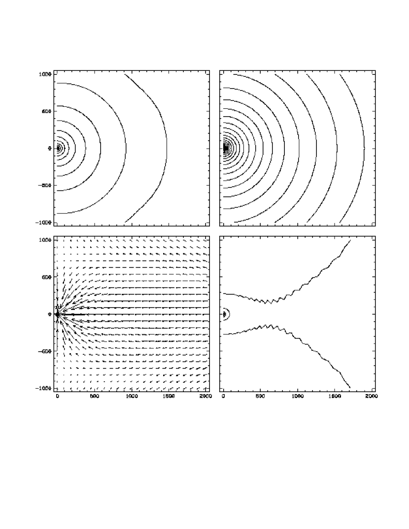
Figure 19: Some selected properties of Model N with thermal conduction ($\alpha=0.3$, $\gamma=5/3$ and $Pr=1$) in the meridional cross-section. See the caption of Figure 3 for details. The flow pattern is almost spherical at $r\lesssim 500r_{g}$. There are two stagnation points at $r\simeq 800r_{g}$, which divide the inflows and outflows in the polar directions (lower left panel).

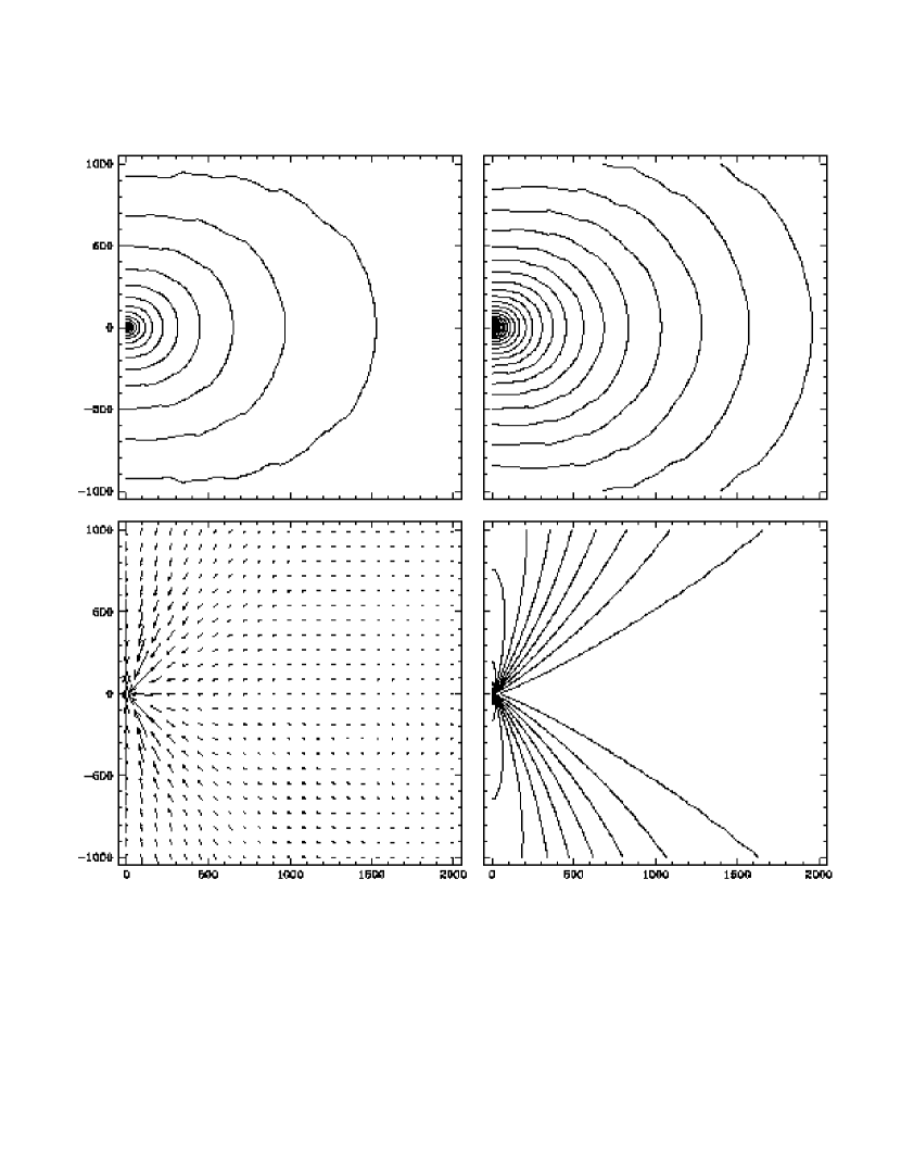
Figure 20: Some selected properties of Model P with thermal conduction ($\alpha=0.3$, $\gamma=4/3$ and $Pr=1$) in the meridional cross-section. See the caption of Figure 3 for details. The inward mass flux is concentrated in the polar directions, similar to the situation in Model E (compare with Figure 10). The thick line in the distribution of the Mach number (lower right) corresponds to ${\cal M}=1$.

Figures 19 and 20 show the two-dimensional structure of Models N and P, respectively, in the meridional cross section. Distributions of density and pressure are almost spherical in both models. Important differences between the models can be seen in the distribution of the momentum vectors (lower left panel) and the Mach number (lower right panel). In Model N the momentum vectors are distributed almost spherically at $r\lesssim 500r_{g}$. At $r\simeq 800r_{g}$ in the polar directions there are two stagnation points which divide inflows from outflows. The distribution of the Mach number is flat, and the flow is significantly subsonic everywhere. In Model P the inward mass flux spreads in the wide ($\sim 45^{\circ}$) polar regions. The equatorial inflow is relatively small. The distribution of the Mach number in Model P has an equatorial minimum and increases towards the poles. At $r\lesssim 200r_{g}$ the polar inflows are supersonic.

Figure 21 presents the radial structure of the flow in Models N (dashed lines), O (long-dashed lines) and P (dotted lines). The density profiles can be approximated by a radial power-law, $\rho\propto r^{-\beta}$, where the index $\beta\approx 1$ for Model N, and $\beta\approx 1.5$ for Models O and P. The profiles of $\Omega(r)$ show a different behavior for each model. In Model N the values of $\Omega$ is significantly reduced with respect to $\Omega_{K}$ in the inner region, $r\lesssim 10^{3}r_{g}$. In Models O and P the drop of $\Omega$ is less significant. The ratio of $\Omega/\Omega_{K}$ goes to a limiting value in the latter models: $\Omega/\Omega_{K}\simeq 0.6$ in the case of Model P and $\simeq 0.3$ in the case of Model O. The radial inward velocities increase with decreasing $\gamma$ in the sequence of models from N to O and P, and is well described by the power-law $v_{r}\propto r^{\beta-2}$. The profiles of $c_{s}(r)$ are weakly changed from model to model.

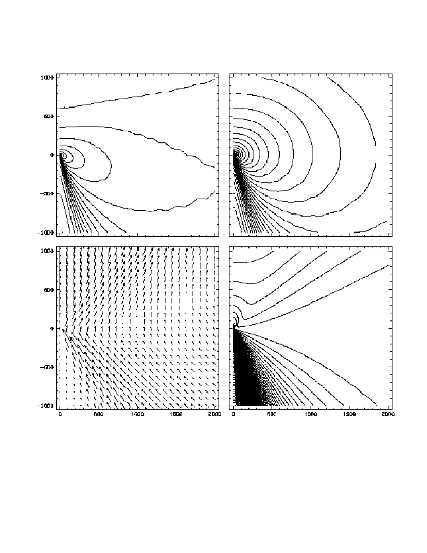
Figure 22: Some selected properties of Model Q with thermal conduction ($\alpha=0.1$, $\gamma=5/3$ and $Pr=1$) in the meridional cross-section. See the caption of Figure 3 for details. The flow pattern is similar to that of Model G (see Figure 12). The thick line in the distribution of the Mach number (lower right) corresponds to ${\cal M}=1$.

Models Q, R and S have almost identical flow patterns and show weak dependence on $\alpha$ and $\gamma$. As an illustrative example we present the flow pattern of Model Q in Figure 22. Like in the case of Model G discussed in §3.1.3 these models form stable global circulations. Contrary to what is seen in Model F, however, these models have a more pronounced accretion funnel in the lower hemisphere, with a highly supersonic matter inflow. Figure 23 shows the angular structure of Model Q. The comparison of this models with the properties of Model G in Figure 13 does not indicate significant quantitative differences in the flow structure except in the narrow polar regions.

4 Discussion

The properties of ADAFs are often discussed in terms of one-dimensional (1D) vertically averaged analytic and numerical models. The comparison of our two-dimensionl (2D) models and 1D models of ADAFs constructed up to date show important qualitative differences, which we would like to stress here. Firstly, the 1D simulations of high and moderate viscosity ($0.1\lesssim\alpha\lesssim 1$) flows cannot reproduce bipolar outflows and large-scale circulations due to obvious, intrinsic limitations of the vertically averaged approach. Only for the pure inflow models the 1D approach could be adequate. However, ADAFs with pure inflows are realized only in a very small range of the parameters $\alpha$ and $\gamma$ and therefore such a type of the flow is not general. Secondly, the low viscosity ($\alpha\lesssim 0.1$) 1D models of ADAF constructed previously had not accounted at all, or had not accounted in all important details, the effects of convection. 2D models show that the convection governs the structure of the low viscosity flows and significantly influences predicted observational properties of them. Future low viscosity 1D ADAF models should account for the convection with all the important details (see Narayan et al. 2000).

Convective accretion flows are quite different from the ‘standard’ self-similar ADAF solutions in several points. Firstly, convective flows have a flattened density profile, $\rho\propto r^{-\beta}$ with $\beta\simeq 0.5$–$0.7$ slightly dependent on $\gamma$, whereas $\beta=-3/2$ in the case of the self-similar ADAFs (Narayan & Yi 1994). Secondly, there is a net outward energy flux in these flows provided by convective motions, whereas the self-similar ADAFs have a zero net energy flux. The amount of energy transported outward by convections is $\sim 10^{-2}\dot{M}_{0}c^{2}$, and the value only moderately depends on $\alpha$ and $\gamma$. These effects have important implications for the spectra and luminosities of accreting black holes. Indeed, since $\rho\propto r^{-1/2}$ and $T\propto r^{-1}$, the bremsstrahlung cooling rate per unit volume varies as $Q_{br}\propto\rho^{2}T^{1/2}\propto r^{-3/2}$ in the case of convective flows, and $Q_{br}\propto r^{-7/2}$ in the case of self-similar ADAFs. Integrating $Q_{br}$ over a spherical volume one can demonstrate that most of the energy losses in convective accretion flows occurs on the outside, whereas most of the energy losses in self-similar ADAFs takes place in the innermost region. Recent analytic works by Narayan et al. (2000) and Quataert & Gruzinov (2000) have provided considerable insight into properties of accretion flows with convection. The analytic analysis is based on the ansatz (confirmed by our previous and present numerical simulations) that convective motions transport angular momentum inward, rather than outward. All the basic properties of numerical models with convection were reproduced in terms of a new self-similar solution in the mentioned works. Note that the properties of convective models found in 2D simulations have recently been confirmed in 3D simulations.

These properties of convective accretion flows could provide the physical explanation of the phenomenon of ‘evaporation’ of Shakura-Sunyaev thin disk with a following formation of an ADAF in the innermost region: the convective outward energy transport in optically thin ADAFs can power the evaporation process, in a similar way as that proposed by Honma (1996) in the case of the turbulent thermal conduction (see, however, Abramowicz, Björnsson & Igumenshchev 2000a for a critical discussion of the Honma model).

In some respect the flows with large-scale circulations have a close resemblance to those with convection. All the basic properties of the two types of flows, including the flattened radial density profiles and outward energy transport, are very similar. A scenario in which the energy can be radiated by the gas on the outside in flows with global meridional circulations was discussed by Igumenshchev (2000). It seems that in flows with large-scale circulations, the viscosity is large enough to suppress the convection on scales $\lesssim r$, but convective motions with scale $\sim r$ still survive.

Self-similar ADAFs have always averaged $Be>0$, and it was argued that this can introduce the formation of outflows (Narayan & Yi 1994, 1995a). Based on this idea, Blandford & Begelman (1999) made the strong assertion that all radiatively inefficient accretion flows must form unbounded powerful bipolar outflows (ADIOs, the advection-dominated inflows-outflows). Our previous and present investigations do not confirm the physical consistency of the ADIOs idea. Abramowicz, Lasota & Igumenshchev (2000b) have stressed that, obviously, $Be>0$ is only a necessary, but not a sufficient condition for unbounded outflows. They provided an explicit numerical example in which a 2D ADAF with $Be>0$ has no outflows (see analogous Model E in this study). Abramowicz et al. (2000b) have also shown that $Be<0$ for low viscosity ADAFs that fulfill physically reasonable outer and inner boundary conditions, and have angular momentum distribution close to that of Paczyński’s (1999) toy ADAF model. Numerical results of Igumenshchev & Abramowicz (1999) and of this paper indicate that the convection energy transport provide an additional cooling mechanism that always makes $Be<0$ in low viscosity ADAFs, not only those with Paczyński’s-toy angular momentum distribution. Thus, ADIOs do not exist if $\alpha\lesssim 0.3$. Models with very high viscosity, $\alpha\simeq 1$, do indeed show behaviour similar to that postulated for ADIOs. However, as explained in §3.1.1, these models are significantly non-self-similar, and therefore the Blandford & Begelman’s (1999) solution is not an adequate representation of them.

Thermal conduction was studied by Gruzinov (2000) in the context of turbulent spherical accretion. He assumed the conduction to be proportional to the temperature gradient, and found that the accretion rate in this case can be significantly reduced compared with the Bondi rate. Gruzinov’s result is quite different to ours, because we found that the conduction acts in such a way that the accretion rates increase. These differences could indicate that the problem strongly depends on the assumed prescription for thermal conduction.

5 Conclusions

We have performed a systematic study of 2D axisymmetric viscous rotating accretion flows into black holes in which radiative losses are neglected. Assumptions and numerical technique adopted here are similar to those used by Igumenshchev & Abramowicz (1999); a few modifications are connected to inclusion of thermal conduction. The thermal conduction flux was chosen to be proportional to the specific entropy gradient.

We assumed that mass is steadily injected within an equatorial torus near the outer boundary of the spherical grid. The injected mass spreads due to the action of viscous shear stress and accretes. We set an absorbing inner boundary condition for the inflow at $r_{in}=3r_{g}$. We study the flow structure over three decades in radius using a variety of values of the viscosity parameter $\alpha$ and adiabatic index $\gamma$.

Our models without thermal conduction cover an extended region in the ($\alpha$, $\gamma$) plane, $0.01\leq\alpha\leq 1$ and $4/3\leq\gamma\leq 5/3$. We have found four types of pattern for the accretion flow, which had been found earlier in two-dimensional simulations by Igumenshchev & Abramowicz (1999), Stone et al. (1999) and Igumenshchev (2000). The type of flow mainly depends on the value of $\alpha$, and is less dependent on the value of $\gamma$. The high viscosity models, $\alpha\simeq 1$, form powerful bipolar outflows. The pure inflow and large-scale circulations patterns occur in the moderate viscosity models, $\alpha\simeq 0.1-0.3$. The low viscosity ($\alpha\lesssim 0.03$) models exhibit strong convection. All models with bipolar outflows and pure inflow are steady. The models with large-scale circulations could be either steady or unsteady depending on the values of $\alpha$ and $\gamma$. All convective models are unsteady.

Some of our pure inflow and convective models do show a self-similar behaviour. In particular, the pure inflow model ($\alpha=0.3$, $\gamma=3/2$) reasonably well satisfies the predictions of the self-similar solutions of Gilham (1981) and Narayan & Yi (1994) in which $\rho\propto r^{-3/2}$. The convective accretion flows show a good agreement with the self-similar solutions recently found by Narayan et al. (2000) and Quataert & Gruzinov (2000) in which $\rho\propto r^{-1/2}$. The latter solutions have been constructed for the convection transporting angular momentum towards the gravitational center. The self-similar solutions for accretion flows with bipolar outflows (ADIOs) proposed by Blandford & Begelman (1999) have not been confirmed in our numerical simulations.

The most interesting feature of the flows with large-scale circulations and convective accretion flows is the non-zero outward energy flux, which is equivalent to the effective luminosity $\sim 10^{-2}\dot{M}_{0}c^{2}$, where $\dot{M}_{0}$ is the black hole accretion rate. This result has important implications for interpretation of observations of accreting black hole candidates and neutron stars.

The accretion flows with thermal conduction have not been studied as completely as the non-conductive flows. The conductive models show only two types of laminar flow patterns: pure inflow (with $\alpha=0.3$) and global circulation (with $\alpha\simeq 0.03-0.1$). The thermal conduction mainly acts as a cooling agent in our models, it suppresses bipolar outflows and convective motions.

Acknowledgments. The authors gratefully thank Ramesh Narayan for help with interpretation of the numerical results and comments on a draft of the paper, Ed Spiegel for pointing out the importance of thermal conduction in viscous accretion flows, Rickard Jonsson for useful comments, and Jim Stone and Eliot Quataert for discussions. The work was supported by the Royal Swedish Academy of Sciences.

Table 1: Parameters of the models.

Model	$\alpha$	$\gamma$	${Pr}$	stability	outflow(s)
A	$1$	$5/3$	$\infty$	stable	bipolar
B	$1$	$3/2$	$\infty$	stable	bipolar
C	$1$	$4/3$	$\infty$	stable	bipolar
D	$0.3$	$5/3$	$\infty$	stable	bipolar
E	$0.3$	$3/2$	$\infty$	stable	—
F	$0.3$	$4/3$	$\infty$	unstable	unipolar
G	$0.1$	$5/3$	$\infty$	stable	unipolar
H	$0.1$	$3/2$	$\infty$	unstable	—
I	$0.1$	$4/3$	$\infty$	unstable	—
J	$0.03$	$5/3$	$\infty$	unstable	—
K	$0.03$	$3/2$	$\infty$	unstable	—
L	$0.03$	$4/3$	$\infty$	unstable	—
M	$0.01$	$5/3$	$\infty$	unstable	—
N	$0.3$	$5/3$	$1$	stable	—
O	$0.3$	$3/2$	$1$	stable	—
P	$0.3$	$4/3$	$1$	stable	—
Q	$0.1$	$5/3$	$1$	stable	unipolar
R	$0.1$	$3/2$	$1$	stable	unipolar
S	$0.03$	$5/3$	$1$	stable	unipolar

Table 2: The ratio of accretion rate to outflow rate.

Model	$\dot{M}_{0}/\dot{M}_{out}$
A	$0.015$
C	$0.079$
D	$0.063$
E	$1.95$
F	$0.126$
G	$0.006$
I	$0.021$
J	$0.001$
K	$0.002$
L	$0.003$

Figure 1: Properties of two-dimensional axisymmetric models of accretion flows. Models with no thermal conduction ($Pr=\infty$) are shown in the left panel. Models with thermal conduction ($Pr=1$) are shown in the right panel. Each circle represents a model in the ($\alpha$, $\gamma$) parameter space. The empty circles correspond to laminar flows, the crossed circles represent unstable models with large-scale ($\sim r$) meridional circulations of matter and solid circles indicate models with small-scale ($<r$) convective motions. The arrows indicate powerful outflows or strong inflows in the models. Two outward directed arrows correspond to bipolar outflows, whereas one arrow corresponds to a unipolar outflow. Two inward directed arrows correspond to the models with a pure inflow. The models with bipolar outflows and pure inflow are highly symmetrical with respect to the equatorial plane. The dashed line on the left panel approximately separates regions of convectively stable/unstable flows.

Figure 2: Histograms showing the distribution of mass over the dimensionless Bernoulli parameter $Be$ in the outflowing material measured at the outer boundary $r_{out}$. In the case of the large viscosity $\alpha\gtrsim 0.3$ flows (Models A and D) most of the escaped material has positive $Be$ and is therefore gravitationally unbound. This material forms powerful bipolar outflows. In Models G and J with smaller viscosity ($\alpha\lesssim 0.1$) almost all matter that outflows through the outer boundary remains bound ($Be<0$) and cannot escape to large radial distances.

Figure 3: Some selected properties of Model A ($\alpha=1$, $\gamma=5/3$ and $Pr=\infty$) in the meridional cross-section. The vertical axis coincides with the axis of rotation. The black hole is located in the origin. The axes are labeled in units of $r_{g}$. Only the inner region of the extended computational domain with the outer boundary located at $r_{out}=8000r_{g}$ is shown. The upper left panel shows the contours of density $\rho$. The contour lines are spaced with $\Delta\log\rho=0.2$. The density monotonically increases toward the black hole. Upper right: the contours of pressure $P$. The lines are spaced with $\Delta\log P=0.2$. The pressure monotonically increases toward the black hole. Lower left: the momentum vector field scaled by $r$. The direction and length (in relative units) of an arrow correspond to those of the vector $r\rho\vec{v}$. The flow pattern consists of the equatorial inflow and bipolar outflows. Lower right: the contours of the Mach number ${\cal M}$. The lines are spaced with $\Delta{\cal M}=0.1$. The maximum ${\cal M}$ at a given radius is reached at the equatorial plane. The flow is subsonic (${\cal M}<1$) everywhere in our computation domain with the maximum value ${\cal M}\simeq 0.7$.

Figure 5: The mass inflow rate $\dot{M}_{in}$ as a function of radius in three stationary models with bipolar outflows: Model A (solid line), Model C (dotted line) and Model D (dashed line). The values of $\dot{M}_{in}$ are calculated by adding up all the inflowing gas elements at a given radius $r$. $\dot{M}_{in}$ is normalized to the net accretion rate $\dot{M}_{0}$. The mass outflow rate $\dot{M}_{out}=\dot{M}_{in}-\dot{M}_{0}$.

Figure 6: Radial dependences of the dimensionless quantities $\epsilon$ and $\lambda$ defined by equations (3.2), (3.3) for a variety of the moderate and high viscosity models. The solid, dotted, dashed and long-dashed lines in both panels correspond to Models A, C, D and E, respectively. Self-similar solutions predict $\epsilon$ and $\lambda$ to be constant. Only in pure inflow Model E (long-dashed lines) $\epsilon$ is approximately constant ($\epsilon\approx 0$) at $r\lesssim 10^{3}r_{g}$ and the model can be considered as the self-similar ADAF. Other models do not reveal self-similar behaviour.

Figure 7: Angular profiles of the density $\rho$, angular velocity $\Omega$, radial velocity $v_{r}$ and sonic velocity $c_{s}$ from Model A at four radial positions of $r=30r_{g}$ (long-dashed lines), $100r_{g}$ (dashed lines), $300r_{g}$ (dotted lines) and $1000r_{g}$ (solid lines). The values of $\rho$ have been normalized to the maximum value of $\rho$ at the corresponding radius.

Figure 8: Angular profiles of the density $\rho$, angular velocity $\Omega$, radial velocity $v_{r}$ and sonic velocity $c_{s}$ from Model D at four radial positions of $r=30r_{g}$ (long-dashed lines), $100r_{g}$ (dashed lines), $300r_{g}$ (dotted lines) and $1000r_{g}$ (solid lines). The values of $\rho$ have been normalized to the maximum value of $\rho$ at the corresponding radius.

Figure 9: Radial structure of the flow in Models A (solid lines), C (dotted lines), D (dashed lines) and E (long-dashed lines). All plotted quantities – the density $\rho$, angular velocity $\Omega$, radial velocity $v_{r}$ and sonic velocity $c_{s}$ – have been averaged over the polar angle $\theta$.

Figure 10: Some selected properties of Model E ($\alpha=0.3$, $\gamma=3/2$ and $Pr=\infty$) in the meridional cross-section. See the caption of Figure 3 for details. Distributions of density (upper left) and pressure (upper right) are quite close to the spherical one. The mass inflow rate in the equatorial region smaller than the one in the polar regions (lower left). The decrease of Mach number at the equatorial region (lower right) is connected with the reduction of the inflow rate.

Figure 11: Angular profiles of the density $\rho$, angular velocity $\Omega$, radial velocity $v_{r}$ and sonic velocity $c_{s}$ from Model E at four radial positions of $r=30r_{g}$ (long-dashed lines), $100r_{g}$ (dashed lines), $300r_{g}$ (dotted lines) and $1000r_{g}$ (solid lines). The values of $\rho$ have been normalized to the maximum value of $\rho$ at the corresponding radius.

Figure 13: Angular profiles of the density $\rho$, angular velocity $\Omega$, radial velocity $v_{r}$ and sonic velocity $c_{s}$ from Model G at four radial positions of $r=30r_{g}$ (long-dashed lines), $100r_{g}$ (dashed lines), $300r_{g}$ (dotted lines) and $1000r_{g}$ (solid lines). The values of $\rho$ have been normalized to the maximum value of $\rho$ at the corresponding radius.

Figure 14: Two snapshots of the flow structure from unstable Models F (left) and I (right). The density contours with the step $\Delta\log\rho=0.1$ and the vectors $r\rho\vec{v}$ are presented. Model F has global circulation motions which are quasi-periodically perturbed by growth of hot convective bubbles. The bubbles always outflow in the upper hemisphere in Model F. The growing bubble is clearly seen in density contrasts inside $r\approx 500r_{g}$. The structure in the upper polar region at $r\sim 2000r_{g}$ is a ‘tail’ of the previous bubble (left). In less viscous Model I the hot convective bubbles quasi-periodically arise in the innermost region and outflow in both polar directions. The time-averaged flow pattern in Model I is equatorially symmetrical.

Figure 15: Two-dimensional structure of the flow in the inner region of Model M. The snapshot on the left shows a non-monotonic behaviour of density (contours) and momentum flux scaled by $r$ (arrows). The contour lines are spaced with $\Delta\log\rho=0.1$. In the time-averaged flow pattern (right) one can clearly see that accretion takes place mainly in the polar regions. The equatorial mass inflow is suppressed.

Figure 16: Angular profiles of the density $\rho$, angular velocity $\Omega$, radial velocity $v_{r}$ and sonic velocity $c_{s}$ from Model M at four radial positions of $r=30r_{g}$ (long-dashed lines), $100r_{g}$ (dashed lines), $300r_{g}$ (dotted lines) and $1000r_{g}$ (solid lines). The values of $\rho$ have been normalized to the maximum value of $\rho$ at the corresponding radius.

Figure 17: Radial structure of the flow in Models J (dotted lines), K (dashed lines), L (long-dashed lines) and M (solid lines). All plotted quantities – the density $\rho$, angular velocity $\Omega$, radial velocity $v_{r}$ and sonic velocity $c_{s}$ – have been averaged over the polar angle $\theta$.

Figure 21: Radial structure of the flow in Models N (dashed lines), O (long-dashed lines) and P (dotted lines). All plotted quantities – the density $\rho$, angular velocity $\Omega$, radial velocity $v_{r}$ and sonic velocity $c_{s}$ – have been averaged over the polar angle $\theta$.

Figure 23: Angular profiles of the density $\rho$, angular velocity $\Omega$, radial velocity $v_{r}$ and sonic velocity $c_{s}$ from Model Q at four radial positions of $r=30r_{g}$ (long-dashed lines), $100r_{g}$ (dashed lines), $300r_{g}$ (dotted lines) and $1000r_{g}$ (solid lines). The values of $\rho$ have been normalized to the maximum value of $\rho$ at the corresponding radius.

References

- (1) Abramowicz, M. A., Czerny, B., Lasota, J. P., Szuszkiewicz, E. 1988, ApJ, 332, 646
- (2) Abramowicz, M. A., Chen, X., Kato, S., Lasota, J.-P., & Regev, O. 1995, ApJ, 438, L37
- (3) Abramowicz, M. A., Björnsson, G., & Pringle J. E. 1998, Theory of Black Hole Accretion Disks (Cambridge Univ. Press)
- (4) Abramowicz, M. A., Björnsson, G., & Igumenshchev, I. V. 2000a, PASJ, 52, 1
- (5) Abramowicz, M. A., Lasota, J.-P., & Igumenshchev, I. V. 2000b, MNRAS, in press
- (6) Begelman, M. C. 1978, MNRAS, 184, 53
- (7) Blandford, R.D., & Begelman, M.C. 1999, MNRAS, 303, L1
- (8) Chen, X., Abramowicz, M. A., Lasota, J.-P., Narayan, R., & Yi, I. 1995, ApJ, 443, L61
- (9) Colella, P., & Woodward, P. R. 1984, J. Comput. Phys., 54, 174
- (10) Gilham, S. 1981, MNRAS, 195, 755
- (11) Gruzinov, A. 2000, ApJ, submitted (astro-ph/9809265)
- (12) Honma, F. 1996, PASJ, 48, 77
- (13) Ichimaru, S. 1997, ApJ, 214, 840
- (14) Igumenshchev, I.V., Chen, X., & Abramowicz, M.A. 1996, MNRAS, 278, 236
- (15) Igumenshchev, I.V., & Abramowicz, M.A. 1999, MNRAS, 303, 309
- (16) Igumenshchev, I.V. 2000, MNRAS, in press
- (17) Kato, S., Fukue, J., & Mineshige, S. 1998, Black-Hole Accretion Disks (Kyoto: Kyoto Univ. Press)
- (18) Katz, J. I. 1977, ApJ, 215, 265
- (19) Landau, L. D., & Lifshitz, E. M. 1987, Fluid Mechanics (Pergamon Press)
- (20) Lasota, J.-P. 1996, in Physics of Accretion Disks: Advection, Radiation and Magnetic Fields, eds S. Kato, S. Inagaki, S. Mineshige, J. Fukue (OPA, Amsterdam B. V.), 85
- (21) Lasota, J.-P. 1999, Phys. Rep., 311, 247
- (22) Narayan, R., & Yi, I. 1994, ApJ, 428, L13
- (23) Narayan, R., & Yi, I. 1995a, ApJ, 444, 231
- (24) Narayan, R., & Yi, I. 1995b, ApJ, 452, 710
- (25) Narayan, R. 1999, in 19th Texas Symposium on Relativistic Astrophysics and Cosmology, eds J. Paul, T. Montmerle, & E. Aubourg, held in Paris, France, Dec. 14–18, 1998
- (26) Narayan, R., Igumenshchev, I.V., & Abramowicz, M.A. 2000, ApJ, in press (astro-ph/9912449)
- (27) Paczyński, B. 1998, Acta Astr., 48, 667
- (28) Popham, R., & Narayan, R. 1992, ApJ, 394, 255
- (29) Quataert, E. & Gruzinov, A. 2000, ApJ, in press (astro-ph/9912440)
- (30) Rees, M. J., Begelman, M. C., Blandford, R. D., & Phinney, E. S. 1982, Nat, 295, 17
- (31) Shakura, N.I., & Sunyaev, R.A. 1973, A&A, 24, 337
- (32) Shapiro, S. L., Lightman, A. P., & Eardley, D. M. 1976, ApJ, 204, 178
- (33) Stone, J.M., Pringle, J.E., & Begelman, M.C. 1999, MNRAS, 310, 1002
- (34) Stone, J.M., & Balbus, S. A. 1996, ApJ, 464, 364