CROSS-CORRELATING CMB POLARIZATION WITH LOCAL LARGE SCALE STRUCTURES

We study heterogeneous quantities that efficiently cross-correlate the lensing information encoded in CMB polarization and large-scale structures recovered from weak lensing galaxy surveys. These quantities allow us to take advantage of the special features of weak lensing effect on CMB $B$-polarization and of the high (40%) cross-correlation between the two data sets. We show that these objects are robust to filtering effects, have a low intrinsic cosmic variance (around 8% for small 100 square degrees surveys) and can be used as an original constraint on the vacuum energy density.

1 Introduction

Secondary CMB anisotropies offer new windows to constrain cosmological models. Lens effects$\!{}^{{\bf?}}$ are particularly attractive since they are expected to be one of the dominant effect. Methods to detect the lens effects on CMB$\!{}^{{\bf?}}$ have been proposed recently. Unfortunately all of them suffer from a high sensitivity to cosmic variance. However, this problem can be solved if one considers CMB polarization instead of temperature anisotropies. Standard cosmological models predict that at small scale, the so called $B$ component of the polarization can be significant only if CMB-lens couplings are present$\!{}^{{\bf?},{\bf?}}$. This feature of CMB polarization will allow us to present tools that enhance the detection of lens effect in CMB by mixing them with galaxy survey $\!{}^{{\bf?}}$.

2 Lens effects on CMB polarization

Photons emerging from the last scattering surface are deflected by the large scale structures of the Universe that are present on the line-of-sights. Therefore photons observed from apparent direction $\vec{\alpha}$ must have left the last scattering surface from a slightly different direction, $\vec{\alpha}+\vec{\xi}(\vec{\alpha})$. Thus, the lensing effect does not produce any polarization nor rotate the polarization vector, it just moves the apparent direction of the line of sight$\!{}^{{\bf?}}$; if $\vec{P}=(Q,U)$ the Stoke variables,

$$\vec{\hat{P}}(\vec{\alpha})=\vec{P}(\vec{\alpha}+\vec{\xi}).$$ (1)

This mechanism alters the geometrical properties of the polarization field, that is to say, changes the electric ($E$) and magnetic ($B$) components of the polarization that reflects its non-local geometrical properties. Indeed, inflationary models, predict that the small scale $B$ polarization is dominated by lens effect $\!{}^{{\bf?},{\bf?}}$. We explicit this point in the weak lensing regime where distortions are small. At leading order (one can refer to $\!{}^{{\bf?}}$ for description of this calculation) one obtains:

$$\Delta\hat{B}=-2\epsilon_{ij}\left(\gamma^{i}\Delta\hat{P}^{j}+\gamma^{i}_{,k}\hat{P}^{j,k}\right)$$ (2)

where we described the lens effect by its convergence field $\kappa=-1/2\ \xi_{,i}^{i}$ and its shear field $(\gamma_{1},\gamma_{2})=-1/2\ (\xi_{,x}^{x}-\xi_{,y}^{y}\ ,\ 2\ \xi_{,x}^{y})$. The $\epsilon_{ij}$ (the totally antisymmetric tensor) reflects the geometrical properties of the $B$ field. It comes in front of two shear-polarization mixing terms. One which we will call the ${\Delta}$-term couples the shear with second derivative of the polarization field. The other one, hereafter the ${\nabla}$-term, mixes gradient of the shear and polarization.

As a consequence, the $B$ field directly reflects the properties of the shear maps. Fig. 1 shows a comparison of relation (2) with the exact lensing effect. The agreement is excellent.

3 Cross-correlating CMB maps and weak lensing surveys

With the help of eq.(2), one can try to recover lensing information out of $B$ polarization. Unfortunately, a direct inversion is not possible since it leads to a huge degeneracy in the resulting shear maps $\!{}^{{\bf?}}$. Another way of deciphering the encoded lensing data will be to cross-correlate CMB polarization with other lensing information, namely, weak lensing galaxy surveys$\!{}^{{\bf?}}$.

There are strong theoretical motivations to perform this kind of cross-correlations$\!{}^{{\bf?},{\bf?}}$. The cross-correlation coefficient between line-of-sight mapped by a photon emerging from last scattering,

$$r=\frac{\left\langle\kappa_{\mathrm{{cmb}}}\,\kappa_{\mathrm{{gal}}}\right\rangle}{\sqrt{\left\langle\kappa^{2}_{\mathrm{{cmb}}}\right\rangle\left\langle\kappa_{\mathrm{{gal}}}^{2}\right\rangle}},$$ (3)

is around 40% in standard models and accordingly, the correlation between $B$ polarization and lensing survey will be significant. Since only the lens effect generates $B$ field at this scale, we can expect to have a low cosmic variance on the cross-correlation. Moreover, one can assume that systematics and foreground noises that will hamper each detections will be poorly correlated, so that mixing the two data sets can be an effective way of enhancing the accuracy of the signal.

We present here two objects that mix CMB polarization data with reconstructed shear fields. Looking at eq. (2), the most simple idea is to try to construct guess $B$-fields, $b_{{\Delta}}$ and $b_{{\nabla}}$, with local shear instead of the CMB one and to try to correlate them with our polarization data.

$$b_{{\Delta}}\equiv\epsilon_{ij}\gamma_{\mathrm{{gal}}}^{i}\Delta\widehat{P}^{j},\quad b_{{\nabla}}\equiv\epsilon_{ij}\partial_{k}\gamma_{\mathrm{{gal}}}^{i}\partial_{k}\widehat{P}^{j}.$$ (4)

Then, the amplitude of the cross-correlation between $\Delta B$ and $b_{{\Delta}}$ can easily be estimated. At leading order, we have

$$\left\langle\Delta\hat{B}\,b_{{\Delta}}(\vec{\alpha})\right\rangle=-\left\langle\Delta E^{2}\right\rangle\left\langle\kappa\kappa_{\mathrm{{gal}}}\right\rangle,\quad\left\langle\Delta\hat{B}\,b_{{\nabla}}(\vec{\alpha})\right\rangle=-\frac{1}{2}\left\langle(\vec{\nabla}E)^{2}\right\rangle\left\langle\vec{\nabla}\kappa\cdot\vec{\nabla}\kappa_{\mathrm{{gal}}}\right\rangle.$$ (5)

These results remain valid even when filtering effects are included (see $\!{}^{{\bf?}}$ for complete calculation).

Figure 1: Numerical simulation results for 4.4 square degrees maps. Right panel is the result of an exact simulation of a $B$ field. Middle left is the result of the first order approximation. The two right panels are the $b_{{\Delta}}$ and $b_{{\nabla}}$ maps. The convergence fields used here have a cross-correlation coefficient of 0.48. The cross-correlation coefficient between the guess maps and one of the real maps are respectively 0.37 and 0.16.

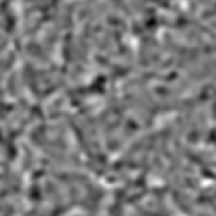
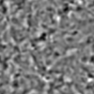
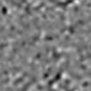
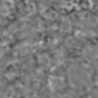
Fig. 1 shows a numerical illustration of this cross-correlation. The similarities between the left and the right maps are not striking. Yet, under close examination one can recognize individual patterns shared between the maps. Moreover, computation of correlation coefficient gives significant overlapping up to 40%.

Using this results, we define two quantities insensitive to the normalization of CMB and $\sigma_{8}$ and to filtering effects, which probe the cross-correlation between two lensing planes:

$${\cal X}_{{\Delta}}\equiv\frac{\left\langle\Delta\hat{B}\,b_{{\Delta}}(\vec{\alpha})\right\rangle}{\left\langle\Delta\hat{E}^{2}\right\rangle\left\langle\kappa_{\mathrm{{gal}}}^{2}\right\rangle}=-\frac{\left\langle\kappa\kappa_{\mathrm{{gal}}}\right\rangle}{\left\langle\kappa_{\mathrm{{gal}}}^{2}\right\rangle},\quad{\cal X}_{{\nabla}}\equiv\frac{\left\langle\Delta\hat{B}\,b_{{\nabla}}(\vec{\alpha})\right\rangle}{\left\langle(\vec{\nabla}\hat{E})^{2}\right\rangle\left\langle(\vec{\nabla}\kappa_{\mathrm{{gal}}})^{2}\right\rangle}=-\frac{1}{2}\frac{\left\langle\vec{\nabla}\kappa\cdot\vec{\nabla}\kappa_{\mathrm{{gal}}}\right\rangle}{\left\langle\vec{\nabla}\kappa_{\mathrm{{gal}}}^{2}\right\rangle}$$ (6)

Previous methods to probe weak lensing in CMB anisotropies $\!{}^{{\bf?},{\bf?}}$ ran into high cosmic variance problems. This is not surprising since lens effect which is not dominant can be masked by statistical deviations of the primary CMB signal, thus reducing the accuracy of lens detection. Since $B$ polarization only emerges in presence of lensing, this last effect should be less important. Indeed, we showed in $\!{}^{{\bf?}}$ that ${\cal X}_{{\Delta}}$ cosmic variance can be simply estimated in terms of the cosmic variances of the polarization field and of the shear field.

$${\mathrm{C}osVar}({\cal X}_{{\Delta}})={\mathrm{C}osVar}\left(\left\langle\Delta E^{2}\right\rangle\right)+\left(\frac{1+r^{2}}{2\,r^{2}}\right){\mathrm{C}osVar}\left(\left\langle\kappa^{2}\right\rangle\right).$$ (7)

The same kind of equation holds for ${\cal X}_{{\nabla}}$. This expression leads to values for the cosmic variance of ${\cal X}_{{\Delta}}$ of less than 8% for realistic 100 square degrees surveys (see table 1).

Table 1: Values of the cosmic variance of ${\cal X}_{\natural}$. The survey size is $100\,\textrm{deg}^{2}$. We used the results of ray-tracing simulation from $\!{}^{{\bf?}}$ and the $C_{l}$ given by “CMBSlow”$\!{}^{{\bf?}}$. From this estimations, we can expect a cosmic variance for ${\cal X}_{\natural}$of less than 10% for realistic scenarii.

	${\mathrm{C}osVar}\left({\cal X}_{{\Delta}}\right)$		${\mathrm{C}osVar}\left({\cal X}_{{\nabla}}\right)$
	$\Omega_{0}=0.3$	$\Omega_{0}=1$	$\Omega_{0}=0.3$	$\Omega_{0}=1$
$\theta=5^{\prime},\,\theta_{\mathrm{{gal}}}=2.5^{\prime}$	6.44%	4.77%	6.06%	4.72%
$\theta=5^{\prime},\,\theta_{\mathrm{{gal}}}=5^{\prime}$	6.58%	4.79%	4.99%	4.23%
$\theta=10^{\prime},\,\theta_{\mathrm{{gal}}}=5^{\prime}$	8.71%	6.73%	9.49%	7.62%

4 Conclusion - Sensitivity to the cosmic parameters

We showed that weak lensing effect on the CMB $B$ polarization can be embedded in a simple, real space, first order expression. This expression can be used to create mathematical objects that compare the lensing effects up to the last scattering surface to the one up to our galaxy surveys probes. We showed that this objects should produce a significant information, even in realistic (i.e. filtered) situations, with a low intrinsic statistical error.

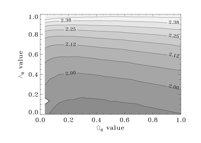
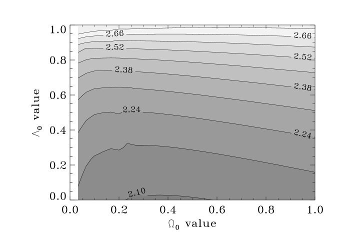
These objects are also expected to be good, unbiased, cosmic parameters tracers. Fig. 2 presents their behavior in the $(\Omega_{0},\Lambda)$ plane which exhibit a high sensitivity to the vacuum energy density. This is not surprising, since we are probing the length of the optical bench we are working in, which is rather sensitive to $\Lambda$ $\!{}^{{\bf?},{\bf?}}$.

Figure 2: ${\cal X}_{{\Delta}}$ (left figure) and ${\cal X}_{{\nabla}}$ for a CDM model. The filtering beam is 2 arc minutes for all fields.

References

- [1] K. Benabed, F. Bernardeau & L. van Waerbeke, astro-ph/0003038
- [2] Y. Mellier, ARAA 37 (1999) 127.
- [3] A. Blanchard, J. Schneider A&A 184 (1987) 1 ; U. Seljak ApJ 463 (1996) 1 .
- [4] F. Bernardeau, A&A 324 (1997) 15 ; M. Zaldarriaga, astro-ph/9910498 ; F. Bernardeau, A&A 338 (1998) 767 ; U. Seljak, M. Zaldarriaga, Phys.Rev.Lett. 82 (1999) 2636; M. Zaldarriaga, U. Seljak, Phys.Rev. D; J. Guzik, U. Seljak & M. Zaldarriaga, astro-ph/9912505.
- [5] M. Zaldarriaga, U. Seljak, Phys.Rev. D58 (1998) 023003 ; K. Benabed & F. Bernardeau, astro-ph/9906161, Phys. Rev D, in press; W. Hu, astro-ph/0001303.
- [6] M. Suginohara, T. Suginohara, D. N. Spergel, ApJ 495 (1998) 511 ; H. V. Peiris & D. N. Spergel, astro-ph/0001393 ; L. Van Waerbeke, F. Bernardeau & K. Benabed, astro-ph/9910366.
- [7] V. Faraoni, Astron.Astrophys. 272 (1993) 385.
- [8] F. Bernardeau, L. Van Waerbeke, Y. Mellier Astronomy and Astrophysics, 322 (1997) 1.
- [9] U. Seljak, ApJ 482 (1997) 6; W. Hu & M. White, New Astronomy 2 (1997) 323; J. Lesgourgues, D. Polarski, S. Prunet, A. A. Starobinsky gr-qc/9906098.
- [10] A. Riazuelo, PhD thesis, University of Paris 11.
- [11] B. Jain, U. Seljak, S. White, To appear in ApJ, astro-ph/9901191.