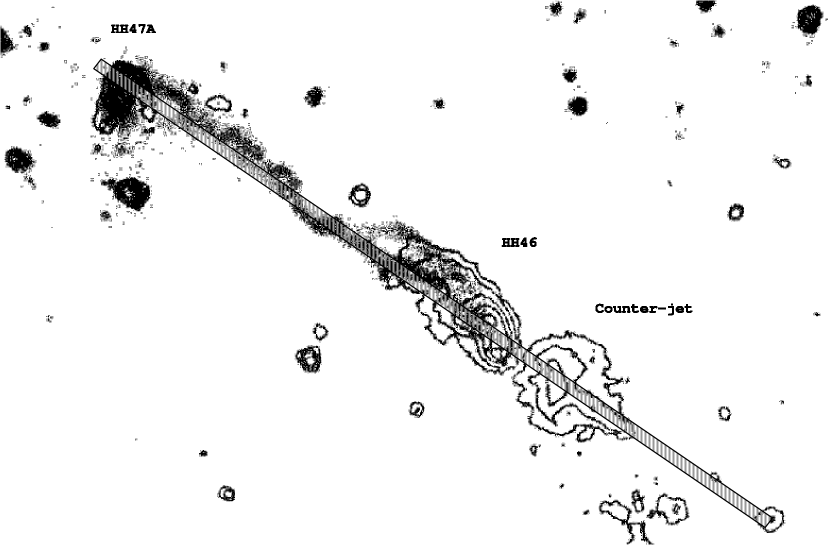
Figure 1: Image of the region studied in the HH46/47 complex. The observed slit position is shown superposed on a [SII] 0.673 m plus H2 1-0 S(1) 2.12 m (contours) map. Adapted from Eislöffel et al. (1994).
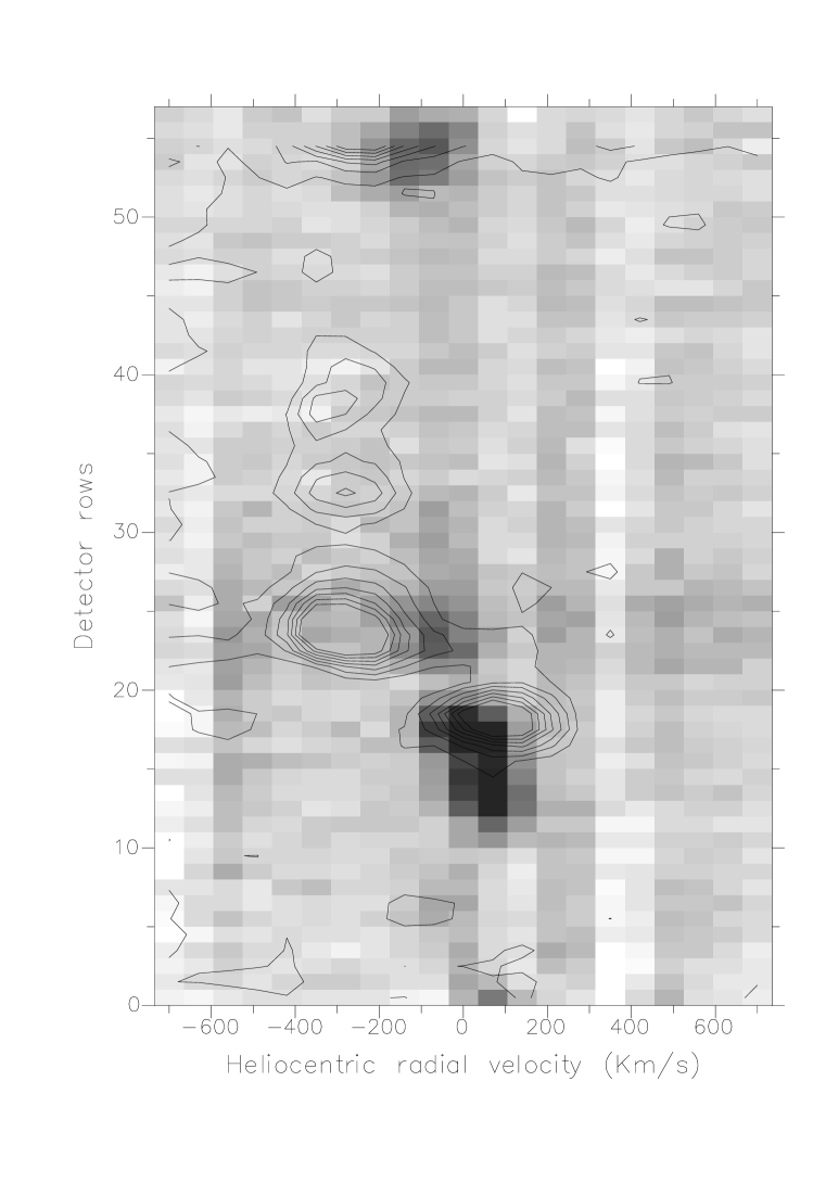
Figure 2: Near-infrared contour emission map obtained for the
H2 1-0 S(1) transition on the HH46/47 object. The position of the
HH objects are labelled in this figure, as well as the bright and
extended counter-jet flow. The spatial co-ordinate is given in
IRSPEC rows (each corresponding to a length of 2.2″ per pixel on the
sky) on the left axis. To plot this image, we used 7
contours increasing in steps of from a base level of
erg s-1cm-2 m-1. The vertical line is plotted at
zero heliocentric radial velocity.
Figure 3: Position-velocity emission maps obtained for the higher excitation
H2 line emission discussed in the main text. The 2-1S(1)
transition has contours plotted linearly from a base contour of
erg s-1cm-2 m-1, and stepped by erg s-1cm-2 m-1.
The 1-0S(0) transition has contours plotted linearly from a base
contour of erg s-1cm-2 m-1, and stepped by erg s-1cm-2 m-1. The 2-1S(2) transition has contours plotted linearly
from a base contour of erg s-1cm-2 m-1, and stepped by
erg s-1cm-2 m-1. The 3-2 S(3) transition
has contours plotted linearly from a base contour of erg s-1cm-2 m-1, and stepped by erg s-1cm-2 m-1.
Figure 4: H2 excitation diagrams for the
counter-jet. The derredened column
densities are plotted against the transition upper level
energy for the four H2 lines (labelled next to the plotted
data point) observed with the highest signal-to-noise (see
Table 3). The arrow in the plot
represents a 3 upper limit.
The solid line represents the least squares fit
to the errorless data
points providing an excitation temperature of
K ( 300 K) for the whole
counter-jet (Total; bottom diagram) and
the northern peak in
the counter-jet (North; top diagram)
Figure 5:
Position-velocity emission maps obtained in the [Fe ii] 1.257 m and
[Fe ii] 1.644 m transitions. For the [Fe ii] 1.644 m, the base contour is plotted at
erg s-1cm-2 m-1 with a linear step of erg s-1cm-2 m-1 whereas for the [Fe ii] 1.257 m, the base contour is at
erg s-1cm-2 m-1 and adjacent contours are stepped linearly
by erg s-1cm-2 m-1. In both maps, the vertical solid lines
are drawn at zero velocity emission whereas the horizontal solid
lines is drawn at the position of the continuum
emission from the HH46 object. These positions have been
calculated using the spatial offsets given in Table 1.
Figure 6: Spatial emission profiles of the observed slit.
Figure 7: Overlay of the H2 1-0 S(1) and [Fe ii] 1.644 m emission maps.