Clustering statistics on a light-cone in the cosmological redshift space

Abstract

We summarize a series of our recent work concerning the cosmological redshift-space distortion and light-cone effects. After briefly describing the theoretical formalism, we show how those effects are sensitive to the cosmological parameters. Then we apply this formalism to predict the two-point correlation functions and power spectra for the X-ray clusters, galaxies and quasars in future surveys, and discuss their cosmological implications.

1. Cosmological effects in the high-z universe

Redshift surveys of galaxies definitely serve as the central database for observational cosmology. In addition to the existing catalogues including CfA1, CfA2, SSRS, and the Las Campanas survey, upcoming galaxy surveys such as 2dF (2-degree Field Survey) and SDSS (Sloan Digital Sky Survey) are expected to provide important clues to the evolution of structure in the universe. In addition to those shallower surveys, clustering in the universe in the range $z=1-3$ has been partially revealed by, for instance, the Lyman-break galaxies and X-ray selected AGNs. In particular, the 2dF and SDSS QSO redshift surveys promise to extend the observable scale of the universe by an order of magnitude, up to a few Gpc. A proper interpretation of such redshift surveys in terms of the clustering evolution, however, requires an understanding of many cosmological effects which can be neglected for $z\ll 1$ and thus have not been considered seriously so far. These cosmological contaminations include linear redshift-space (velocity) distortion (Kaiser 1987), nonlinear redshift-space (velocity) distortion (e.g., Suto & Suginohara 1991; Cole, Fisher, & Weinberg 1994), cosmological redshift-space (geometrical) distortion (Alcock & Paczyński 1979; Ballinger, Peacock, & Heavens 1996; Matsubara & Suto 1996), and cosmological light-cone effect (Yamamoto & Suto 1999; Suto et al. 1999; Yamamoto, Nishioka & Suto 1999).

We describe a theoretical formalism to incorporate those effects, in particular the cosmological redshift-distortion and light-cone effects, and present several specific predictions in cold dark matter (CDM) models.

2. Cosmological redshift-space distortion

Due to a general-relativistic effect through the geometry of the universe, the observable separations perpendicular and parallel to the line-of-sight direction, $x_{{\rm s}{\scriptscriptstyle\perp}}=(c/H_{0})z\delta\theta$ and $x_{{\rm s}{\scriptscriptstyle\parallel}}=(c/H_{0})\delta z$, are mapped differently to the corresponding comoving separations in real space $x_{{\scriptscriptstyle\perp}}$ and $x_{{\scriptscriptstyle\parallel}}$:

$$x_{{\rm s}{\scriptscriptstyle\perp}}(z) = x_{\perp}cz/[H_{0}(1+z)d_{\rm\scriptscriptstyle{A}}(z)]\equiv x_{\perp}/c_{\perp}(z),$$ (1)

$$x_{{\rm s}{\scriptscriptstyle\parallel}}(z) = x_{\parallel}H(z)/H_{0}\equiv x_{\parallel}/c_{\parallel}(z),$$ (2)

with $d_{\rm\scriptscriptstyle{A}}(z)$ being the angular diameter distance. The difference between $c_{\perp}(z)$ and $c_{\parallel}(z)$ generates an apparent anisotropy in the clustering statistics, which should be isotropic in the comoving space. Then the power spectrum in cosmological redshift space, $P^{({\rm\scriptscriptstyle{CRD}})}$, is related to $P^{({\rm S})}$ defined in the comoving redshift space as

$$P^{({\rm\scriptscriptstyle{CRD}})}(k_{{\rm s}\perp},k_{{\rm s}\parallel};z)=\frac{1}{c_{\perp}(z)^{2}c_{\parallel}(z)}P^{({\rm S})}\left(\frac{k_{{\rm s}{\scriptscriptstyle\perp}}}{c_{\perp}(z)},\frac{k_{{\rm s}{\scriptscriptstyle\parallel}}}{c_{\parallel}(z)};z\right),$$ (3)

where the first factor comes from the Jacobian of the volume element $dk_{{\rm s}{\scriptscriptstyle\perp}}^{2}dk_{{\rm s}{\scriptscriptstyle\parallel}}$, and $k_{{\rm s}\perp}=c_{\perp}(z)k_{\perp}$ and $k_{{\rm s}\parallel}=c_{\parallel}(z)k_{\parallel}$ are the wavenumber perpendicular and parallel to the line-of-sight direction. If one assumes a scale-independent deterministic linear bias, the power spectrum distorted by the peculiar velocity field, $P^{({\rm S})}(k;z)$, is known to be well approximated by the following expression (Cole et al. 1995; Peacock & Dodds 1996):

$$P^{({\rm S})}(k_{\perp},k_{\parallel};z)=b^{2}(z)P^{({\rm R})}_{{\rm\scriptscriptstyle mass}}(k;z)\left[1+\beta(z)\left(\frac{k_{\parallel}}{k}\right)^{2}\right]^{2}D\left[k_{\parallel}{\hbox{$\sigma_{\scriptscriptstyle{\rm P}}$}}(z)\right],$$ (4)

where $k_{\perp}$ and $k_{\parallel}$ are the comoving wavenumber perpendicular and parallel to the line-of-sight of an observer, and $P^{({\rm R})}_{{\rm\scriptscriptstyle mass}}(k;z)$ is the mass power spectrum in real space. The finger-of-god effect is modeled by the damping function, $D\left[k_{\parallel}{\hbox{$\sigma_{\scriptscriptstyle{\rm P}}$}}(z)\right]$, for which we assume a Lorentzian. Then equation (3) reduces to

$$P^{({\rm\scriptscriptstyle{CRD}})}(k_{\rm s},\mu_{k};z) = \frac{b^{2}(z)}{c_{\perp}(z)^{2}c_{\parallel}(z)}P^{({\rm R})}_{\rm\scriptscriptstyle mass}\left(\frac{k_{\rm s}}{c_{\perp}(z)}\sqrt{1+\left[{1\over\eta(z)^{2}}-1\right]\mu_{k}^{2}};z\right)$$ (6)

$$\times\left\{1+\left[{1\over\eta(z)^{2}}-1\right]\mu_{k}^{2}\right\}^{-2}\left\{1+\left[{1+\beta(z)\over\eta(z)^{2}}-1\right]\mu_{k}^{2}\right\}^{2}~{}\left[1+\frac{k_{\rm s}^{2}\mu_{k}^{2}{\hbox{$\sigma_{\scriptscriptstyle{\rm P}}$}}^{2}}{2c^{2}_{\parallel}(z)}\right]^{-1},$$

where we introduce

$$k_{\rm s}\equiv\sqrt{k_{{\rm s}\perp}^{2}+k_{{\rm s}\parallel}^{2}},\quad\mu_{k}\equiv k_{{\rm s}\parallel}/k_{\rm s},\quad\eta\equiv c_{\parallel}/c_{\perp},$$ (7)

following Ballinger et al. (1996) and Magira et al. (2000).

Fig. 1.: Two-dimensional power spectra in cosmological redshift space at $z=2.2$.

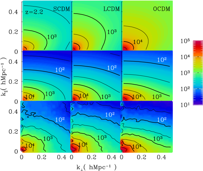
Figure 1. shows anisotropic power spectra $P^{({\rm\scriptscriptstyle{CRD}})}(k_{\rm s},\mu_{k};z=2.2)$. As specific examples, we consider SCDM (standard CDM), LCDM (Lambda CDM), and OCDM (Open CDM) models, which have $(\Omega_{0},\lambda_{0},h,\sigma_{8})$ $=(1.0,0.0,0.5,0.6)$, $(0.3,0.7,0.7,1.0)$, and $(0.3,0.0,0.7,1.0)$, respectively. These sets of cosmological parameters are chosen so as to reproduce the observed cluster abundance (Kitayama & Suto 1997). Our theoretical predictions use the fitting formulae of Peacock & Dodds (1996; PD) for the nonlinear power spectrum, $P^{({\rm R})}_{{\rm\scriptscriptstyle{mass}}}(k;z)=2\pi^{2}\Delta^{2}_{\rm\scriptscriptstyle NL}(k,z)/k^{3}$, of Mo, Jing, & Börner (1997) for the pair-wise peculiar velocity dispersions:

$$\sigma_{\scriptscriptstyle{\rm\scriptscriptstyle P,MJB}}^{2} \equiv \Omega(z)H_{0}^{2}\left[1-\frac{1+z}{D_{+}^{2}(z)}\int_{z}^{\infty}\frac{D_{+}^{2}(z^{\prime})}{(1+z^{\prime})^{2}}dz^{\prime}\right]\int_{0}^{\infty}\frac{dk}{k}\frac{\Delta^{2}_{\rm\scriptscriptstyle NL}(k,z)}{k^{2}},$$ (8)

with $D_{+}(z)$ being the linear growth rate. Clearly the linear theory predictions ($\sigma_{\scriptscriptstyle{\rm P}}=0$; top panels) are quite different from the results of N-body simulations (bottom panels), indicating the importance of the nonlinear velocity effects ($\sigma_{\scriptscriptstyle{\rm P}}=\sigma_{\scriptscriptstyle{\rm\scriptscriptstyle P,MJB}}$; middle panels).

Fig. 2.: The confidence contours on $\Omega_{0}$-$\lambda_{0}$ plane from the $\chi^{2}$-analysis of the monopole and quadrupole moments of the power spectrum in the cosmological redshift space at $z=2.2$. We randomly selected $N=5\times 10^{3}$ (upper panels), $N=5\times 10^{4}$ (middle panels), and $N=5\times 10^{5}$ (lower panels) particles from N-body simulation. The value of $\sigma_{8}$ is adopted from the cluster abundance.

Next we decompose the power spectrum into harmonics:

$$P(k,\mu_{k};z)=\sum_{l:{\rm even}}P_{l}(k)L_{l}(\mu_{k}),\quad P_{l}(k;z)\equiv\frac{2l+1}{2}\int^{1}_{-1}d\mu_{k}P(k,\mu_{k};z)L_{l}(\mu_{k}),$$ (9)

where $L_{l}(\mu_{k})$ are the $l$-th order Legendre polynomials. Similarly, the two-point correlation function is decomposed as

$$\xi(x,\mu_{x};z)=\sum_{l:{\rm even}}\xi_{l}(x)L_{l}(\mu_{x}),\quad\xi_{l}(x;z)\equiv\frac{2l+1}{2}\int^{1}_{-1}d\mu_{x}\xi(x,\mu_{x};z)L_{l}(\mu_{x}),$$ (10)

using the direction cosine, $\mu_{x}$, between the separation vector and the line-of-sight. The above multipole moments satisfy the following relations:

$$\xi_{l}(x;z)={1\over 2\pi^{2}i^{l}}\int_{0}^{\infty}P_{l}(k;z)j_{l}(kx)k^{2}dk,$$ (11)

with $j_{l}(kx)$ being spherical Bessel functions. Substituting $P^{({\rm\scriptscriptstyle{CRD}})}(k_{\rm s},\mu_{k};z)$ in equation (9) yields $P^{({\rm\scriptscriptstyle{CRD}})}_{l}(k_{\rm s};z)$, and then $\xi^{({\rm\scriptscriptstyle{CRD}})}({\bf x_{s}};z)$ can be computed from equation (11).

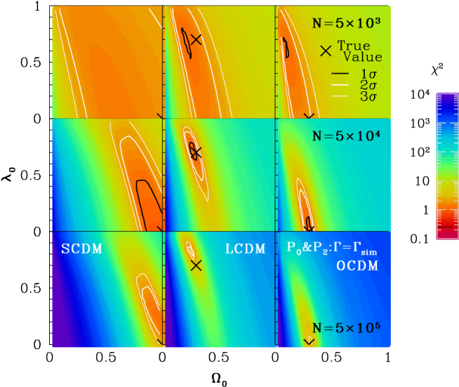
Comparison of the monopoles and quadrupoles from simulations and model predictions exhibits how the results are sensitive to the cosmological parameters, which in turn may put potentially useful constraints on $(\Omega_{0},\lambda_{0})$. Figure 2. indicates the feasibility, which interestingly results in a constraint fairly orthogonal to that from the Supernovae Ia Hubble diagram.

3. Cosmological light-cone effect

Observing a distant patch of the universe is equivalent to observing the past. Due to the finite light velocity, a line-of-sight direction of a redshift survey is along the time, as well as spatial, coordinate axis. Therefore the entire sample does not consist of objects on a constant-time hypersurface, but rather on a light-cone, i.e., a null hypersurface defined by observers at $z=0$. This implies that many properties of the objects change across the depth of the survey volume, including the mean density, the amplitude of spatial clustering of dark matter, the bias of luminous objects with respect to mass, and the intrinsic evolution of the absolute magnitude and spectral energy distribution. These aspects should be properly taken into account in order to extract cosmological information from observed samples of redshift surveys. We apply the formulation on the light-cone originally developed by Yamamoto & Suto (1999) to X-ray selected clusters and on-going SDSS galaxy and QSO catalogues.

3.1. Two-point correlation functions of X-ray selected clusters

Provided an X-ray flux-limited sample of clusters ($S>S_{\rm lim}$), it is fairly straightforward to compute its two-point correlation function $\xi^{\rm S}_{\rm cl}(R,z;>S_{\rm lim})$ at a given $z$; a fairly accurate empirical expression for the bias parameter $b(z)$ as a function of the halo mass is known (e.g., Jing 1998), and the mass is translated to the X-ray temperature assuming the virial equilibrium, and then to the X-ray luminosity from the observed luminosity-temperature relation (e.g., Kitayama & Suto 1996). The corresponding correlation function on the light-cone is given by

Fig. 3.: Light-cone and redshift-space distortion effects on two-point correlation functions of clusters.

$$\xi^{\rm LC}_{\rm X-cl}(R;>S_{\rm lim})={{\displaystyle\int_{z_{\rm min}}^{z_{\rm max}}dz{dV_{\rm c}\over dz}~{}n_{0}^{2}(z)\xi^{\rm S}_{\rm cl}(R,z(r);>S_{\rm lim})}\over{\displaystyle\int_{z_{\rm min}}^{z_{\rm max}}dz{dV_{\rm c}\over dz}~{}n_{0}^{2}(z)}},$$ (12)

where $R$ is the comoving separation of a pair of clusters, $z_{\rm max}$ and $z_{\rm min}$ denote the redshift range of the survey, and $dV_{\rm c}/dz$ is the comoving volume element per unit solid angle (Suto et al. 2000; Moscardini et al. 2000). The comoving number density of clusters in the flux-limited survey, $n_{0}(z;>S_{\rm lim})$, is computed by integrating the Press – Schechter mass function.

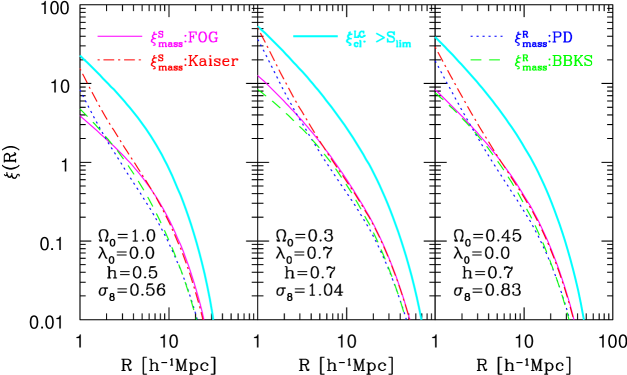
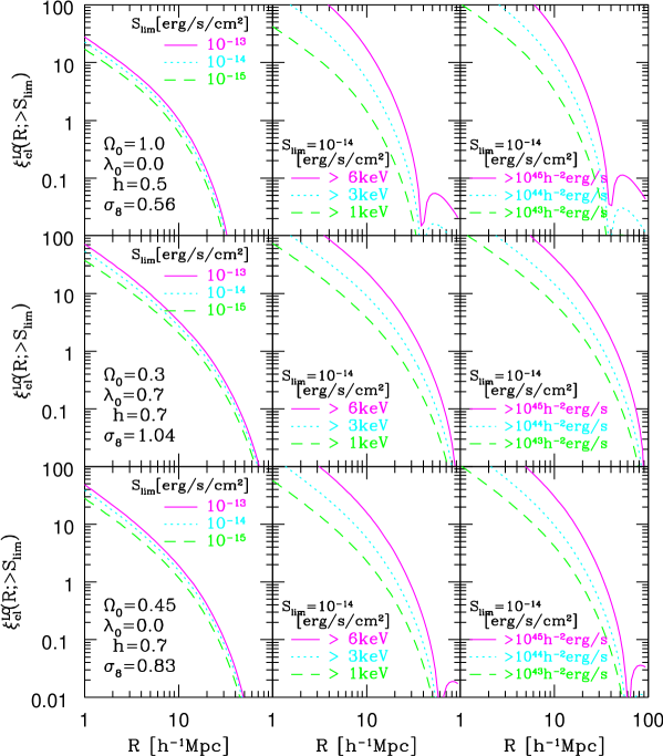
Figure 3. plots several predictions for two-point correlation functions under different assumptions; linear and nonlinear mass correlations in real space at $z=0$ using the Bardeen et al. (1986; BBKS) and PD formulae for mass power spectra, cluster correlations with linear redshift-space distortion (Kaiser 1987) and with full redshift-space distortion at $z=0$ using $\sigma_{\scriptscriptstyle{\rm\scriptscriptstyle P,MJB}}$. These should be compared with our final predictions on the light-cone in redshift space (with $S_{\rm lim}=10^{-14}$erg/s/cm²; thick solid lines). Figure 4. shows our predictions for $\xi^{\rm LC}_{\ cl}(R)$ for cluster samples selected with different flux-limit $S_{\rm lim}$ (left panels), and with additional temperature and absolute bolometric luminosity limits, $T_{\rm lim}$ and $L_{\rm lim}$ (middle and right panels). For the latter two cases, $S_{\rm lim}=10^{-14}$erg/s/cm² is assumed for definiteness. The results are insensitive to $S_{\rm lim}$, but very sensitive to $T_{\rm lim}$ and $L_{\rm lim}$, reflecting the strong dependence of the bias on the latter quantities.

Fig. 4.: Two-point correlation functions of clusters in SCDM (Top panels), LCDM (Middle panels), and OCDM (Bottom panels) for different selection criteria.

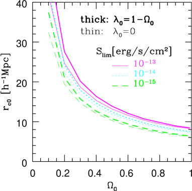
For a cosmological application of the present result, it is interesting to examine how $r_{c,0}(S_{\rm lim})$ defined through

$$\xi^{\rm LC}_{\rm cl}(r_{c0};>S_{\rm lim})=1$$ (13)

depends on $\Omega_{0}$. This is summarized in Figure 5., where we fix the value of the fluctuation amplitude $\sigma_{8}$ adopting the cluster abundance constraint (Kitayama & Suto 1997). Again the results are not sensitive to the flux limit $S_{\rm lim}$. The dependence on $\Omega_{0}$ is rather strong, and these predictions combined with the future observational results will be able to break the degeneracy of the cosmological parameters.

Fig. 5.: Correlation lengths of clusters as a function of $\Omega_{0}$. The shape parameter of the spectrum $\Gamma$ is fixed as $\Omega_{0}h\exp[-\Omega_{\rm b}(1+\sqrt{2h}\Omega_{0}^{-1})]$ with $\Omega_{\rm b}h^{2}=0.015$ and $h=0.7$.

3.2. Power spectra of SDSS galaxy and QSO samples

Finally we present theoretical predictions of power spectra relevant for SDSS galaxy and QSO samples, fully taking account of the cosmological redshift-space distortion and light-cone effects. Denoting the comoving number density and the selection function of the objects by $n_{0}^{{\rm\scriptscriptstyle{com}}}(z)$, and $\phi(z)$, Suto, Magira & Yamamoto (2000) obtain

$$P^{({\rm\scriptscriptstyle{LC}},{\rm\scriptscriptstyle{CRD}})}_{l}(k_{\rm s}) = {{\displaystyle\int_{z_{\rm min}}^{z_{\rm max}}dz{dV_{\rm c}\over dz}~{}[\phi(z)n_{0}^{{\rm\scriptscriptstyle{com}}}(z)]^{2}{c_{\perp}(z)^{2}c_{\parallel}(z)}P_{l}^{({\rm\scriptscriptstyle{CRD}})}(k_{\rm s};z)}\over{\displaystyle\int_{z_{\rm min}}^{z_{\rm max}}dz{dV_{\rm c}\over dz}~{}[\phi(z)n_{0}^{{\rm\scriptscriptstyle{com}}}(z)]^{2}{c_{\perp}(z)^{2}c_{\parallel}(z)}}}.$$ (14)

Figure 6. compares several predictions for the angle-averaged (monopole) power spectra normalized by the real-space counterpart in linear theory. The upper and lower panels adopt the selection functions appropriate for galaxies in $0<z<{z_{\rm max}}=0.2$ and QSOs in $0<z<{z_{\rm max}}=5$, respectively. The left and right panels present the results in SCDM and LCDM models. For simplicity we adopt a scale-independent linear bias model of Fry (1996),

$$b(z)=1+{1\over D_{+}(z)}[b(k,z=0)-1],$$ (15)

with $b(k,z=0)=1$ and $1.5$ for galaxies and quasars, respectively. It is clear that the cosmological redshift-space distortion and the light-cone effect substantially change the predicted shape and amplitude of the power spectra, even for the SDSS galaxy sample.

Fig. 6.: Light-cone and cosmological redshift-space distortion effects on angle-averaged power spectra.

4. Summary and conclusions

We have presented a theoretical formalism to predict the two-point clustering statistics on a light-cone in the cosmological redshift space. The present methodology will find two completely different applications. For relatively shallower catalogues like galaxy samples, the evolution of bias is not supposed to be so strong. Thus, one may estimate the cosmological parameters from the observed degree of the redshift distortion, as has been conducted conventionally. Most importantly, one can now correct for the systematics due to the light-cone and geometrical distortion effects, which affect the estimate of the parameters by $\sim 10$%. Alternatively, for deeper catalogues like high-redshift quasar samples, one can extract information on the nonlinearity, scale-dependence and stochasticity of the object-dependent bias only by correcting the observed data on the basis of our formulae. In this case, although one should adopt a set of cosmological parameters a priori, those will be provided both from the low-redshift analysis described above and from precision data of the cosmic microwave background and supernovae Ia. In a sense, the former approach uses the light-cone and geometrical distortion effects as real cosmological signals, while the latter regards them as inevitable, but physically removable, noise. In both cases, the present methodology is essential in properly interpreting the observations of the universe at high redshifts.

I thank Y.P.Jing, Tetsu Kitayama, Hiromitsu Magira, Takahiko Matsubara, Hiroaki Nishioka, and Kazuhiro Yamamoto for enjoyable collaborations on which the present talk is based. Numerical computations were carried out on VPP300/16R and VX/4R at the Astronomical Data Analysis Center of the National Astronomical Observatory, Japan, as well as at RESCEU and KEK (National Laboratory for High Energy Physics, Japan). This research was supported in part by the Grants-in-Aid by the Ministry of Education, Science, Sports and Culture of Japan to RESCEU (07CE2002).

References

1.   Alcock C., Paczyński B. 1979, Nature 281, 358

2.  Ballinger W.E., Peacock J.A., Heavens A.F. 1996, MNRAS 282, 877

3.  Bardeen J.M., Bond J.R., Kaiser N., Szalay A.S. 1986, ApJ 304, 15

4.   Cole S., Fisher K.B., Weinberg D.H. 1994, MNRAS 267, 785

5.   Fry J.N. 1996, ApJ 461, L65

6.   Jing Y.P. 1998, ApJ 503, L9

7.   Kaiser N. 1987, MNRAS 227, 1

8.   Kitayama T., Suto Y. 1996, ApJ 469, 480

9.   Kitayama T., Suto Y. 1997, ApJ 490, 557

10.  Magira H., Jing Y.P., Suto Y. 2000, ApJ 528, 30

11.  Matsubara T., Suto Y. 1996, ApJ 470, L1

12.  Mo H.J., Jing Y.P., Börner G. 1997, MNRAS 286, 979

13. Moscardini, L., Matarrese, S., Lucchin, F., & Rosati, P. 2000; MNRAS, submitted (astro-ph/9909273);

14.  Peacock J.A., Dodds S.J. 1996, MNRAS 280, L19

15.  Suto Y., Magira H., Jing Y.P., Matsubara T., Yamamoto K. 1999, Prog. Theor. Phys. Suppl. 133, 183

16. Suto Y., Magira H., Yamamoto K. 2000, PASJ, 52, No.2, in press

17. Suto Y., Suginohara T. 1991, ApJ 370, L15

18. Suto Y., Yamamoto K., Kitayama T., Jing Y.P. 2000, ApJ 534, May 10 issue, in press

19. Yamamoto K., Nishioka H., Suto Y. 1999, ApJ 527, 488

20. Yamamoto K., Suto Y. 1999, ApJ 517, 1