Depletion curves in cluster lenses: simulations and application to the cluster MS1008–1224

Abstract

When the logarithmic slope of the galaxy counts is lower than 0.4 (this is the case in all filters at large magnitude), the magnification bias due to the lens makes the number density of objects decrease, and consequently, the radial distribution shows a typical depletion curve. In this paper, we present simulations of depletion curves obtained in different filters for a variety of different lens models - e.g., a singular isothermal sphere, an isothermal sphere with a core, a power-law density profile, a singular isothermal ellipsoid and a NFW profile. The different model parameters give rise to different effects, and we show how the filters, model parameters and redshift distributions of the background populations affect the depletion curves. We then compare our simulations to deep VLT observations of the cluster MS1008–1224 and propose to constrain the mass profile of the cluster as well as the ellipticity and the orientation of the mass distribution. This application is based solely on deep photometry of the field and does not require the measurement of shape parameters of faint background galaxies. We finally give some possible applications of this method, useful for cluster lenses.

1 Introduction

Since a few years, a new application of gravitational lensing in clusters of galaxies has started to be explored, namely the depletion effect of number counts of background galaxies in cluster centers. This effect results from the competition between the gravitational magnification that increases the detection of individual objects (at least for flux limited data and marginally resolved objects) and the deviation of light beam that spatially magnifies the observed area and thus decreases the apparent number density of sources.

This effect was pointed out as a possible application of the magnification bias by Broadhurst et al. Broadhurst et al. (1995) where they suggested a new method for measuring the projected mass distribution of galaxy clusters, based solely on gravitational magnification of background populations by the cluster gravitational potential. In addition, they suggested that the mass-sheet degeneracy, initially pointed out by Schneider and Seitz Schneider and Seitz (1995) and observed in mass reconstruction with weak lensing measures, could be broken by using gravitational magnification information which is directly provided by the depletion curves. This method has been used by Fort et al. Fort et al. (1997) and by Taylor et al. Taylor et al. (1998) to reconstruct a two-dimensional mass map of Abell 1689 in the innermost 27 arcmin², taking into account the nonlinear clustering of the background population and shot noise. The results are consistent with those inferred from weak shear measurements and from strong lensing. However, the surface mass density cannot be obtained from magnification alone since magnification also depends on the shear caused by matter outside the data field Young (1981); Bartelmann and Schneider (2000). But in practice, if the data field is sufficiently large and no mass concentration lies close to but outside the data field, the mass reconstruction obtained from magnification can be quite accurate Schneider et al. (2000).

This method is an attractive alternative to weak lensing because it is only based on galaxy counts and does not require the measure of shape parameters of very faint galaxies. In addition, it is still valid in the intermediate lensing regime, close to the cluster center, without any strong modifications of the formalism. Meanwhile, it is more sensitive to Poisson noise which increases when the number density decreases in the depletion area. Another weak point identified by Schneider et al. Schneider et al. (2000) is that it may significantly depend on the galaxy clustering of background objects which can have large fluctuations from one cluster to another.

A second application of the magnification bias that has been suggested is to use the shape and the width of depletion curves to reveal the redshift distribution of the background populations. This technique was first used by Fort et al. Fort et al. (1997) in the cluster Cl0024+1654 to study the redshift distribution of background sources in the range $26<\mathrm{B}<28$ and $24<\mathrm{I}<26.5$. They found that $60\%\pm 10\%$ of the population in the B band is located between $z=0.9$ and $z=1.1$ while the remaining galaxies are broadly distributed around $z=3$. The population in the I band shows a similar redshift distribution but it extends to larger redshift $(\simeq 20\%$ of objects at $z>4)$.

The last application of the magnification bias that has been explored is the search for constraints on cosmological parameters. This method is based on the fact that the ratio of the two extreme radii which delimit the depletion area depends on the ratio of the angular distances lens-source and observer-source. Consequently it depends on the cosmological parameters, as soon as all the redshifts are fixed, and mainly on the cosmological constant. This method was first used by Fort et al. Fort et al. (1997) in Cl0024+1654 and in Abell 370. Their results favor a flat cosmology with $0.6<\Omega_{\Lambda}<0.85$ and are consistent with those obtained from other independent methods (see White White (1998)). This technique requires a good modeling of the lens and could be improved by being extended to a large number of cluster lenses and by using an independent estimate of the redshift distribution (for example from photometric redshifts). However, this method was disputed by Asada Asada (1997) who claimed that it is difficult to determine $\Omega$ by this method without the assumption of a spatially flat universe. He also mentioned the uncertainty of the lens model as one of the most serious problems in this test and concluded that this method cannot be taken as a clear cosmological test to determine $\Lambda$.

In order to better understand the formation of depletion curves and their dependence with the main characteristics of the lenses and the sources, we developed a detailed modeling of the curves in various conditions. In Sect. 2 we present the lens and counts models used in our simulations. In Sect. 3 we study the influence of the lens mass profile, with several sets of analytical mass distributions. In Sect. 4 we explore the influence of background sources distribution, selected through different filters. An application on real data is presented in Sect. 5, in the cluster MS 1008–1224, observed with the VLT. We compare these observations with the simulations in order to derive some constraints on the mass profile and the ellipticity of the cluster, as well as on the background sources distribution. Some prospects about the future of this method are given as a conclusion in Sect. 6.
Throughout the paper, we adopt a Hubble constant of H${}_{0}=50$ km s^-1 Mpc^-1, with $\Omega_{\Lambda}=0$ and $\Omega_{0}=1$.

2 Modeling depletion curves

2.1 The magnification bias

The projected number density of objects magnified by a factor $\mu$ through a lensing cluster and with magnitude smaller than $m$ can be written in the standard form:

$$\mathrm{N}(<m)=\mathrm{N}_{0}(<m)\ \mu^{2.5\gamma-1}$$

where $\mathrm{N}_{0}$ is the number density of objects in an empty field and $\gamma$ is the logarithmic slope of the galaxy number counts. Note first that this relation applies only for background galaxies. This means that we implicitly work at faint magnitude where the foreground counts are reduced and do not affect the slope $\gamma$. Note also that the magnification $\mu$ depends on the source redshift through the geometric factor $\mathrm{D}_{LS}/\mathrm{D}_{OS}$ in a significant way. For example, for $z_{L}=0.4$, $\mathrm{D}_{LS}/\mathrm{D}_{OS}$ changes by more than 40% when $z_{S}$ varies from 0.8 to 2. For a lower redshift cluster lens, the effect should be reduced, at least for all sources at $z>0.8$.

An exact writing of the magnification bias, which also takes into account the local effect of magnification, changing with radius $r$ within the lens can be re-formulated as:

$$\frac{\mathrm{N}(r,<m)}{\mathrm{N}_{0}(<m)}=$$ (1)

$$=\frac{\int_{0}^{z_{L}}n(z,<m)\ dz+\int_{z_{L}}^{+\infty}n(z,<m)\ \mu(r,z)^{2.5\gamma-1}\ dz}{\int_{0}^{+\infty}n(z,<m)\ dz}$$

$$=1-\frac{\int_{z_{L}}^{+\infty}n(z,<m)\left[1-\mu(r,z)^{2.5\gamma-1}\right]dz}{\mathrm{N}_{0}(<m)}$$

where $n(z,<m)$ is the density of galaxies of apparent magnitude smaller than $m$, located at redshift $z$. $\gamma(z)$ represents the shape of the luminosity function at redshift $z$ and we will assume in the following that $\gamma$ does not depends on redshift, i.e. most of the faint galaxies are representative of the power-law part of the luminosity function. In addition we suppose that the slope is a constant with redshift.

It is clear that the radial behavior of the ratio $\mathrm{N}(r,<m)/\mathrm{N}_{0}(<m)$ is strongly related to $\mu(r)$. It decreases from the center, up to a minimum at $r\sim R_{E}$ when magnification goes to infinity (Einstein radius) and then increases up to 1 again, when magnification goes to 0. This is the so-called radial depletion curve which has been detected in a few clusters already Fort et al. (1997); Taylor et al. (1998); Athreya et al. (2000).

From the lensing point of view, the magnification $\mu$ can be written as Schneider et al. (1992) :

$$\mu=\frac{1}{\mathrm{det}\mathcal{A}}=\frac{1}{(1-\kappa)^{2}-\gamma^{2}}$$ (2)

where $\mathcal{A}$ is the magnification matrix. The convergence $\kappa$ and the shear $\gamma$ are expressed in cartesian coordinates as a function of the reduced gravitational potential $\varphi$ by :

$$\kappa=\frac{1}{2}\left(\frac{\partial^{2}\varphi}{\partial x^{2}}+\frac{\partial^{2}\varphi}{\partial y^{2}}\right)$$ (3)

$$\gamma=\sqrt{\gamma_{1}^{2}+\gamma_{2}^{2}}$$ (4)

with :

$$\gamma_{1}=\frac{1}{2}\left(\frac{\partial^{2}\varphi}{\partial x^{2}}-\frac{\partial^{2}\varphi}{\partial y^{2}}\right)\quad{\mathrm{and}}\quad\gamma_{2}=\frac{\partial^{2}\varphi}{\partial x\partial y}$$

All these factors depend on the lens and source redshifts, as $\varphi$ is related to the true projected potential $\Phi$ by :

$$\varphi=\frac{2}{c^{2}}\ \frac{1}{\zeta^{2}}\ \frac{\mathrm{D}_{LS}\mathrm{D}_{OL}}{\mathrm{D}_{OS}}\ \Phi$$

where $\zeta$ is a characteristic scale of the lens.

In the weak lensing regime we have the approximation $\mu(r)\sim 1+2\kappa(r)$ Broadhurst et al. (1995). So the potential interest of the depletion curves is that they trace directly the convergence distribution, or equivalently the surface mass density distribution. In principle, they may allow an easy mass reconstruction of lenses in the weak regime. We will see below what are the main limitations of such curves, already explored by Athreya et al. Athreya et al. (2000).

2.2 The cluster lens

Different sets of models are used, with increasing complexity. In all cases we suppose that the lens redshift is 0.4, with reference to the cluster Cl0024+1654 studied by Fort et al. Fort et al. (1997). With the adopted cosmology this means that the scaling corresponds to 6.4 $h_{50}^{-1}$ kpc for 1″. For each model we will use an analytic expression and develop it to compute analytically the magnification and its dependence with redshift and radius. All the models are scaled in terms of the Einstein radius $R_{E}$.

2.2.1 The singular isothermal sphere (SIS)

This model is the simplest one which can describe a cluster of galaxies and is very useful for the analytical calculations of the gravitational magnification. However it has also some physical meanings:

• it corresponds to a solution of the Jeans equation and thus it can be written as a function of the observed velocity dispersion;

• in a non-collisionnal description of the collapse of a self-gravitating system, the violent relaxation, during which particles exchange energy with the average field, leads to an isothermal distribution Binney and Tremaine (1987).

But, this model is only valid inside certain limits due to the divergence of the central mass density and of the total mass to infinity. This divergence has no consequences on our work because the validity limits of the model correspond to the limits of the depletion regime. The density of matter can be written as :

$$\rho(r)=\rho_{E}\ \left(\frac{r}{R_{E}}\right)^{-2}$$ (5)

where $R_{E}$ is the Einstein radius :

$$R_{E}=4\pi\ \frac{\sigma^{2}}{c^{2}}\ \frac{D_{LS}D_{OL}}{D_{OS}}$$

and $\sigma$ is the velocity dispersion along the line of sight. The gravitational magnification is simply :

$$\mu^{-1}=1-\frac{R_{E}}{r}$$ (6)

2.2.2 The isothermal sphere with core radius

This model avoids the divergence of the mass density in the inner part of the cluster with an internal cut-off of the density distribution. We chose the following distribution, as described in Hinshaw and Krauss Hinshaw and Krauss (1987) or Grossman and Saha Grossman and Saha (1994). The density of matter is given by :

$$\rho(r)=\frac{3}{2\pi}\ \frac{\Phi_{0}}{GR_{C}^{2}}\ \frac{1+\frac{x^{2}}{3}\left|\Delta^{2}-1\right|}{(1+x^{2}\left|\Delta^{2}-1\right|)^{2}}$$ (7)

where $R_{C}$ is the core radius, $x=r/R_{E}$ and $\Phi_{0}$ is the central value of the gravitational potential.

In this case, the Einstein radius is $R_{E}=R_{C}\sqrt{\Delta^{2}-1}$, where :

$$\Delta=\frac{4\pi\sigma^{2}}{c^{2}}\ \frac{D_{LS}}{D_{OS}}\ \frac{D_{OL}}{R_{C}}$$

The magnification can be written as :

$$\mu^{-1}=\left[1-\Delta\left(1+x^{2}\left|\Delta^{2}-1\right|\right)^{-\frac{3}{2}}\right]\times$$ (8)

$$\qquad\qquad\left[1-\Delta\left(1+x^{2}\left|\Delta^{2}-1\right|\right)^{-\frac{1}{2}}\right]$$

Physically, in most cases the core radius is smaller than or comparable to the Einstein radius, so we do not expect strong effects in the outer parts of the depletion curves.

2.2.3 A power-law density profile

This model is a generalization of the SIS. It can be used in order to test the departure from an isothermal profile far away from the cluster center. The density is given by :

$$\rho=\rho_{E}\ \left(\frac{r}{R_{E}}\right)^{-\alpha}$$ (9)

where $\alpha$ is the logarithmic slope of the density profile. In order to keep a physical model for the mass distribution, we must have $\alpha<3$. The Einstein radius can be written as :

$$R_{E}=\sqrt{\frac{4}{c^{2}}\ \frac{D_{LS}D_{OL}}{D_{OS}}\ GM_{E}\ I_{\alpha/2}}$$

where $M_{E}=4\pi\rho_{E}R_{E}^{3}/\left(3-\alpha\right)$ is the integrated mass inside the Einstein radius and $I_{\beta}=\int_{0}^{+\infty}(1+\xi^{2})^{-\beta}\,d\xi$. The magnification is then :

$$\mu^{-1}=\left[1-(2-\alpha)\left(\frac{r}{R_{E}}\right)^{1-\alpha}\right]\times\left[1-\left(\frac{r}{R_{E}}\right)^{1-\alpha}\right]$$ (10)

2.2.4 The singular isothermal ellipsoid

This type of model is interesting as a lot of clusters have elliptical shapes in their galaxy distribution or their X-ray isophotes Buote and Canizares (1992, 1996); Lewis et al. (1999); Soucail et al. (2000). Thus, an elliptical lens represents a more realistic model although it is still reasonably simple. In order to study the effect of the ellipticity of the potential $\epsilon=1-\frac{b}{a}\;(a\geq b)$ on the depletion, we introduced the singular isothermal ellipsoid in our simulations Kormann et al. (1994). Using polar coordinates $(r,\varphi)$ in the lens plane we introduce

$$\zeta=\sqrt{\left(r\cos\varphi\right)^{2}+\left(1-\epsilon\right)^{2}\left(r\sin\varphi\right)^{2}}$$ (11)

which is constant on ellipses with minor axis $\zeta$ and major axis $\zeta/\left(1-\epsilon\right)$. The surface mass density can then be written as :

$$\Sigma\left(r,\varphi\right)=\frac{\sqrt{1-\epsilon}\>\sigma^{2}}{2G}\frac{1}{\zeta}$$ (12)

where $\sigma$ is the velocity dispersion along the line of sight.
The convergence is :

$$\kappa=\frac{\Sigma\left(r,\varphi\right)}{\Sigma_{critical}}=\Sigma\left(r,\varphi\right)\times\frac{4\pi G}{c^{2}}\ \frac{D_{OL}D_{LS}}{D_{OS}}$$ (13)

The magnification writes then quite simply:

$$\mu^{-1}=1-2\kappa$$ (14)

2.2.5 NFW profile

We introduced in our simulations the universal density profile of Navarro et al. Navarro et al. (1996) for dark matter halos which was found from cosmological simulations of the growth of massive structures. This profile is a very good description of the radial mass distribution inside the virial radius $r_{200}$. Wright and Brainerd Wright and Brainerd (2000) have compared it with a SIS for several cosmological models. They find that the assumption of an isothermal sphere potential results in an overestimate of the halos mass which increases linearly with the value of the NFW concentration parameter. This overestimate depends upon the cosmology and is smaller for rich clusters than for galaxy-sized halos.
The NFW density profile is given by :

$$\rho(r)=\frac{\delta_{c}\rho_{c}}{\left(r/r_{s}\right)\left(1+r/r_{s}\right)^{2}}$$ (15)

where $r_{s}=r_{200}/c$ is a characteristic radius and $\rho_{c}$ is the critical density. $c$ is the concentration parameter and $\delta_{c}$ is a characteristic over-density for the halo which is related to $c$ by the requirement that the mean density within the virial radius should be $200\rho_{c}$. This leads to :

$$\delta_{c}=\frac{200}{3}\frac{c^{3}}{\ln(1+c)-c/(1+c)}$$

If we take $x=r/r_{s}$, the surface mass density and the shear of a NFW lens can be written as Wright and Brainerd (2000):

$$\kappa_{\mathrm{NFW}}(x)=\frac{r_{s}\delta_{c}\rho_{c}}{\Sigma_{c}}\left\{\begin{array}[]{lr}f_{<}(x)&(x<1)\\ 2/3&\qquad(x=1)\\ f_{>}(x)&(x>1)\end{array}\right.$$

$$\gamma_{\mathrm{NFW}}(x)=\frac{r_{s}\delta_{c}\rho_{c}}{\Sigma_{c}}\left\{\begin{array}[]{lr}g_{<}(x)&(x<1)\\ 10/3+4\ln(1/2)&\quad(x=1)\\ g_{>}(x)&(x>1)\end{array}\right.$$

where $\Sigma_{c}$ is the critical surface mass density. $f_{<}(x)$ and $f_{>}(x)$ express as :

$$f_{<}(x)=\frac{2}{\left(x^{2}-1\right)}\left(1-\frac{2}{\sqrt{1-x^{2}}}\arg\mathrm{th}\sqrt{\frac{1-x}{1+x}}\,\right)$$

$$f_{>}(x)=\frac{2}{\left(x^{2}-1\right)}\left(1-\frac{2}{\sqrt{x^{2}-1}}\arctan\sqrt{\frac{x-1}{x+1}}\,\right)$$

while $g_{<}(x)$ and $g_{>}(x)$ express as :

$$g_{<}(x) = \frac{8\arg\mathrm{th}\sqrt{\frac{1-x}{1+x}}}{x^{2}\sqrt{1-x^{2}}}+\frac{4}{x^{2}}\ln\left(\frac{x}{2}\right)$$

$$\qquad-\frac{2}{\left(x^{2}-1\right)}+\frac{4\arg\mathrm{th}\sqrt{\frac{1-x}{1+x}}}{\left(x^{2}-1\right)\sqrt{1-x^{2}}}$$

$$g_{>}(x) = \frac{8\arctan\sqrt{\frac{x-1}{x+1}}}{x^{2}\sqrt{x^{2}-1}}+\frac{4}{x^{2}}\ln\left(\frac{x}{2}\right)$$

$$\qquad-\frac{2}{\left(x^{2}-1\right)}+\frac{4\arctan\sqrt{\frac{x-1}{x+1}}}{\left(x^{2}-1\right)^{\frac{3}{2}}}$$

The magnification by the NFW lens is then :

$$\mu^{-1}=\left(1-\kappa_{\mathrm{NFW}}\right)^{2}-\gamma_{\mathrm{NFW}}^{2}$$ (16)

2.3 The galaxy redshift distribution

2.3.1 Analytical distribution

We used the analytical redshift distribution introduced by Taylor et al. Taylor et al. (1998) to fit the redshift distribution of the galaxies in the range $20<I<24$ for $0.25<z<1.5$ :

$$N(z,I<24)=N_{0}(I<24)\frac{\alpha z^{2}}{z_{*}^{3}\Gamma(3/\alpha)}\exp\left[-\left(\frac{z}{z_{*}}\right)^{\alpha}\right]$$ (17)

with $\alpha=1.8$ and $z_{*}=0.78$. Here, we extend the redshift range between $z=0.05$ and $z=3$ and we take $N_{0}(I<24)=12$ objects per arcmin² which is the count rate found by Taylor et al. Taylor et al. (1998) for red galaxies with $20<I<24$. The distribution shows a maximum at $z=0.8$ and has an average redshift of $<z>\simeq 1$. It is worth noting that with these parameters, the redshift distribution does not correspond to very deep observations.

2.3.2 The magnitude-redshift distributions in the U to K photometric bands

We also used a model of galaxy number counts from which the magnitude-redshift distribution in empty field can be computed with a large set of photometric bands. This model was developed by Bézecourt et al. Bézecourt et al. (1998) and largely inspired by Pozetti et al. Pozetti et al. (1996). It includes the model of galaxy evolution developed by Bruzual and Charlot Bruzual and Charlot (1993), with the upgraded version so-called GISSEL, and standard parameters for the initial mass function (IMF) and star formation rates (SFR) for different galaxy types. In order to reproduce the deep number counts of galaxies, evolution of the number density of galaxies is included to compensate for the smaller volumes in an $\Omega_{0}=1$ universe, following the prescriptions of Rocca-Volmerange and Guiderdoni Rocca-Volmerange and Guiderdoni (1990). This model reproduces fairly well deep number counts up to $B=27$ or $I=25$, as well as redshift distributions of galaxies up to $B=24$ or $I=22$ Bézecourt et al. (1998).

Table 1: Magnitude ranges adopted for the field number counts in the simulations (see text for more details concerning the number count model).

Filter	Magnitude range	Faint end slope
B	22 – 28	0.14
I	20 – 26	0.23
K	18 – 23	0.22

The advantage of this model is that the galaxy distribution can be computed for any photometric band, and the effects of the color distribution of sources can be explored. In practice we will limit our study in this paper to B, I and K bands (Table 1).

3 Influence of the lens parameters on depletion curves

For our first set of simulations, we used the analytical redshift distribution for the sources, allowing a fully analytical treatment of the simulations. The contamination by foreground objects with this distribution is weak (about $\simeq 9\%$ of foreground galaxies for $z_{L}=0.4$). In each case, we computed depletion curves, and then examined their behavior. Note that we limited our analysis outside the first 20″ from the center where the signal cannot be constrained observationally (decrease in the observed area for each point, obscuration by the brightest cluster galaxies …). For these reasons, this “forbidden” area will be shaded in each plot.

3.1 Influence of the velocity dispersion

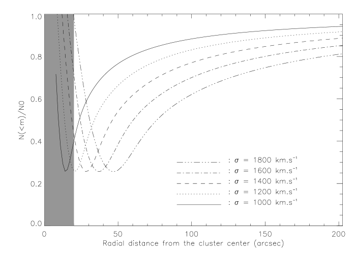
Figure 1: Top: Depletion curves obtained for different velocity dispersions ranging from 1000 to 1800 km s^-1. Bottom: Intensity of the minimum (solid line), position of the minimum in Mpc (dotted line) and half width at half minimum in Mpc (dashed line) of the depletion curves as a function of the velocity dispersion.

We used a SIS model and varied the velocity dispersion $\sigma$ from 1000 to 1800 km s^-1 (Fig. 1). As expected the radius of the minimum increases with $\sigma$. Indeed for a SIS, the Einstein radius scales exactly as $\sigma^{2}$, so the minimum of the depletion curve, which roughly corresponds to the maximum Einstein radius (at $z\sim 4$ or more), also scales as $\sigma^{2}$.

More surprisingly, the depth of the depletion at the position of the minimum is roughly constant and, at first order, does not depend on the velocity dispersion of the cluster or its total mass. Part of this effect is due to the density of foreground galaxies, but part of it is intrinsic to this SIS model, as other potential shapes do not show this property (see below). On the contrary there is a clear dependence on the half width at half minimum with $\sigma$ (Figure 1).

3.2 Influence of the core radius

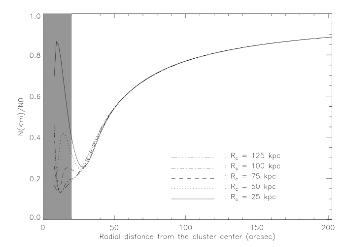
Figure 2: Depletion curves obtained with $\sigma=1400$ km s^-1 for different core radii ranging from 25 to 125 $h_{50}^{-1}$ kpc. The value of the Einstein radius at the cluster redshift is $\sim$ 200 $h_{50}^{-1}$ kpc.

The introduction of a core radius in the model (Fig. 2) does not affect significantly the outer region of the depletion area and has little effect on the position of the minimum. As $R_{C}$ increases, the inner width of the curve is enlarged and its slope is decreased. In fact, the study of this area for our purpose has no interest, because the spatial resolution of galaxy number counts variations is by far larger than this scale. In addition, in rich clusters of galaxies, the central density of galaxies is large enough so that empty areas are quite small between the envelopes of large and bright galaxies.

In practice, the only observable effect of a core radius is a deformation of the inner depletion curve with a significant departure from a symmetry with respect to the outer part. But we suspect that a quantitative estimate of $R_{C}$ would be difficult to extract from the signal.

3.3 Influence of the slope of the mass profile

Figure 3: Top: Depletion curves obtained with $\rho_{E}=2.25\times 10^{15}$ M${}_{\sun}/$Mpc³ and for different slopes $\alpha$ ranging from 1.7 to 2.1. Bottom: Intensity of the minimum (solid line), position of the minimum in Mpc (dotted line) and half width at half minimum in Mpc (dashed line) of the depletion curves as a function of the slope $\alpha$.

The simulations are done with the power-law density profile, characterised by its slope $\alpha$ (Fig. 3). The minimum position of the depletion area does not depend significantly of $\alpha$, because our scaling of the potential was fixed at the Einstein radius, nearly independent of $\alpha$. On the contrary, the two other typical features of the depletion area (half width at half minimum and intensity of the minimum) strongly depend on this parameter. The width of the curve represents roughly the mass dependence with radius. In the case $\alpha=1.7$ for example, the shallower slope of the mass radial dependence creates a larger width of the depletion curve. The half width at half minimum of the curve decreases when $\alpha$ increases. The reason is the same as with the SIS, that is to say, when $\alpha$ increases, the mass is concentrated in the inner part of the cluster and the depletion effect is less extended to the outer regions.

3.4 Influence of the ellipticity of the potential

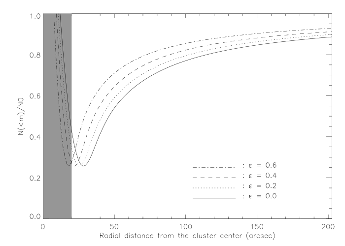
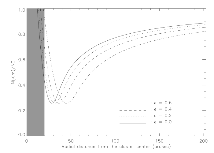
Figure 4: Top: Variation of the depletion curve with ellipticity along the minor axis. Bottom: Idem along the major axis. The streching of the curves with ellipticity is characterised by an homothetic transformation.

In these simulations, we use the singular isothermal ellipsoid potential, with $\sigma=1400$ km s^-1, and we study the depletion curves along the minor and major axis (Fig. 4). The increase of $\epsilon$ does not affect the minimum value of the depletion area but leads to an increase/decrease of the half width at half minimum and of the minimum position along the major/minor axis as an homothetic transformation. The relative positions of the two minima of the depletion area along the main axis gives immediately the axis ratio and thus the ellipticity of the potential. An application of this differential effect along the two main axis is presented in Sect. 5.

3.5 Study of NFW profile

Figure 5: Top: Depletion curves obtained with $c=15$ and for different virial radii. Bottom: Intensity of the minimum (solid line), position of the minimum in Mpc (dotted line) and half width at half minimum in Mpc (dashed line) of the depletion curves as a function of the virial radius.

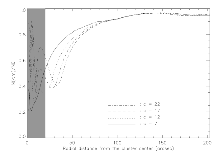
Figure 6: Top: Depletion curves obtained with $r_{200}=3000$ kpc and for different concentration parameters. Bottom: Intensity of the minimum (solid line), position of the minimum in Mpc (dotted line) and half width at half minimum in Mpc (dashed line) of the depletion curves as a function of the concentration parameter.

With the NFW model we varied separately the virial radius and the concentration parameter. We have chosen the values for these two parameters in the range of those found by Navarro et al. Navarro et al. (1996). For the first set of simulations, we adopted $c=15$ and varied $r_{200}$ from 1800 to 3600 kpc (Fig. 5). An increase of the virial radius (more massive cluster) leads to an increase of the three characteristic features of the depletion area and to the appearance of a bump in the central region which grows with $r_{200}$. The increase of the half width at half minimum of the depletion curves with $r_{200}$ can be explained by the fact that when $r_{200}$ increases there is more mass in the outer regions. Consequently, the depletion area is more extended to the outer part of the cluster and reaches its asymptotic value less rapidly. The second set of simulations was done with $r_{200}=3000$ kpc and we varied $c$ from 7 to 25 (Fig. 6). The variation of $c$ affects only the inner part of the depletion curves. An increase of the concentration parameter (cluster with smaller characteristic radius) leads to an increase of the intensity and position of the minimum with a steeper slope for the small values of $c$. Contrary to $r_{200}$, the variation of $c$ does not affect significantly the half width at half minimum of the depletion area.

4 Influence of background galaxies on depletion curves

In this section, we use a unique model for the lens, i.e. a SIS profile with a velocity dispersion of 1500 km s^-1 for a cluster located at $z_{L}=0.4$, to avoid effects due to the lens.

4.1 Effect of the lens on the magnitude-redshift distribution of background populations

Fig. 7 shows the distortion of the magnitude-redshift distribution in the B band along the curve. The results are qualitatively the same in the others bands. Near the cluster center, where the effects of the gravitational magnification are stronger, objects located just behind the lens show a gain in magnitude larger than 1. In the minimum area of the curve, the competition between gravitational magnification and dilatation is more favorable to high $z$ objects ($z>2.4$). In the outer part of the cluster, the effects of the gravitational magnification decrease and one finds again the distribution in empty field (asymptotic limit of the depletion curves).

Figure 7: Upper-left: Magnitude-redshift distribution of the galaxies in empty field computed from the model of Bézecourt et al. (1998), in the B-band; Upper-right: Depletion curve for $m_{Blim}=28$. The open squares show the points where the following $N_{lens}(m,z,r)$ distributions are computed. Middle-left: $r=31\arcsec$ (1); Middle-right: $r=42\arcsec$ (2); Lower-left: $r=70\arcsec$ (3); Lower-right: $r=125\arcsec$ (4).

4.2 Differential effects in several filters

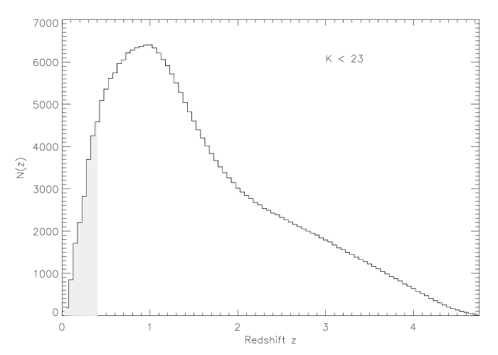
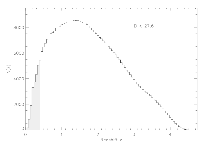
Figure 8: Depletion curves obtained in different filters for a SIS profile with $\sigma=1500$ km s^-1 (top left) and corresponding field redshift distributions for each filter and magnitude limit. The shaded area on the redshift distributions indicates the foreground contaminating population.

We first studied the evolution of the depletion area with the redshift distribution of the background population by considering several filters. We tried to determine some characteristics of the redshift distribution of background population which could be connected to typical features of the depletion area (Fig. 8). The magnitude limits of the simulations correspond to a typical observation time of about 2 hours on an 8-meter telescope with good imaging facilities. The contamination by foreground objects $(z<0.4)$ in the 3 filters is weak ($\simeq 8\%$ in the I and K bands and $\simeq 6\%$ in the B band for which the counts are deeper).
The evolution of the position of the minimum of the depletion area reflects the evolution of the mean redshift of the different populations ($<z>\simeq 1.57$ for the K band, $<z>\simeq 1.76$ for the B band and $<z>\simeq 1.79$ for the I band), but with a weak effect. The variation of the intensity of the minimum of the depletion area is connected for one part to the fraction of foreground objects and for the other part to the slope $\gamma$ of the luminosity function. As this slope decreases from I band to B band $(\gamma_{I}=0.23,\gamma_{K}=0.22,\gamma_{B}=0.14)$ with the magnitude thresholds we have chosen, the intensity of the minimum of the depletion area decreases in the same way from I band ($\simeq 0.31$) to B band ($\simeq 0.26$). Both features of the depletion curves are in fact weakly dependent on the choice of the filter and may be difficult to distinguish with real data, at least while the variation of the redshift distribution with wavelength is rather smooth.
On the contrary, the half width at half minimum of the depletion curve is affected by the redshift distribution of background populations in a more sensitive way. The increase of the half width at half minimum from B band to K band is anti-correlated with the fraction of objects at high redshift ($z>2$) for these populations which also decreases in the same way from B band ($\simeq 37\%$) to K band ($\simeq 29\%$) and seems to reflect essentially the bulk of galaxies at redshift around 1.

5 Depletion effect in the cluster MS1008–1224

We have applied our simulations to the cluster MS1008–1224 ($z=0.3062$, Lewis et al. Lewis et al. (1999)) which is one cluster of the Einstein Observatory Extended Medium Sensitivity Survey Gioia and Luppino (1994). It is a very rich galaxy cluster, slightly extended in X-rays, and it is also part of the Canadian Network for Observational Cosmology Survey Carlberg et al. (1996). Its galaxy distribution is quite circular, surrounding a North-South elongated core. There is a secondary clump of galaxies to the North. The X-ray luminosity is L_X(0.3-3.5 keV)$=4.5\times 10^{44}$ erg.s^-1 Gioia and Luppino (1994), the X-ray temperature inferred from ASCA observations is T${}_{X}=7.3$ keV Mushotzky and Scharf (1997) and the radio flux at 6 cm is lower than 0.8 mJy Gioia and Luppino (1994). Some gravitationally lensed arcs to the North and to the East of the field have been reported by Le Fèvre et al. Le Fèvre et al. (1994) as well as by Athreya et al. Athreya et al. (2000).

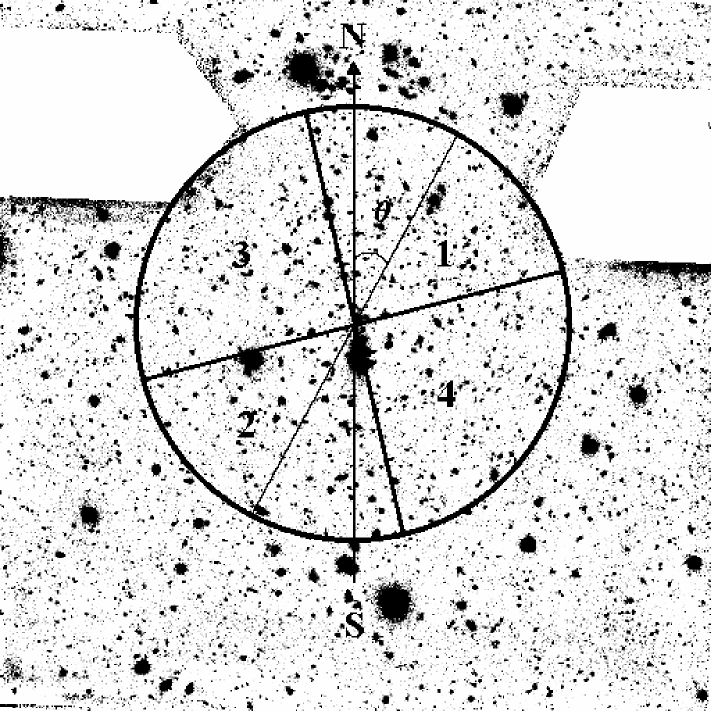
Figure 9: VLT FORS1 image of MS1008–1224 in the B band. North is up, East is left. The field-of-view is $6.8\arcmin\times 6.8\arcmin$. Note the two occulting masks hiding the brightest stars in the field.

Figure 10: Color-magnitude diagram R–I versus R of MS1008–1224. The two horizontal lines delimit the sequence of the cluster elliptical galaxies, which has been removed from our catalogue.

5.1 The observations

Data were obtained during very deep observations with FORS and ISAAC during the science verification phase of the VLT–ANTU (UT1) at Cerro Paranal (http://www.eso.org/science/ut1sv). Multicolor photometry was obtained in the B, V, R and I bands with FORS1 (field-of-view $6.8^{\prime}\times 6.8^{\prime}$) and in the J and Ks bands with ISAAC (field-of-view $2.5^{\prime}\times 2.5^{\prime}$) with sub-arcsecond seeing in all cases. The total exposure times are respectively 2880 seconds in J, 3600 seconds in Ks, 4050 seconds in I, 4950 seconds in B, 5400 seconds in V and R. We used the SExtractor software Bertin and Arnouts (1996) to construct our photometric catalogue. The completeness magnitudes are respectively $\mathrm{J}=24$, $\mathrm{Ks}=22$, $\mathrm{I}=25.5$, $\mathrm{V}=26.5$, $\mathrm{B}=26.5$ and $\mathrm{R}=26$. Our values are identical to those of Athreya et al. Athreya et al. (2000) concerning the FORS observations but they are one magnitude deeper concerning the ISAAC ones. In practice, we used only the FORS data which extend to a larger distance and are more suited to our study.

In order to remove part of the contamination by cluster members, we identified the elliptical galaxies by their position on the color–magnitude diagram (Fig. 10). So background sources were selected by removing this sequence, essentially valid at relatively bright magnitudes. This statistical correction is not fully reliable as it does not eliminate bluer cluster members or foreground sources. But it partly removes one cause of contamination, especially significant close to the cluster center. Our counts may also present an over-density of objects in the inner part of the cluster ($r<20\arcsec$) due to the non-correction of the surface of cluster elliptical galaxies we have removed, effect which is more sensitive in the inner part of the cluster where these galaxies are dominant. But as it is not in the most interesting region of the depletion area, we did not try to improve the measures there.

In addition, due to the presence of two 11 magnitude stars in the northern part of the FORS field, two occulting masks were put to avoid excessive bleeding and scattered light. We took into account this partial occultation of the observed surface for the radial counts above a distance of 130″ (see Fig. 9). This may possibly induce some additional errors in the last two points of the curves, which are probably underestimated, because of the difficulty to estimate the surface of the masks and some edge effects at the limit of the field.

5.2 Depletion curves and mass density profile

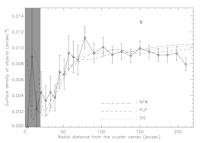
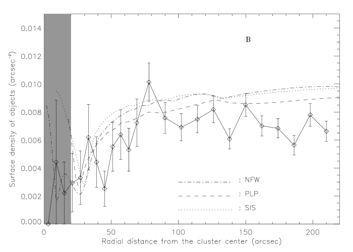
Figure 11: Depletion curves measured in MS1008–1224 in several spectral bands up to the completeness magnitude of the catalogues. For each plot, the best fit by the three models described in text are given. Error bars correspond to Poisson statistical noise. The shaded area on each plot corresponds to regions where the study of the depletion does not make sense (see text for more details).

The first step would be to locate the cluster center. Its position is rather difficult to estimate directly from the distribution of the number density of background sources, although in principle one should be able to identify it as the barycenter of the points with the lower density around the cluster. We did not attempt to fit it and preferred to fix it 15″ North of the cD, following both the X-ray center position Lewis et al. (1999) or the weak lensing center Athreya et al. (2000).

The radial counts were performed in a range of 3 magnitudes up to the completeness magnitude in the B, V, R and I bands and up to a radial distance of 210″ from the center, which covers the entire FORS field. The count step was fixed to 30 pixels (6″) in the innermost 80″ and for the rest of the field we adopted a count step of 60 pixels (12″) to reduce the statistical error bars. These values are a good balance between statistical errors in each bin which increase for small steps and a reasonable spatial resolution in the radial curve, limited by the bin size. The depletion curves obtained in the B, V, R and I bands are shown on Fig. 11. At some small limiting radius ($r<20\arcsec$), the ratio between the area of the count rings and the area covered by the cluster galaxies is close to unity. For this reason, we exclude the measures obtained in these innermost rings for any study of depletion effects (shaded regions on figure 11).

We fitted the observed depletion curve in the I-band with three of the mass models discussed above, namely a singular isothermal sphere, a power-law density profile and a NFW profile, and with the galaxy distribution described in §2.3.2. For each model, a $\chi^{2}$ minimization was introduced to derive the best fits and their related parameters (Table 2). The first fit included all the data points ($\chi^{2}_{\textrm{ap}}$) and gave poor results with a reduced $\chi^{2}$ always close to or larger than 2. A second fit was done after removing some clear deviant points ($\chi^{2}_{\textrm{wd}}$): the last two points probably poorly corrected from edge effects, and those associated to the overdensity seen at $r\simeq 80\arcsec$. This bump is easily identifiable in the V, R and I curves, and can be partly explained by the presence of a background cluster lensed by MS1008–1224 and identified by Athreya et al. Athreya et al. (2000). Nevertheless, even if we remove from our data all the lower right quadrant of the field where this structure is located, the bump is still there although significantly reduced. This suggests that it may be more extended behind the cluster center than initially suspected. This second fit gave more satisfying results. So we will consider the parameters associated with the best fit of each model as our best results.

• The velocity dispersion derived from the SIS model ($\sigma_{\textrm{fit}}=1200^{+200}_{-175}$ km s^-1) is in good agreement with the value measured by Carlberg et al. Carlberg et al. (1996) ($\sigma_{\textrm{obs}}=1054\pm 107$ km s^-1) but is more discordant with the value of 900 km s^-1 inferred from the shear analysis of Athreya et al. Athreya et al. (2000).

• The slope of the potential fit with a power-law density profile is close to an isothermal one ($\alpha=1.88$), although slightly shallower.

• For a NFW profile, we find a virial radius ($r_{200}=3.2h_{50}^{-1}$ Mpc) and a concentration parameter ($c=8.9$) quite in good agreement with those of Athreya et al. Athreya et al. (2000) derived from weak lensing measures.

• The comparison between the 3 fits favors a NFW profile as the best fit of our depletion curves (Table 2), also in agreement with the shear results for this cluster.

Table 2: Results of the fit of the model parameters with a $\chi^{2}$ minimization. The errors are given at the 99.9 % confidence level.

Model	Parameter	reduced $\chi^{2}$
All points
SIS	$\sigma=1200\pm^{100}_{75}$ km s-1	1.85
PLP	$\rho_{E}=2.4\pm^{0.5}_{0.4}\times 10^{15}$ M${}_{\sun}/$Mpc3	1.87
PLP	$\alpha=1.88\pm^{0.08}_{0.12}$	1.89
NFW	$r_{200}=3.2\pm^{0.2}_{0.4}$ Mpc	2.16
NFW	$c=8.9\pm^{2.3}_{2.0}$	2.18
Without 3 deviant points
SIS	$\sigma=1200\pm^{200}_{175}$ km s-1	0.49
PLP	$\rho_{E}=2.4\pm^{1.3}_{0.6}\times 10^{15}$ M${}_{\sun}/$Mpc3	0.62
PLP	$\alpha=1.88\pm^{0.27}_{0.25}$	0.65
NFW	$r_{200}=3.2\pm^{0.7}_{0.6}$ Mpc	0.44
NFW	$c=8.9\pm^{6.7}_{4.0}$	0.45

Figure 12: Top: Depletion curve obtained for $26<B<28$. The fits by the three models described in text are given. Bottom: Redshift distribution of background objects which corresponds to the best fit of the above depletion curve.

Note however that we did not use the B-band data in the fit because the depletion effect is less obvious and much noisier than in the 3 other filters. This is due to the fact that for this magnitude range the logarithmic slope of the counts is close to the critical value 0.4 and the depletion effect is strongly attenuated. Probing fainter objects in this band ($26<\mathrm{B}<28$), even beyond the completeness limit, strengthens the depletion signal again , as it is shown in Figure 12. In addition this deeper magnitude range may be used to scan a different redshift distribution with a higher density of high redshift objects. This is one of the future prospects of the depletion curve analysis to perform a multi-wavelength analysis to try to disentangle lensing effects from the statistical distribution of the sources.

5.3 Ellipticity and orientation of the mass distribution

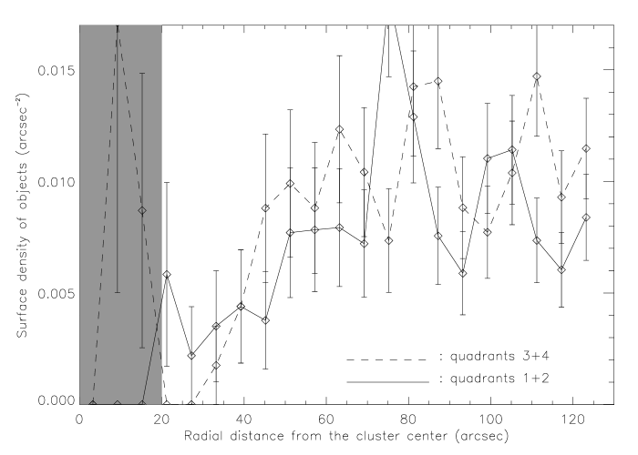
Figure 13: Depletion curves obtained in the I band for $\theta=0^{\circ}$ (top), $\theta=-10^{\circ}$ (middle) and $\theta=-20^{\circ}$ (bottom). The radial step has been reduced to 6″ only for a more accurate localisation of the minima

We have also used the depletion effect to determine the orientation of the main axis and the ellipticity of MS1008–1224. For this purpose, we divided the area of the FORS field into four quadrants where quadrants 1 and 2 are in opposition, and we performed the counts for radial distances from the cluster center to 130″ (Fig. 9). The positions of the four quadrants are marked by $\theta$, the clockwise angle between the North-South axis and the median of quadrant 1. We then computed the depletion curves corresponding to the counts in quadrants 1+2 and 3+4. We varied $\theta$ and followed the shift of the minimum position of the depletion area of the two curves. We can measure the orientation of the two main axis when the shift between the two minima is maximum. For this value of $\theta$, the relative positions of the two minima give the main axis ratio and consequently the ellipticity. The results, obtained from I-band data only, are similar in the others bands. From the I-band data only, we found $\theta=-10^{\circ}\pm 3^{\circ}$ and an ellipticity of $\epsilon=0.18\pm 0.04$ (Fig. 13). These results agree well with the mass map orientation derived from weak lensing as well as the galaxy number density map Athreya et al. (2000). A small discrepancy arrises with the X-ray gas distribution which orientation is shifted a few 10 to 20 degrees West from our measure Lewis et al. (1999). But globally, all these results are consistent within each other.

6 Conclusions

The gravitational magnification by cluster lenses represents an effective tool to probe the distant universe and the mass distribution in the lenses. The first aim of this paper was to study the effects of lens mass profile model parameters on the typical features of depletion curves. We have also attempted to characterize some features associated with the background redshift distribution of the galaxies. Models were constructed in three bands covering a large spectral range and by using five different lens models.

Our simulations agree well with very deep and high quality images of the cluster MS1008–1224 obtained with the VLT and FORS. The depletion effect is clearly seen in this cluster, and we have fitted its radial variation with several sets of mass profiles. The results are quite satisfying as we are able to constrain the mass profile up to a reasonable distance from the center (about 200″, or equivalently 1.1 $h_{50}^{-1}$ Mpc). Our results marginally favor the NFW mass profile over the isothermal profile, and more significantly reject a power-law distribution, essentially because of the steep rise of the depletion curve just after its minimum. Note that this region corresponds to the “intermediate” lensing regime, where shear measurements are more difficult to relate to the mass distribution. We have also studied the shape of the depletion area, which is easy to relate to the ellipticity of the mass distribution. We were then able to constrain the ellipticity and orientation of the potential of MS1008–1224 with a good accuracy.

This preliminary study highlights the need for additional exploration of several issues not fully explored in the present paper. For example, the question of clustering of the background sources still remains, although in the case of MS1008–1224, we have shown how it can be partly eliminated. Schneider et al. (2000) also mention this problem and insist on the fact that, at deep magnitudes, the two point correlation function of the sources is still quite uncertain, but a positive signal does not seem to extend much above $\sim$ 1 ″. More quantitatively, we can use the most recent measures of the two point correlation function from the HDF-South Fynbo et al. (2000). At the magnitude limits used in our paper, this correlation function does not exceed a few percent for an angular separation of 10″, typical of our bin size. Previous measurements were less optimistic in the sense that their values attained 8 to 10 % at 10″, even at very faint magnitudes. But although there is still only poor knowledge of the amplitude of the correlation function at the faintest levels, we can hope that the effect will not be dramatic in our studies of the magnification bias, provided we retain a reasonable bin size at several arcseconds, to wash out most of the inhomogeneities.

Following preliminary approaches from the observational point of view Taylor et al. (1998); Athreya et al. (2000) or a more theoretical one Schneider et al. (2000), one now clearly needs to extensively and quantitatively compare the weak lensing approach with the magnification bias. In particular, with the new facilities of deep wide-field imaging presently available, most of the difficulties related to a small field-of-view can be overcome: for weak lensing measurement, a complete mass reconstruction requires shear measurements up to the “no-shear” region in the outer parts of the cluster to integrate the mass inwards. The absolute normalization of the field number counts for the magnification bias can also be estimated outside the cluster, in exactly the same observing conditions (filter, magnitude limit, seeing, …), giving an absolute calibration of the depletion effect.

Moreover, the full 2D mass reconstruction of the cluster from the depletion signal alone should be tested. As the signal is directly related to the magnification $\mu(\@vec{r})$, and then to $\kappa(\@vec{r})$ and $\gamma(\@vec{r})$, it should be in principle feasible to invert the depletion map to produce a non-parametric mass map. In practice, the reconstruction is simpler as soon as the shear $\gamma$ becomes small, because in that case $\mu$ and $\kappa$ are simply linearly related. In any case, we have shown in this paper that it is rather easy to reach the outer parts of the cluster up to Mpc scales. This is quite similar to what can be done with deep X-ray maps for intermediate redshift clusters Soucail et al. (2000). We want to insist on the fact that the magnification bias effect is easy to detect from the observational point of view because it is less sensitive to seeing conditions or to geometrical distortions of the instruments than are shear measurements Broadhurst et al. (1995); Fort et al. (1997). It only requires deeper observations, not necessarily in photometric conditions, provided one is able to reach the outer parts of the cluster to normalise the number counts. In order to improve the mass reconstruction, one may progress with the help of photometric redshifts, quite useful for faint objects, to constrain the redshift distribution of the sources Pelló et al. (1999); Bolzonella et al. (2000). This approach might also be useful in order to limit the influence of large scale over-density fluctuations when evaluating the magnification and the asymptotic limit of the depletion curves. This of course requires deep multi-color photometry, such as the one obtained on MS1008–1224. Extending this study up to large-scale structures (LSS) would probably be more difficult to implement as compared to the search for cosmic shear Van Waerbeke et al. (2000), and the depletion effect should be restricted to cluster scales, at least with the simple method used in this paper.

Finally, one of our initial prospects was to try to constrain the background redshift distribution with multi-wavelength observations of the depletion effect. We have shown that this is quite a difficult task as the wavelength dependence of the depletion curves is a kind of second order effect. Nevertheless, this may be an interesting point to explore at other wavelengths, where the background redshift distribution is quite different than in the optical. For example, deep ISO observations in the mid-IR of a few cluster lenses Altieri et al. (1999) may represent an extension of our analysis, as well as submm observations with SCUBA, provided enough sources are detected behind the lenses for a statistical analysis. Another possibility would be to address the question of the nature of the X-ray background sources and their redshift distribution through deep and high resolution observations of clusters with the new X-ray satellites Chandra and XMM Refregier and Loeb (1997).