A Numerical Simulation of the Reconnection Layer in 2D Resistive MHD

Abstract

In this paper we present a two-dimensional, time dependent, numerical simulation of a reconnection current layer in incompressible resistive magnetohydrodynamics with uniform resistivity in the limit of very large Lundquist numbers. We use realistic boundary conditions derived consistently from the outside magnetic field, and we also take into account the effect of the back pressure from flow into the the separatrix region. We find that within a few Alfvén times the system evolves from an arbitrary initial state to a steady state consistent with the Sweet–Parker model, even if the initial state is Petschek-like.

PACS Numbers: 52.30.Jb, 96.60.Rd, 47.15.Cb.

1 Introduction

Magnetic reconnection is of great interest in many space and laboratory plasmas [1, 2], and has been studied extensively for more than four decades. The most important question is that of the reconnection rate. The process of magnetic reconnection, is so complex, however, that this question is still not completely resolved, even within the simplest possible canonical model: two-dimensional (2D) incompressible resistive magnetohydrodynamics (MHD) with uniform resistivity $\eta$ in the limit of $S\rightarrow\infty$ (where $S=V_{A}L/\eta$ is the global Lundquist number, $L$ being the half-length of the reconnection layer). Historically, there were two drastically different estimates for the reconnection rate: the Sweet–Parker model [3, 4] gave a rather slow reconnection rate ($E_{\rm SP}\sim S^{-1/2}$), while the Petschek [5] model gave any reconnection rate in the range from $E_{\rm SP}$ up to the fast maximum Petschek rate $E_{\rm Petschek}\sim 1/\log S$. Up until the present it was still unclear whether Petschek-like reconnection faster than Sweet–Parker reconnection is possible. Biskamp’s simulations [6] are very persuasive that, in resistive MHD, the rate is generally that of Sweet–Parker. Still, his simulations are for $S$ in the range of a few thousand, and his boundary conditions are somewhat tailored to the reconnection rate he desires, the strength of the field and the length of layer adjusting to yield the Sweet–Parker rate. Thus, a more systematic boundary layer analysis is desirable to really settle the question. In particular, one needs an elaborate and detailed picture of the reconnection current layer — namely, a picture that features a realistic model for the variation of the outside magnetic field along the layer, and realistic 2D profiles of the plasma parameters inside the layer.

The development of such a framework is the main goal of the present paper. We believe that the methods developed in this paper are rather universal and can be applied to a very broad class of reconnecting systems that include more realistic physics. However, for definiteness and clarity we keep in mind a particular global geometry, that presented in Fig. 1 (although we do not use it explicitly in our present analysis). This Figure shows the situation somewhere in the middle of the process of merging of two plasma cylinders. Regions I and II are ideal MHD regions: regions I represent unreconnected flux, and region II represents reconnected flux. The two regions I are separated by the very narrow reconnection current layer. Plasma from regions I enters the reconnection layer and gets accelerated along the layer, finally entering the separatrix region, also between regions I and II. In general, both the reconnection layer and the separatrix region require resistive treatment.

The plasma entering the separatrix from the reconnection layer is traveling at nearly the Alfvén speed. It crashes into the plasma at rest on the separatrix lines, that has not passed through the reconnection layer, but which got there by direct ${\bf E\times B}$ motion across the lines as the position of the separatrix changed by reconnection. This crash generates considerable heat, and hence back pressure on the reconnection layer. However, the separatrix region is continually in transition since different plasma occupies it as the reconnection proceeds so that the heated plasma is moved into the reconnected region. Thus, the plasma encountered by the outflowing reconnected plasma is continually refreshed and can always be taken initially at rest. Therefore, there is a time delay before the back reaction sets in. In our paper, we attempt to model this dynamical behavior of the separatrix plasma as accurately as possible.

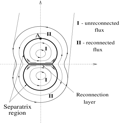
Figure 1: The global geometry.

In the limit $S\rightarrow\infty$ the reconnection rate is slow compared with the Alfvén time $\tau_{A}=L/V_{A}$, which allows one to break the whole problem into the global problem and the local problem. In a previous paper Ref. [7], we argued that on the global scale (i.e., on the scale of order the half-length of the layer $L$) the time evolution of the reconnecting system can be described as a sequence of magnetostatic equilibria. In paper [8] we explained that the role of the global solution is to give the general geometry of the reconnecting system, the position and the length of the reconnection layer and of the separatrix, and the boundary conditions for the local problem (which, in turn, determines the reconnection rate). These boundary conditions are expressed in terms of the outside magnetic field $B_{y,0}(y)$, where $y$ is the direction along the layer. In particular, $B_{y,0}(y)$ provides the characteristic global scales: the half-length of the layer $L$, defined as the point where $B_{y,0}(y)$ has minimum, and the global Alfvén speed, defined as $V_{A}=B_{y,0}(0)/\sqrt{4\pi\rho}$. It is important to understand that the global solution is essentially independent of the local reconnection physics.

In this paper we study the local problem concerning the reconnection layer itself. Our main goal here is to determine the internal structure of a steady state reconnection current layer (i.e., to find the 2D profiles of plasma velocity and magnetic field), and the reconnection rate represented by the (uniform) electric field $E$. Our most important result is that, in the case of uniform resistivity, there is a unique stable steady-state solution, and this is essentially the Sweet–Parker solution. We show that Petschek’s solution (which is not unique and supposedly encompasses a variety of reconnection solutions from that of Sweet and Parker to a solution reconnecting at almost the Alfvén speed) actually relaxes to the single Sweet-Parker solution.

First, in Section 2 we discuss the assumptions of our physical model of the layer in some detail. Then, in Section 3 we introduce the rescaled equations representing the mathematical model of our problem. In Section 4 we present our numerical simulations. And, finally, in Section 5 we give our conclusions.

2 Physical Model

By the local problem we mean the analysis of the internal structure of the reconnection layer and the separatrix layer, which is necessary for the determination of the reconnection rate. Since in ideal MHD these layers are current sheets of zero thickness, resolving their inner structure cannot be done in this ideal framework and requires the addition of some new nonideal physics.

Historically, most important, and conceptually most interesting for the purpose of resolving the current layer, is the inclusion of small resistivity. The model in which the only nonideal effect is that of the resistivity appears to be the simplest model with the minimal required complexity needed to resolve the current density singularity of an ideal MHD solution.

Thus, in this analysis we assume that the only new nonideal physical process is small constant and uniform resistivity $\eta$ (and perhaps viscosity $\nu$; see discussion below).

The inclusion of the small resistivity means the introduction of a new dimensionless small parameter associated with it, namely the inverse Lundquist number $S^{-1}=\eta/LV_{A}\ll 1$, which is considered the primary small parameter of the problem. This means that we are interested in studying the case of $S\rightarrow\infty$, and we want to determine how the parameters of the layer, such as its thickness and the reconnection rate, scale with $S$ in the leading order. As we shall see in the next section, making use of this small parameter helps to simplify the problem significantly while keeping all essential features, such as the two-dimensional nature of the problem, intact.

The next assumption we make concerns a steady state. The steady-state condition means that parameters of the current layer as well as the boundary conditions change very slowly compared with the global Alfvén time, which is the characteristic time spent by a fluid element inside the reconnection layer. A very important consequence of the steady-state condition in 2D geometry is that, due to the Maxwell equation $\nabla\times{\bf E}=-(1/c)\ \partial{\bf B}/\partial t$, the $z$ component of the electric field is uniform: $E_{z}(x,y)=E={\rm const}$.

As for the plasma viscosity, it does not seem to be necessary to include it, because viscosity, unlike resistivity, does not play any role in the actual breaking the lines of force. However, we always include a small constant and uniform viscosity $\nu$ for two reasons. First, in our numerical simulations we include it for numerical stability. The second and more important reason is that the consideration of very small (even compared with the resistivity) viscosity is useful to correctly understand some important features of the magnetic field configuration at the very center of the current layer (see Ref. [9]).

Next, most of the classical models of reconnection, including both Sweet–Parker and Petschek, assume that the outside merging magnetic field is uniform. But this assumption actually prohibits one from formulating the problem in a mathematically complete and consistent manner, because the downstream boundary conditions for the flow cannot be correctly specified. In this quasi-one-dimensional framework, there is no natural end of the layer; in particular, there is no way to define the global scale $L$. This, in turn, makes all attempts to get some scalings for the reconnection rate with the Lundquist number essentially meaningless, since the definition of the Lundquist number involves $L$.

Now, in our paper a generic and more or less representative variation of the outside magnetic field $B_{y,0}(y)$ along the layer and along the separatrix [where it is called $B_{s,1}(l)$] is included as an integral part of the problem. In particular, the global scale (the half-width $L$ of the layer) is defined naturally as the distance along the midplane from the center of the current layer to one of the two endpoints — i.e., the points where the outside magnetic field goes through a minimum and where the separatrices branch off the midplane $x=0$. In fact, this global scale is the characteristic scale for the function $B_{y,0}(y)$. Since this function is determined by the global ideal MHD solution (see Ref. [8]), the scale $L$ is, by definition, independent of the physics of the resistive layer.

Thus, the nonuniformity of the outside magnetic field along the layer makes the problem essentially two-dimensional (rather than one-dimensional). One practically important consequence of this fact is that the problem becomes much more complicated mathematically, so that one has to abandon any hope for a nice analytical solution and to resort to numerical simulation instead.

Thus, the physical model of the reconnection layer that we are going to use in this paper for treating the local problem, can be summarized as

two-dimensional, steady-state, incompressible, resistive MHD with constant and uniform resistivity (and perhaps viscosity) in the limit of very large Lundquist number.

Perfect mirror symmetry is assumed with respect to both the $x$ axis and the $y$ axis.

We call this model the canonical reconnection layer model.

When considering the local problem in this model, we use the global scale in the $y$ direction (along the layer), and the local scale in the $x$ direction (across the layer). The outside magnetic field $B_{y,0}(y)$ determined by the global solution here plays the role of a boundary condition at $x\rightarrow\infty$.

Finally, although in this section we talked only about the reconnection layer itself, the same physical model applies also to the separatrix layer.

3 System of Rescaled Equations

In accordance with our physical mode, we can now write down the set of two-dimensional steady-state fluid equations for our system. These equations are:

(i) The incompressibility condition:

$$\nabla\cdot{\bf v}={{\partial v_{x}}\over{\partial x}}+{{\partial v_{y}}\over{\partial y}}=0.$$

(ii) The $z$ component of Ohm’s law:

$$\eta j_{z}=E+v_{x}B_{y}-v_{y}B_{x},$$

where $E\equiv E_{z}={\rm const}$.

(iii) The equation of motion (with the viscosity):

$${\bf v}\cdot\nabla{\bf v}=-\nabla p+[{\bf j_{z}}\times{\bf B}]+\nu\nabla^{2}{\bf v},$$

where the density is set to one.

Now we take the crucial step in our analysis. We note that the reconnection problem is fundamentally a boundary layer problem, with $S^{-1}$ being the small parameter. This allows us to simplify our MHD equations by performing a rescaling procedure[10] inside the reconnection layer, to make rescaled resistivity equal to unity. This can be done in a natural way if one rescales the distances and the fields in the $y$ direction to the corresponding global values (i.e., the length of the layer $L$, the outside magnetic field just above the center of the layer $B_{y,0}(0)$, and the corresponding Alfvén speed $V_{A}$), while rescaling the distances in the $x$ direction and the $x$ components of the velocity and magnetic field to the corresponding local values:

$${y\over L}\rightarrow y,\qquad\qquad{x\over{\delta_{0}}}\rightarrow x,$$

$${v_{y}\over V_{A}}\rightarrow v_{y},\qquad\qquad{v_{x}\over{V_{A}\delta_{0}/L}}\rightarrow v_{x},$$

$${B_{y}\over{B_{y,0}(0)}}\rightarrow B_{y},\qquad\qquad{B_{x}\over{B_{y,0}(0)\delta_{0}/L}}\rightarrow B_{x},$$

$${p\over{B_{y,0}^{2}(0)/4\pi}}\rightarrow p,\qquad\qquad{E\over{B_{y,0}(0)V_{A}\delta_{0}/L}}\rightarrow E,$$

where $\delta_{0}\equiv LS^{-1/2}$ is the Sweet–Parker thickness of the current layer. Thus, one can see that the small scale $\delta_{0}$ emerges naturally as the thickness of the resistive boundary layer.

The viscosity $\nu$ is now rescaled as $\nu/\eta\rightarrow\nu$. We assume that it is at least as small as the resistivity [which means $\nu=O(\eta)$ or less], and most of the time (see Ref. [9]) we will be interested in the case of vanishing viscosity $\nu\rightarrow 0$ (which means $\nu\ll\eta$).

Now, all of the rescaled dimensionless quantities ($v_{x}$, $v_{y}$, $B_{x}$, $B_{y}$) are generally of order 1. Using the small parameter $\delta_{0}/L=S^{-1/2}\ll 1$, one can simplify the equations by writing them down in the leading nontrivial order in $\delta_{0}/L$. This way one neglects all unimportant corrections, keeping only the essential terms.

First, the incompressibility condition is written in rescaled quantities in exactly the same way as in the unrescaled quantities:

$${{\partial v_{x}}\over{\partial x}}+{{\partial v_{y}}\over{\partial y}}=0.$$

The $z$ component of the steady-state Ohm’s law can be written as

$$E={{\partial B_{y}}\over{\partial x}}-v_{x}B_{y}+v_{y}B_{x},$$

where the first term on the RHS is the resistive term.

Next, consider the equation of motion. Since all the velocities in the $x$ direction are small compared with the Alfvén speed, the inertial terms in the $x$ component of the equation of motion (3) are small, and this equation just gives one the pressure balance across the current sheet:

$${\partial\over{\partial x}}\left(p+{B_{y}^{2}\over 2}\right)=0,$$

which allows one to determine the pressure $p$ in terms of $B_{y}(x,y)$ once the pressure and the magnetic field $B_{y,0}(y)$ outside the reconnection layer are known. It is customary to set the pressure outside the layer to zero, so that

$$p(x,y)={{B_{y,0}^{2}(y)}\over 2}-{{B_{y}^{2}(x,y)}\over 2}.$$

(Of course, one can add a large constant to the pressure to enforce incompressibility. Since this constant cancels out of all our equations, we ignore it.)

Finally, one has the $y$ component of the equation of motion, with acceleration provided both by the pressure gradient force, and by magnetic forces, and with the viscous force:

$${\bf v}\cdot\nabla v_{y}=-{{\partial p}\over{\partial y}}+B_{x}{{\partial B_{y}}\over{\partial x}}+\nu{{\partial^{2}v_{y}}\over{\partial x^{2}}}.$$

It is interesting to note that almost everywhere in the layer the magnetic force $j_{z}B_{x}=B_{x}\partial_{x}B_{y}$ is actually just the $y$ component of the magnetic pressure gradient force $\nabla_{\perp}B^{2}/8\pi=\nabla B^{2}/8\pi-{\bf bb}\cdot\nabla B^{2}/8\pi$ where ${\bf b}$ is the unit vector along ${\bf B}$. The magnetic tension force $B^{2}{\bf b\cdot\nabla b}/4\pi$ is higher order everywhere except very close to the midplane (in a thin region where the unrescaled fields satisfy $B_{y}<B_{x}$).

We believe that this rescaling procedure captures all the important dynamical features of the reconnection process.

4 Numerical Simulations

In order to find the steady-state solution for the system, we designed a time dependent resistive MHD code for the main reconnection layer. This main code was supplemented by another code describing the separatrix, which is needed to provide the nearly correct downstream boundary conditions for the main code.

In Section 4.1 we describe the main code for the reconnection layer together with the boundary conditions. In Section 4.2 we discuss the different choices for the initial conditions used in the simulation. In Section 4.3 we present the model for the separatrix region that we have used in order to get the downstream boundary conditions for the main layer. In Section 4.4 we report the results of our numerical simulations. More details can be found in Ref. [10].

4.1 Numerical Scheme and Boundary Conditions

In order to approach the steady-state solution described by the system of rescaled equations (5), (6), (8), and (9), we followed the true time evolution of the system, starting with some initial conditions that will be described in Section 4.2.

The time evolution is described by the following two dynamic equations for the two dynamic variables $\Psi$ and $v_{y}$:

$${{\partial\Psi(x,y)}\over{\partial t}}=-\nabla\cdot({\bf v}\Psi)+{{\partial^{2}\Psi}\over{\partial x^{2}}}+\left(\eta_{y}{{\partial^{2}\Psi}\over{\partial y^{2}}}\right),$$

and

$${{\partial v_{y}}\over{\partial t}}=-\nabla\cdot({\bf v}v_{y})-{d\over{dy}}\left[{{B_{y,0}^{2}(y)}\over 2}\right]+\nabla\cdot({\bf B}B_{y})+\nu{{\partial^{2}v_{y}}\over{\partial x^{2}}}+\left(\nu_{y}{{\partial^{2}v_{y}}\over{\partial y^{2}}}\right).$$

These equations are written (using $\nabla\cdot{\bf v}=0$) in conservative form (i.e., in the form of conservation laws), which is preferable for numerical computations. Small artificial resistivity $\eta_{y}$ and viscosity $\nu_{y}$, acting in the $y$ direction, are added to provide numerical stability. Because they are small, these terms do not change the solution noticeably, as was verified in the runs. The natural unit of time in our simulations is the global Alfvén time $\tau_{A}=L/V_{A}$.

Once $v_{y}$ and $\Psi$ are known everywhere at a new time step, one can find all other variables. Namely, $B_{x}$ and $B_{y}$ are given by the derivatives of $\Psi$:

$$B_{x}=-{{\partial\Psi}\over{\partial y}},\qquad B_{y}={{\partial\Psi}\over{\partial x}},$$

and $v_{x}$ is obtained from the incompressibility condition by integrating $\partial v_{y}/\partial y$ in the $x$ direction starting from the midplane, where $v_{x}=0$ because of the symmetry:

$$v_{x}(x,y)=-\int_{0}^{x}{{\partial v_{y}}\over{\partial y}}dx.$$

We used the finite-difference method with centered derivatives (providing second order accuracy) in both the $x$ and the $y$ directions.

The time derivatives were one-sided. Our scheme was explicit in the $y$ direction, but in the $x$ direction the resistive term in Ohm’s law ($\partial^{2}\Psi/\partial x^{2}$) was treated implicitly, while all other terms were treated explicitly. This enabled us to speed up the computations.

We conducted the simulations on a rectangular grid ($i_{m}\times j_{m}$). Because of the symmetry, we considered only one quadrant (see Fig. 2).

Figure 2: Computational box used in the numerical simulation.

Now let us discuss the boundary conditions. There are four boundaries in the system: the upstream (or upper) boundary $x=x_{\rm lim}$, $0<y<y_{\rm lim}$, the downstream (or right) boundary $y=y_{\rm lim}$, $0<x<x_{\rm lim}$, and the two boundaries formed by the axes of symmetry: the lower boundary $x=0$, $0<y<y_{\rm lim}$, and the left boundary $y=0$, $0<x<x_{\rm lim}$. The flow enters through the upper boundary and leaves through the right boundary, so that there is no flow of plasma through the left and the lower boundaries. While the boundary conditions at the left and the lower boundaries come from simple symmetry conditions, the boundary conditions on the upper boundary and especially on the right boundary are more complicated, as we shall discuss below.

On the upper boundary, the boundary conditions come from matching with the ideal MHD solution in region I above the reconnection layer. In rescaled quantities, this matching should be done at $x\rightarrow\infty$. But since in a numerical simulation it is not possible to place a boundary of the computation box at infinity, we place it at some sufficiently large $x_{\rm lim}\gg 1$. The typical values of $x_{\rm lim}$ in our simulations were $x_{\rm lim}\simeq 4-8$.

From the ideal solution in region I we know that, as $x\rightarrow\infty$, $v_{y}\rightarrow 0$ (meaning $v_{y}\ll V_{A}$) and $B_{y}\rightarrow B_{y,0}(y)$, which is prescribed. It turns out that, since the upper boundary is placed not at infinity but at some finite (although large) $x_{\rm lim}$, it is better, for numerical reasons, to choose ${\partial v_{y}}/{\partial x}(x_{\rm lim})=0$ instead of $v_{y}(x_{\rm lim})=0$.

As for the magnetic field, we just set ${\partial\Psi}/{\partial x}(x_{\rm lim})=B_{y,0}(y)$. The function $B_{y,0}(y)$ depends on the external boundary and the thermodynamics of the global solution as well as the amount of reconnected flux. Rather than make use of a specific global solution we choose a generic one since the physics in the reconnection layer should be the same. However, near $y=L$ (the end of the reconnection layer which terminates in a cusp geometry we must employ the square-root behavior derived in Ref. [8], which any global solution must have. Thus, in our numerical simulations we typically took

$$B_{y,0}(y)=B_{0}+(1-B_{0})\sqrt{1-y^{2}},$$

consistent with the cusp solution (see Ref. [8]). The value $B_{0}$ of the outside magnetic field $B_{y,0}$ at the endpoint $y=1$ typically was taken to be $B_{0}=0.2$ or $B_{0}=0.3$ [the magnetic field is normalized so that $B_{y,0}(0)=1$].

This choice of boundary conditions worked well in our simulations. In particular, the behavior of the solution near the upper boundary was smooth, and the solution deep inside the reconnection layer did not depend on the exact position of the upper boundary.

At the lower boundary $x=0$, the boundary conditions come naturally from the requirement that both $v_{y}$ and $\Psi$ be symmetric with respect to the midplane. Thus,

$${{\partial v_{y}}\over{\partial x}}=0\qquad{\rm and}\qquad B_{y}={{\partial\Psi}\over{\partial x}}=0\qquad(x=0),$$

and also $v_{x}(0,y)=0$.

Here, however, we would like to make one remark. The boundary condition for ${\partial v_{y}/}{\partial x}$ at $x=0$ is needed only when one includes the viscous term $\nu\partial^{2}v_{y}/\partial x^{2}$ in the equation of motion. If one does not keep this term, then this equation contains only first derivatives of $v_{y}$ in the $x$ direction, so one needs only one condition, which can be set at the upper boundary. In our simulations, however, we always include viscosity (usually small, but not zero), both for numerical reasons and in order to resolve the behavior near the midplane (see Ref. [9]).

The boundary conditions at the left boundary are similar to those on the lower boundary. They follow from symmetry and are rather straightforward:

$$v_{y}(x,0)=0,\qquad{\rm and}\qquad B_{x}(x,0)=0.$$

Now consider the right (or downstream) boundary. We chose it at some point $y=y_{\rm lim}$ close to the endpoint (typically $y_{\rm lim}=0.9-1.0$). Then, one needs to specify the downstream boundary conditions on this boundary. This boundary is, in fact, the interface between the main layer and the endpoint region and the separatrix. The boundary conditions should describe the effect of the separatrix reacting back on the main layer, in particular the back pressure. We are not aware of any previous numerical or theoretical studies in which the role of the back pressure has been adequately investigated. The problem of how to set the boundary conditions on this boundary is rather nontrivial and its discussion is postponed until Section 4.3.

To summarize, the advantages of our approach to numerical simulation of the reconnection layer are the following:

1) First, the use of rescaled equations takes us directly into the realm of $S\rightarrow\infty$.

2) Second, this is an essentially 2D (rather than 1D) code that uses a realistic variation of the outside magnetic field along the layer. The position of the endpoint is clearly defined in terms of the function $B_{y,0}(y)$. We do not assume $B_{y,0}(y)={\rm const}$ as many people do.

3) We obtain the steady-state solution by following the true time evolution, and the rescaled equations are such that we do not give the boundary conditions for the incoming flow velocity at the upstream boundary. This is because the physical $v_{x}$ is small and its evolution is not determined from a dynamic equation of motion. Instead, the equation of motion in the $x$ direction simply degenerates into the vertical pressure balance, and $v_{x}$ is determined from the incompressibility condition. Thus, we do not specify $v_{x}(x_{\rm lim},y)$ as a boundary condition, which means that we do not prescribe the reconnection rate! The system itself determines what the reconnection rate should be! This is really a very important point.

The fact that we rescaled the $x$ coordinate using the Sweet–Parker scaling does not actually mean that we prescribe the Sweet–Parker reconnection rate. If the system wants to go at a faster rate, then it would try to develop some new characteristic structures, extending beyond $x_{\rm lim}$, and we should be able to see it.

4.2 Initial Conditions

We have performed several runs with different initial conditions consistent with our boundary conditions.

In some cases we started with a configuration qualitatively resembling the Sweet–Parker reconnection layer (see Figs. 3 and 4). These initial conditions can be written in the following analytical form:

$$B_{y}(x,y)=B_{y,0}(y)\tanh(x),$$

$$\Psi(x,y)=\Psi(0,y)+B_{y,0}(y)\log{\cosh{x}},$$

$$B_{x}(x,y)=-{{\partial\Psi}\over{\partial y}},$$

where we took the outside magnetic field $B_{y,0}(y)$ in the form (14), and the variation of the magnetic flux on the midplane as

$$\Psi(0,y)=-{\pi\over 4}y^{2}.$$

The initial velocity was taken in the form

$$v_{x}(x,y)=-{E_{0}\over{B_{y,0}(y)}}\tanh(x),$$

and

$$v_{y}(x,y)=-\int_{0}^{y}{{\partial v_{x}}\over{\partial x}}dy,$$

where the initial outside electric field $E_{0}$ varied but typically was of order one. We call the initial conditions described by the set of Eqs. (4.17)–(4.22) the Sweet–Parker-like initial conditions.

Figure 3: Contour plot of the magnetic field for Sweet–Parker-like initial conditions.

Figure 4: Plots of $j(x)$ for different values of $y$ at $t=0$ for Sweet–Parker-like initial conditions.

In other runs we wanted to see whether the system would want to go with the faster reconnection rate and whether it would develop the Petschek-like structures.

(It should be observed that Petschek, in his original paper, did not specify a unique reconnection rate. Instead his reconnection rate depended on the length of the dissipation region $y_{*}$, and his reconnection velocity was $v_{\rm rec}=(\sqrt{L/y_{*}})V_{A}/\sqrt{S}$. For example, the choice $y_{*}=L$ gives the Sweet-Parker rate. The usually quoted Petschek reconnection velocity, $v_{\rm Petschek}\sim V_{A}/\log{S}$, was obtained by him when he took the minimum possible value for $y_{*}$ that would not seriously perturb the global solution. Furthermore, it is possible to include Petschek’s shocks inside the boundary layer as indeed he did.)

We conjectured that if the system wants to go at a faster reconnection rate than that of Sweet–Parker, then it would at least be able to go at a rate twice as fast(i.e., $y_{*}=L/4$). Therefore, we carried out several runs where at $t=0$ we set up a Petschek-like structure (see Figs. 5, 6, and 7) described by the following expressions:

$$\Psi(0,y)=-{1\over M}\log{\cosh(z_{0})},$$

$$B_{y}(x,y)=B_{y,0}(y)\left[{{\tanh(z_{1})+\tanh(z_{2})}\over 2}\right],$$

$$\Psi(x,y)=\Psi(0,y)+{{B_{y,0}(y)}\over{2M}}\ [\log{\cosh(z_{1})}+\log{\cosh(z_{2})}-2\log{\cosh(z_{0})}],$$

$$B_{x}(x,y)=-{{\partial\Psi}\over{\partial y}},$$

$$v_{y}(x,y)={{\tanh(z_{1})-\tanh(z_{2})}\over 2},$$

$$v_{x}(x,y)=-M\left[{{\tanh(z_{1})+\tanh(z_{2})}\over 2}\right],$$

where $z_{0}=M^{2}y$, $z_{1}=Mx+M^{2}y$, and $z_{2}=Mx-M^{2}y$, and where the parameter $M$ corresponds to the initial reconnection rate in terms of the Sweet–Parker reconnection rate. It describes how well pronounced the Petschek-like structure is ($M$ would correspond to $\sqrt{L/y_{*}}$ in Petschek’s notation). Typically $M$ was chosen to be 2 or 3. We call the initial conditions described by the set of Eqs. (23)–(28) the Petschek-like initial conditions.

Figure 5: Contour plot of magnetic field at $t=0$ for the Petschek-like initial conditions.

Figure 6: The current density $j(x,y)$ at $t=0$ for Petschek-like initial conditions (all four quadrants are shown for clarity).

Figure 7: Plots of $j(x)$ for different values of $y$ at $t=0$ for the Petschek-like initial conditions.

4.3 The Downstream Boundary Conditions and the Model for the Separatrix Region

The downstream boundary $y=y_{\rm lim}$ is the interface between the main layer and the separatrix region. The boundary conditions at this boundary cannot be given in a simple closed form. Instead, they require matching with the solution in the separatrix region, which itself is just as complicated as the main layer. Therefore, we have developed a supplemental numerical procedure for the separatrix region.

To make the situation more tractable, we have adopted simplified physical model for the separatrix — namely, a model in which the resistive and the viscous terms are omitted, and hence the magnetic field is frozen into the plasma. Even though this model does not describe the separatrix completely accurately, it should give one a qualitatively correct picture of the influence of the separatrix region back on the main layer, and thus sufficiently reasonable downstream boundary conditions for the main layer. In particular, our model includes the effects of the back pressure that the separatrix exerts on the main layer.

We follow one given field line as it moves across the separatrix of length $L_{s}$ as described in the introduction. This field line is described in terms of two functions: the magnetic field $B(l,t)$, and the parallel velocity $v(l,t)\equiv v_{\parallel}(l,t)$. Here $l$ is the length measured along the field line, starting from the boundary between the separatrix and the main layer ($l=0$ or $y=y_{\rm lim}$), and ending at the reflection point A at the top of Fig. 1 ($l=L_{s}$).

Now, the time evolution in this one-dimensional problem corresponds to the perpendicular motion of the field line through the separatrix region. The new time variable $t$ represents the relative position of the field line in real 2D space with respect to other field lines, and there is a one-to-one correspondence between the time $t$ and the $x$ position of the footpoint (the point where the field line intersects the boundary $y=y_{\rm lim}$) of this field line. This correspondence between $t$ and $x$ is given by the $x$ component of the velocity of the field line, $v_{xs}\equiv-E/B_{y}(x,y_{\rm lim})<0$ ($x$ decreases as $t$ increases), and by the initial condition that $x=x_{\rm lim}$ at $t=0$. We stop the simulation of the separatrix at the moment $t$ when $x(t)$ becomes zero — i.e., when the midplane is reached. A substantial advantage of this model is that one actually does not need to know where the field line is in real 2D space! The only thing one does need to know about the position of the field line in order to set up the downstream boundary conditions for the main layer is where it connects to the main layer — i.e., what is the value of the coordinate $x$ at the point where the field line intersects the downstream boundary $y=y_{\rm lim}$ (i.e., the footpoint).

The boundary conditions on the upper boundary of the separatrix are $v(l)=0$ and $B(l)=B_{s1}(l)$, where $B_{s1}(l)$ is the field outside the separatrix in the upstream region given by the global ideal MHD solution, as explained in Ref. [8]. In our simulation we took this outside field in the form

$$B_{s,I}(l)=\sqrt{B_{0}^{2}+{{C^{2}l}\over L_{s}}\left(1-{l\over{2L_{s}}}\right)}.$$

Now these conditions become the initial conditions at $t=0$ for our 1D (plus time) problem concerning this one field line.

As in the main layer, we use here an explicit (in $l$) code with centered differences for convective derivatives in the $l$ direction. The boundary conditions at the right boundary $l=L_{s}$ (the reflection point A on Fig. 1) come from the condition of symmetry with respect to this point ($l=L_{s}$):

$$v(L_{s},t)=0,\qquad{{\partial B}\over{\partial l}}(L_{s},t)=0.$$

The other pair of boundary conditions is given at the left (incoming) boundary $l=0$ and is provided by the main layer in terms of the values of $v_{y}(x,y_{\rm lim})$ and $B_{y}(x,y_{lim})$. Assuming that the steady state in the main layer has already been achieved, these boundary conditions are constant in time in the laboratory frame, but in the frame moving along together with the field line, they are now time-dependent.

Since at the boundary $y=y_{\rm lim}$ the layer is still essentially straight, and the field lines (except those few very close to the midplane, which are ignored) are also almost straight, then the absolute value of the magnetic field $B$ is almost exactly equal to $B_{y}$ and the parallel velocity $v$ is almost exactly equal to $v_{y}$. Therefore, the matching conditions at this boundary are $B_{y}=B$, $v_{y}=v$.

As for the downstream (or lower) boundary, one really does not need to set any conditions there because the $x$ coordinate in our model corresponds to time and the new equations have only first-order time derivatives.

Now let us derive the differential equations for this model of the separatrix. The main idea in this derivation is that the convective term ${\bf v}_{\perp}\cdot\nabla_{\perp}$ is replaced by the time derivative $\partial/\partial t$. The natural unit of time in this model is the Alfvén time, the natural unit of distance in the $l$ direction is the global scale $L$, and that of the parallel velocity is the Alfvén velocity $V_{A}$.

First of all, one can apply this model only to the part of the separatrix where the field lines are not very strongly curved (i.e., where the radius of curvature of the field lines is of order $L$), the magnetic field itself is sufficiently strong (of order $B_{0}$ or at least $B\gg B_{1}=E/V_{A}$), and the perpendicular velocity $v_{\perp}$ (which in ideal MHD is equal to $E/B$) is small compared with the parallel velocity $v_{\parallel}=O(V_{A})$. Thus, the model is bound to fail in the very small region near the midplane where the real physical $B_{y}$ becomes comparable with $B_{x}$.

In the system of reference moving together with the field line in the direction perpendicular to ${\bf B}$, the (parallel component of) the magnetic induction equation becomes

$$\dot{B}={{\partial B}\over{\partial t}}=B{\partial\over{\partial l}}v-v{\partial\over{\partial l}}B,$$

and the parallel equation of motion becomes

$${{\partial v}\over{\partial t}}=-v{{\partial v}\over{\partial l}}-{\partial\over{\partial l}}\left[{B_{s1}^{2}(l)\over 2}-{B^{2}(l,t)\over 2}\right].$$

Eq. (32) is equivalent to Eqs. (7) and (11). Physically, the force parallel to ${\bf B}$ is the pressure gradient force which can be expressed in terms of $B$ by Eq. (7). It is interesting to note that, while the fluid in the initial problem was incompressible, in this 1D problem the motion is effectively not incompressible (${\partial v/\partial l}\neq 0$), and the thickness of the flux tube ($\sim 1/B$) plays the role of density.

Now let us see how the back pressure from the separatrix acts on the main layer.

As the field line moves, the incoming velocity $v(l=0,t)$ increases from almost zero at $t=0$ to about the Alfvén velocity, and the incoming magnetic field $B(l=0,t)$ drops from $B_{0}$ to zero at the midplane. Therefore, there is a point $x=x_{c}$ somewhere in the middle of the left boundary of the separatrix where the incoming flow becomes locally super-Alfvénic ($v>B$). The propagation of information with respect to the fluid in our model occurs at the local Alfvén speed by the means of two characteristics $dl/dt=v\pm B$. For $x>x_{c}$ ($v<B$), one characteristic goes from the left boundary $l=0$ ($y=y_{\rm lim}$) towards the right boundary, while the other characteristic goes from the upper boundary $x=x_{\rm lim}$ towards the left boundary, carrying information about the pressure and the flow in the separatrix to the main layer. This means that, for $x>x_{c}$, the layer “feels” the effect of the separatrix in the form of the back pressure coming from the previously undisturbed fluid in the separatrix region. This back pressure is found to have some stabilizing effect, making the solution deep inside the main layer independent of $x_{\rm lim}$ and almost independent of the position $y_{\rm lim}$ of the downstream boundary (where the separatrix and the main layer solutions are matched).

After the field line crosses the point $x=x_{c}$, the flow becomes super-Alfvénic and the characteristic $dl/dt=v-B>0$ is deviated away from the left boundary back into the separatrix region. Now both characteristics come out of the left boundary and there is no propagation of information from the separatrix region into the main layer. This also means that when the field line reaches the vicinity of the midplane $x=0$ and the description of the separatrix region as a region of almost straight field lines fails, it does not matter much, because the flow at this point is very strongly super-Alfvénic and the main layer does not feel what happens downstream. We would like to remark that in our simulations we have not observed any shock formation in the separatrix.

Of course, this picture of the flow of information is valid only in this ideal MHD model. In the real situation with resistivity, there is always propagation of information upstream due to the resistive diffusion.

To summarize, the model of the separatrix region presented here has two main drawbacks. First, it describes an ideal MHD separatrix. Second, it assumes that the boundary conditions on the incoming boundary $l=0$ ($y=y_{\rm lim}$) are stationary (i.e., that the main layer has already reached the steady state). (This second objection can be removed if the main layer is evolved with right hand boundary conditions changing in step with the separatrix solution and vice versa, but this would involve a longer simulation.) In addition, the model is valid only when the field lines are essentially straight, as discussed above (the region where this assumption breaks down is discussed in Ref. [10]). Despite all that, however, we feel that this model provides a qualitatively correct picture of the dynamics in the separatrix region in the steady state, and thus gives us sufficiently reasonable downstream boundary conditions for the main layer.

4.4 Results of the Simulations

Now let us present and discuss the results of our numerical simulations.

We found that, after a transient period of a few Alfvén times, the system reaches a steady state that is independent of the initial configuration.

In particular, when we start with a Petschek-like initial configuration (described in Section 4.2), the high velocity flow rapidly sweeps away the transverse magnetic field $B_{x}$ (see Fig. 8). This is important, because, for a Petschek-like configuration to exist, the transverse component of the magnetic field on the midplane, $B_{x}(0,y)$, must be large enough to be able to sustain the Petschek shocks in the field reversal region. For this to happen, has to rise rapidly with $y$ inside a very short diffusion region, $B_{x}(0,y)$ $y<y_{*}\ll L$ (in the case $M=2$, presented in Fig. 8, $y_{*}=L/4$), to reach a certain large value ($B_{x}=2$ for $M=2$) for $y_{*}\ll y<L$. While the transverse magnetic flux is being swept away by the plasma flow, it is being regenerated by the merging of the $B_{y}$ field, but only at a certain rate and only on a global scale in the $y$-direction, related to the nonuniformity of the outside magnetic field $B_{y,0}(y)$, as discussed in Refs. [1] and [10]. As a result, the initial Petschek-like structure is destroyed, and the inflow of the magnetic flux through the upper boundary drops in a fraction of one Alfvén time. Then, after a transient period, the system reaches a steady state consistent with the Sweet–Parker model.

Figure 8: The time evolution of the variation of the transverse magnetic field $B_{x}(0,y)$ along the midplane $x=0$ for the Petschek-like initial conditions.

In general, the transient period typically lasts a few Alfvén times, during which the incoming electric field can oscillate around its final steady-state value. These oscillations have a period of order $\tau_{A}$, and a decay time also of the same order. After several $\tau_{A}$, the electric field becomes constant and uniform throughout the computational domain and the system approaches steady state. We terminate our simulations typically after 5 or 10 Alfvén times. The time evolution of the incoming electric field [i.e., $E(x=x_{\rm lim},0)(t)$] for different choices of the initial conditions is represented in Figs. 9 and 10.

Figure 9: The time evolution of the electric field $E$ at the point $x=x_{\rm lim}$, $y=y_{\rm lim}$ for the Sweet–Parker-like initial conditions with $E_{0}=1.0$.

Figure 10: The time evolution of the electric field $E$ at the point $x=x_{\rm lim}$, $y=y_{\rm lim}$ for the Petschek-like initial conditions with $M=2$ (corresponding to $E_{0}=2.0$).

We believe that the fact that we rescaled $x$ using the Sweet–Parker scaling does not mean that we prescribe the Sweet–Parker reconnection rate. Indeed, if the reconnecting system wanted to evolve towards Petschek’s fast reconnection, it would then try to develop some new characteristic structures, e.g., Petschek-like shocks, which we would be able to see. Note that, if Petschek is correct, then there should be a range of reconnection rates including those equal to any finite factor greater than one times the Sweet–Parker rate $E_{\rm SP}$. However, in our simulations we have demonstrated that there is only one stable solution and that it corresponds to $E=E_{\rm SP}$. In this sense we have demonstrated that Petschek must be wrong since reconnection can not even go a factor of two faster than Sweet–Parker, let alone almost the entire factor of $\sqrt{S}$. There seems no alternative to the conclusion that fast reconnection is impossible.

It is interesting that in Petschek’s original paper [5] the length of the central diffusion region $y_{*}$ is an undetermined parameter, and the reconnection velocity $v_{\rm rec}$ depends on this parameter as $V_{A}(L/y_{*})^{2}/\sqrt{S}$. If $y_{*}$ is taken as small as possible then Petschek finds that $v_{\rm rec}\sim V_{A}/\log(S)$. However, $y_{*}$ should be determined instead by balancing the generation of the transverse field $B_{x}$ against its loss by the Alfvénic flow (it should be remarked that Petschek did not discuss the origin of this transverse field in his paper). As we discussed above, this balance yields $y_{*}\approx L$, with the resulting unique rate equal to that of Sweet–Parker. This results are borne out by our time-dependent numerical simulations.

The final steady-state configuration represents the Sweet–Parker reconnection layer. This means that all the plasma parameters are of order one in the rescaled coordinates, and change on a scale of order $\delta_{0}$ in the $x$ direction and on a global scale $L$ in the $y$ direction. For our choice of boundary conditions [i.e., of the outside magnetic field $B_{y,0}(y)$], the reconnection rate in the steady state was $E=1.0\,E_{\rm SP}$, where $E_{\rm SP}\equiv\eta^{1/2}V_{A}B_{y,0}(0)$ is the typical Sweet–Parker reconnection rate.

The use of the time-dependent equations allows us not only to find the steady-state solution, but also to draw some conclusions about its stability. The Sweet–Parker solution was found to be stable and robust: it did not depend on the positions of the boundaries $x_{\rm lim}$, $y_{\rm lim}$ or on the small artificial resistivity and viscosity. Moreover, we found that it is fairly insensitive even with respect to the choice of the parameters describing the outside magnetic field, such as $B_{0}=B_{y,0}(1)$ (thus, $E$ varies by about 10% as $B_{0}$ changes from 0 to 0.3).

The steady-state Sweet–Parker solution is represented in Figs. 11, 12, 13, 14, and 15. This solution corresponds to the following set of the parameters describing the boundary conditions: $x_{\rm lim}=5.0$, $y_{\rm lim}=1.0$, $B_{0}=0.3$, $L_{s}=2.0$, $C=0.957$ [see Eqs. (14) and (29)]. In this particular run the values of the perpendicular viscosity $\nu$, and of the (artificial) resistivity and viscosity acting in the $y$ direction were $\nu=0.02$, $\eta_{y}=\nu_{y}=0.01$.

Figure 11: Contour plot of the steady-state magnetic field in the reconnection layer.

Figure 12: The current density $j(x,y)$ in the steady state (all four quadrants are shown for clarity).

Figure 13: Plots of $j$ as a function of $x$ for several different values of $y$ in the steady state.

Figure 14: Plots of $B_{y}$ as a function of $x$ for several different values of $y$ in the steady state.

Figure 15: Plots of $V_{y}$ as a function of $x$ for several different values of $y$ in the steady state.

There are several things that should be noted about this solution:

As can be seen from Fig. 13, the current density as a function of $x$ at any given value of $y$ peaks on the midplane $x=0$. This makes the solution qualitatively different from a Petschek-like configuration (see Fig. 7) in which the current density is concentrated in a shock-like structure off the midplane.

At any given $y$, the current density $j(x)$ rapidly goes to zero as $x\rightarrow\infty$, and $B_{y}(x,y)\rightarrow B_{y,0}(y)$ monotonically, which means that there is no flux pile up in front of the layer. The velocity $v_{y}$ does not quite go to zero at the upper boundary, but its value at $x=x_{\rm lim}$ is small and goes to zero as the artificial $\eta_{y},\nu_{y}\rightarrow 0$.

Next, the solution in the layer shows an essentially linear rise of $v_{y}$ and $B_{x}$ along the midplane $x=0$ (see Figs. 16 and 17). The linear behavior of $B_{x}(x=0,y)$ near $y=0$, contrary to the cubic behavior predicted by Priest and Cowley [11], was explained in Ref. [9] (together with the nonanalytic behavior of the solution near the midplane in the limit $\nu\rightarrow 0$).

Finally, $B_{x}$ exhibit a sharp change near the downstream boundary $y=y_{\rm lim}$, as can be seen in Figs. 17. This change is due to the fact that in the separatrix region we neglect the resistive term $\Psi_{xx}$, which is in fact finite. That is, the (perpendicular) resistivity effectively has a discontinuity across $y=y_{\rm lim}$: $\eta(y<y_{\rm lim})=1$ and $\eta(y>y_{\rm lim})=0$. This discontinuity in the equations also shows up in the solution, but it is smoothed out over some vicinity of $y_{\rm lim}$ by the artificial resistivity and viscosity in the $y$ direction. As these $\eta_{y}$, $\nu_{y}$ go to zero, the region of the rapid change near $y_{\rm lim}$ becomes smaller and smaller.

Figure 16: Plots of $v_{y}$ as a function of $y$ along the midplane $x=0$ in the steady state.

Figure 17: Plots of $B_{x}$ as a function of $y$ along the midplane $x=0$ in the steady state.

Let us add a few remarks about the role of the separatrix region in our simulations.

First, it appears that the destruction of the initially-set-up Petschek-like configuration and its conversion to the Sweet–Parker-like layer is so robust and happens so fast, that it is determined by the dynamics in the main layer and by its interaction with the upstream boundary conditions [i.e., with the scale of nonuniformity of the outside magnetic field $B_{y,0}(y)$]. As a consequence, it has nothing to do with the downstream boundary conditions (i.e., with the separatrix region). Therefore, the fact that our model of the separatrix does not describe the separatrix completely accurately seems to be unimportant, as far as the instability of the Petschek solution is concerned.

Thus, we believe that the separatrix region, while providing physically reasonable downstream boundary conditions for the main layer problem, does not really have a strong effect on the principal result that the stable steady-state solution is the Sweet–Parker layer with the Sweet–Parker reconnection rate. Still, we have to point out that for the solution of the problem to be really complete, one needs to build a better model of the separatrix region. Such a model would include real time dependence and resistivity, and also would treat the very near vicinity of the endpoint of the reconnection layer. A proper consideration of the endpoint region cannot be done in rescaled variables, and a further rescaling of variables and matching is needed.

5 Conclusions

To summarize, in this paper we present a definite systematic solution to a particular clear-cut, mathematically consistent problem concerning the internal structure of the reconnection layer within the canonical framework (incompressible 2D MHD with uniform resistivity) with the outside field $B_{y,0}(y)$ varying on the global scale along the layer. We have first derived a system of rescaled equations that should be valid in the limit $S\rightarrow\infty$. Then, we have developed a 2D resistive MHD code that followed the time evolution of the system in order to achieve the steady state.

We conclude that, under the assumptions of our model, the Petschek-like solutions are unstable and the system quickly evolves to the only stable steady-state solution corresponding to the Sweet–Parker reconnection layer. Thus, the Petschek mechanism for fast reconnection does not work in our model. The steady-state reconnection rate in our model problem is remarkably close to the Sweet–Parker value $E_{\rm SP}=B_{y,0}(0)V_{A}/\sqrt{S}$.

This main result is consistent with the results of simulations conducted by Biskamp[6] and also those by Ugai[12] and by Scholer[13]. It also agrees with the experimental results in the MRX experiment [14].

Finally, even though we draw our conclusions (about Petschek-like structures being unstable) only for this very specific model, this result is fundamentally important, because this model is the canonical framework typical of most models of magnetic reconnection, including both Sweet–Parker and Petschek. This framework is the simplest possible framework for a reconnection problem, and thus provides the necessary foundation on top of which one can add more complicated physical processes. Because the Sweet–Parker model with the classical (Spitzer) resistivity is known to be too slow to explain the very fast time scale for the energy release in solar flares, one has to look for physics beyond resistive MHD with the Spitzer resistivity. The inclusion of some new physical processes into the model (for example, locally enhanced anomalous resistivity is probably the most suitable candidate) would create a very different situation in which some Petschek-like structure with fast reconnection may be possible.

6 Acknowledgment

We are grateful to D. Biskamp, S. Cowley, T. Forbes, M. Meneguzzi, S. Jardin, M. Yamada, H. Ji, S. Boldyrev, and A. Schekochihin for several fruitful discussions. This work was supported by Charlotte Elizabeth Procter Fellowship, by the Department of Energy Contract No. DE-AC02-76-CHO-3073, and by NASA’s Astrophysical Program under Grant NAGW2419.

7 APPENDIX

We give a rough physical argument for why the length $L^{\prime}$ of the Petschek diffusion region must be of order the global length $L$, and correspondingly, why the Petschek reconnection rate must reduce to the Sweet–Parker rate.

The equation of motion for the $B_{x}$ field should have two terms: a loss term $-(v_{A}/L^{\prime})B_{x}$ , and a source term due to the nonuniform merging of the incoming $B_{y}$ field. An estimate for the size of this source term is as follows.

The boundary condition for the external field $B_{y}$ is determined globally by a field scaled to the global length $L$. For simplicity, we take this as

$$B_{y,\rm ext}=B_{0}(1-y^{2}/L^{2}),$$

and apply it over the length of the Petschek diffusion layer, $L^{\prime}\ll L$.

If the external field were entirely uniform, then the merging of the field in the diffusive region would be uniform and there would be no tendency to develop a $B_{x}$ field. If the boundary condition on $B_{y}$ is satisfied and $L^{\prime}\ll L$, the tendency to develop $B_{x}$ by nonuniform merging would be proportional to $L^{\prime 2}/L^{2}$, the nonuniformity of the external field. There are several terms leading to the generation of $B_{x}$, all of the same order of magnitude.

For example, consider the rate of generation of $B_{x}$ by the resistive diffusive velocity alone. Let the layer initially have only a $B_{y}$ field and be of uniform thickness $\delta$. Then $j\sim B_{y,\rm ext}/\delta$ is stronger at $y=0$ than at $y=L^{\prime}$ by the amount $B_{0}/\delta(L^{\prime 2}/L^{2})$, so the electric field $E=\eta j$ is correspondingly larger. Therefore, the rate at which lines enter at $y=0$ is larger by $\Delta\dot{\Psi}=(\eta/\delta)(L^{\prime 2}/L^{2})B_{0}$ than that at $y=L^{\prime}$.

These excess lines must turn from the $y$ direction to the $x$ direction and produce the $B_{x}$ field. Dividing this rate by $L^{\prime}$ we get the rate of generation of the $B_{x}$ field,

$$\dot{B}_{x}(generation)=(\eta/\delta_{0})(L^{\prime}/L^{2})B_{0}.$$

One can convince oneself that the other terms, that generate the $B_{x}$ field such as the variation in the layer thickness $\delta$, the variation in the $x$ velocity of the plasma, etc., are of the same order of magnitude. Thus, the above rate $(\eta/\delta)(L^{\prime 2}/L^{2})(B_{0}/L^{\prime})$ should give a rough positive upper bound to the regeneration rate of the $B_{x}$ field. Therefore, the $B_{x}$ field cannot be stronger than that given by the balance equation

$$\frac{dB_{x}}{dt}=-B_{x}\frac{V_{A}}{L^{\prime}}+\frac{\eta}{\delta}\frac{L^{\prime}}{L^{2}}B_{0}=0,$$

so $B_{x}=(\eta/\delta)(L^{\prime 2}/L^{2})B_{0}/V_{A}$. Now, according to Petschek, the emerging $B_{x}$ field drives the shocks at a speed $B_{x}/\sqrt{4\pi\rho}$ in the $x$ direction, which just balances the incoming plasma with velocity $v_{\rm rec}$.

Thus,

$$v_{\rm rec}=\frac{B_{x}}{\sqrt{4\pi\rho}}=\frac{\eta}{\delta}\frac{L^{\prime 2}}{L^{2}}$$

But we also have, from Petschek, $v_{\rm rec}=\eta/\delta_{0}$, so that

$$L^{\prime}=L,$$

and this reduces the Petschek reconnection rate

$$v_{\rm rec,Petschek}=\frac{V_{A}}{\sqrt{S}}\sqrt{\frac{L^{\prime}}{L}},$$

to the Sweet–Parker rate.

References

- [1] R. M. Kulsrud, Phys. Plasmas, 5, 1599 (1998).
- [2] M. Yamada, H. Ji, S. Hsu, T. Carter, R. Kulsrud, Y. Ono, F. Perkins, Phys. Rev. Lett., 78, 3117 (1997).
- [3] P. A. Sweet, in “Electromagnetic Phenomena in Cosmical Physics”, ed. B.Lehnert, (Cambridge University Press, New York, 1958), p. 123.
- [4] E. N. Parker, Astrophysical Journal Supplement Series, 8, p. 177, 1963.
- [5] H. E. Petschek, AAS-NASA Symposium on Solar Flares, (National Aeronautics and Space Administration, Washington, DC, 1964), NASA SP50, p.425.
- [6] D. Biskamp, Phys. Fluids, 29, 1520, (1986).
- [7] D. A. Uzdensky, R. M. Kulsrud, and M. Yamada, Phys. Plasmas, 3, 1220, (1996).
- [8] D. A. Uzdensky and R. M. Kulsrud, Phys. Plasmas, 4, 3960 (1997).
- [9] D. A. Uzdensky and R. M. Kulsrud, Phys. Plasmas, 5, 3249 (1998).
- [10] D. A. Uzdensky, Theoretical Study of Magnetic Reconnection, Ph. D. Thesis, Princeton University, 1998.
- [11] E.R. Priest and S.W.H. Cowley, J. Plasma Physics, 14, part II, 271-282 (1975).
- [12] M. Ugai and T. Tsuda, J. Plasma Phys., 17, 337 (1977).
- [13] M. Scholer, J. Geophys. Res., 94, 8805 (1989).
- [14] H. Ji, M. Yamada, S. Hsu, R. Kulsrud, Phys. Rev. Lett., 80, 3256 (1998).