Constraints on the Stellar/Sub-stellar Mass Function
in the Inner Orion Nebula Cluster

Abstract

We present the results of a 0.5-0.9$"$ FWHM imaging survey at K (2.2$\mu$m) and H (1.6$\mu$m) covering $\sim$5.1’$\times$5.1’ centered on $\theta^{1}C$ Ori, the most massive star in the Orion Nebula Cluster (ONC). At the age and distance of this cluster, and in the absence of extinction, the hydrogen burning limit (0.08 M_⊙) occurs at K$\approx$ 13.5 mag while an object of mass 0.02 M_⊙ has K$\approx$ 16.2 mag. Our photometry is complete for source detection at the 7$\sigma$ level to K$\approx$17.5 mag and thus is sensitive to objects as low-mass as 0.02$M_{\odot}$ seen through visual extinction values as high as 10 magnitudes. We use the observed magnitudes, colors, and star counts to constrain the shape of the inner ONC stellar mass function across the hydrogen burning limit. After determining the stellar age and near-infrared excess properties of the optically visible stars in this same inner ONC region, we present a new technique that incorporates these distributions when extracting the mass function from the observed density of stars in the K–(H-K) diagram. We find that our data are inconsistent with a mass function that rises across the stellar/sub-stellar boundary. Instead, we find that the most likely form of the inner ONC mass function is one that rises to a peak around 0.15 M_⊙, and then declines across the hydrogen-burning limit with slope N(log M) $\propto$ M^0.57. We emphasize that our conclusions apply to the inner 0.71 pc x 0.71 pc of the ONC only; they may not apply to the ONC as a whole where some evidence for general mass segregation has been found.

1 Introduction

The Orion Nebula is one of the most famous objects in the sky, and has been the target of innumerable astronomical observations at virtually all wavelengths over the past 100 years. Yet it is only within the past few years that we have begun to discover the extent of the young stellar population just emerging from the ambient molecular cloud, and to characterize its nature. Work by Herbig & Terndrup (1986), Prosser et al. (1994) and Hillenbrand (1997) has established that the mean age of stars projected within $\sim$2 pc of the massive Trapezium stars is $<$1 Myr. The mass distribution derived for $\sim$1000 ONC stars located on a theoretical HR diagram by Hillenbrand (1997) rises to $\sim 0.2~{}M_{\odot}$ and shows some evidence for flattening or turning over towards lower masses (see, however, the reinterpretation of these data in Figure 10 of the current paper using updated tracks/isochrones and updated transformations from observational to theoretical quantities). Our former study was complete to just above the hydrogren burning limit and did not constrain the mass function across the stellar/sub-stellar boundary into the brown dwarf regime. Existence of brown dwarfs in the ONC has been discussed previously by McCaughrean et al. (1995).

Star forming regions like the ONC provide one of the best environments for investigating the shape of the stellar mass function into the brown dwarf regime. Unlike the case in older clusters and associations, star-forming regions are essentially unperturbed by dynamical evolution that selectively remove the lowest mass objects. Further, contracting low-mass pre-main sequence stars and brown dwarfs are 2-3.5 orders of magnitude more luminous that their counterparts on the main sequence and hence can be readily detected, especially in the near-infrared. Star forming regions are also less affected by field star contamination compared to older clusters due to their small angular extent and their association with obscuring molecular material. The ONC cluster in particular affords several distinct advantages compared to any other young stellar cluster for measuring the initial mass function. First, since it is located at high galactic latitude toward the outer Galaxy, contamination from field stars is minimized. Further, the winds and ionization from the central OB stars have dispersed much of the surrounding gas and dust, drastically reducing the extinction to the cluster members. A high-column density of obscuring molecular material does remain intact behind the stellar cluster. Foremost, however, as the nearest massive star-forming region to the Sun and the most populous young cluster within at least 2 kpc, the ONC is the one region where one can assemble a statistically robust assessment of the mass distribution well into the brown dwarf regime.

In this contribution we investigate whether the distribution of stars in the K–(H-K) color-magnitude diagram for the ONC is consistent with a mass function that rises across the stellar/sub-stellar boundary and into the brown dwarf regime, or if the data demand that the mass function turns over. After describing the observations, image analysis, construction of the point source list, and extraction of photometry, we present a new approach for constraining the stellar/sub-stellar mass function. We consider that the location of a particular star in the K–(H-K) diagram depends on four parameters: stellar mass, stellar age, presence and properties of a circumstellar disk, and extinction. De-reddening the stars along a known reddening vector in the K-(H-K) diagram enables us to compute the probability that a star could be of a certain mass given the distributions in age and near-infrared excess that characteristize the ONC cluster. Summing of these individual mass probability distributions yields the mass function for the entire cluster. We believe that our technique produces the most rigorously derived constraint yet from photometry alone on the inner ONC initial mass function.

2 Observations

Images were obtained on 8, 9, 10 February, 1999 using NIRC (Matthews & Soifer 1994) mounted on the Keck I 10-m telescope. Data were taken in H-band (1.50-1.82$\mu$m) on the first night, K- (2.00-2.43$\mu$m) and H-bands on the second night, and Z-band (0.95-1.11$\mu$m) on the third night. The field of view of a NIRC frame is 38$"$ x 38$"$ at 0.152$"$/pixel. For each filter, the observations consisted of a 15 x 15 grid of such frames aligned with the equatorial coordinate system to produce a 5.1^′ x 5.1^′ mosaic. Adjacent rows and columns in the grid were spaced by one-half of the array, so that any one pixel within the final mosaic was nominally observed on four different frames (modulo minor telescope drift). The integration times per frame were 0.5 sec with 50 co-adds (25 seconds total) at H- and K-bands, and 2 sec with 20 coadds (40 seconds total) at Z-band. Such short integrations per frame were necessitated by the large number density of relatively bright (K $<$ 12 mag) stars in the region whose saturation effects we wished to minimize.

The observing sequence for each declination row in the grid was to center the array on a previously chosen setup star, offset to the beginning of a row, scan in right ascension across the row, then offset to and five point dither on an off-field sky position, return to the setup star, and repeat. Local sky was measured after every row (at 10-12 minute spacings in time) from a location $\sim$15’ northwest of the ONC which we had determined via examination of the 2MASS Image Atlas to be free of nebulosity and relatively free of infrared point sources. We chose to include in our sky field a star of magnitude K$\approx$14 mag in order to monitor the atmospheric extinction with airmass locally (see, however, the results in Appendix A). In addition, we observed absolute photometric standards from Persson et al. (1998). Sky conditions on all three nights were photometric, with standard star solutions matching nominal NIRC zero points and nominal Mauna Kea extinction curves with airmass. Flat-field, bias, and linearity calibration data were also obtained.

3 Image Processing

The NIRC images were processed in IRAF first by determining the detector gain and readnoise from raw flat-field and bias frames, and establishing the linearity from a series of exposures taken with different integration times of the tertiary mirror cover. The latter tests indicated NIRC is linear between within 0.5% up to 90% of the full-well depth. Next, a median-filtered, normalized flat-field image was constructed for each filter from a series of 10 bias-subtracted dome flats. Bad pixel masks were made from the flat-fields by identifying all pixels more than 12% above or 15% below the mean value. Approximately 1.5% of the pixels were flagged as bad, with most of these located in a 1 pixel border around the edge of the array. Sky images were constructed for each of the 15 rows in our mosaic (in each filter) using the 5 dithered off-field sky frames, after dark-subtracting, median-filtering, and bad pixel exclusion.

Each of the on-field ONC data images was then sky- and dark-subtracted, and flat-divided. Next, on a frame-by-frame basis we identified and interpolated over intermittently appearing “warm” pixels. These pixels had values 20-50% above the local background and thus would affect our averaging of overlapping pixels in the final mosaic. The “warm” pixels numbered between $\sim$5-30 per frame with no discernible pattern and appeared as “warm” for a sequence of $\sim$3-10 frames before returning to normal values.

Next, we corrected for a feature of NIRC known as “bleeding” (Liu & Graham 1997). The readout electronics of NIRC are such that bright stars exhibit an exponentially decaying trail to the right which wraps around the right edge of the array and continues from the left, one row higher. A similar effect trailing downwards and wrapping around to the top of the array is associated with the brightest of stars. This “bleeding” behavior must be present at a visually imperceptible level for every star, and must be in the background counts as well. It can be thought of as part of the point-spread-function. But we need to model and correct for it since “bleeding” from the brighter stars can extend over other sources in the field and, furthermore, will adversely affect our frame-to-frame flux adjustments in the mosaicing process and our ability to model the point-spread-function using standard methods. We have used the empirical solution developed by Liu & Graham of subtracting from every pixel in the array, the exponentially decaying contribution of every pixel further back in the NIRC readout scheme. The coefficients of the correction are such that each pixel contributes 0.25% of its counts to the next pixel which is read out (physically located four pixels to the right on the array) with a pixel of, for example, 20,000 ADU contributing 51 ADU to a pixel 4 downstream and 1 ADU to a pixel 256 (1 row) downstream. Application of this “de-bleeding” method does not affect the photometry, or if it does, the level of any difference is well less than 1%.

Next, we corrected the frames for the effects of optical path distortion which amounts to $\sim$1 pixel from the center to the edge of the array. A. Ghez generously provided to us a subroutine for this step. Correction for image distortion improves the photometry by 0.02$\pm$0.01 mag. The final step in the raw frame processing was to correct each image by a multiplicative factor representing the flux adjustment from the observed airmass to zero airmass. At K-band this factor was $10^{0.4\times 0.092\times AIRMASS}$ while at H-band it was $10^{0.4\times 0.065\times AIRMASS}$.

Custom C programs were written to co-add the 225 images in each band into a mosaic in order to detect faint point sources and to improve the signal-to-noise of the photometry. The mosaics were constructed by determining the relative positional and sky offsets between the overlapping frames, and making the appropriate shifts in order to tile them together.

Positional offsets were established using stars identified in the overlap regions of neighboring frames. To reduce the random-walk errors in stitching the images together, the relative offsets of all 225 frames per band were solved simultaneously using a linear least-squares fit that minimized the position residuals for all stellar matches in all the overlap regions. Histograms of the resulting positional residuals at K band have a 1$\sigma$ standard deviation of 0.017^′′ in right ascension and 0.028^′′ in declination, and 0.022^′′ and 0.026^′′, respectively, for H band.

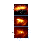
Figure 1: Images of our H and K-band mosaics from Keck/NIRC along with an extinction map derived from the molecular column density data of Goldsmith, Bergin, & Lis (1997). The pixel size of the infrared mosaics is 0.15$"$ and the angular resolution of the extinction map is 50$"$. Contours in the extinction map begin at A_V = 5 mag and are spaced at $\Delta$A_V = 10 mag intervals.

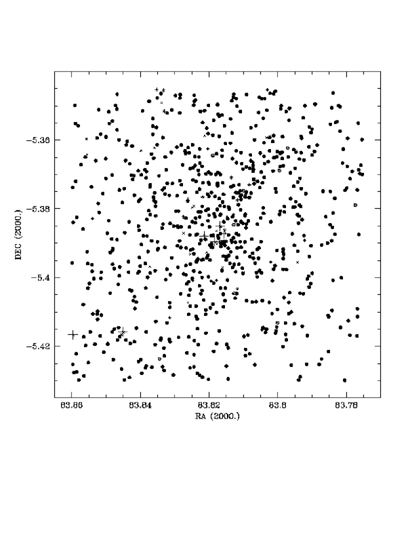
Figure 2: Spatial distribution of ONC stars within our NIRC mosaics. The $x$’s indicate stars whose photometry we could not derive, $x$’s surrounded by open circles indicate stars with photometry at K but not H, $\ast$’s indicate stars with photometry at H but not K, and filled circles indicate stars with photometry at both K and H. Large $+$ signs indicate the optically brightest stars, for orientation.

As the images were placed in the mosaic, the sky background was adjusted by an additive constant to match the background in the surrounding frames. The relative intensity offsets were determined by fitting a gaussian to the difference in image intensity in the overlap region between neighboring frames. As with the positional offsets, the sky offsets for all frames were determined simultaneously using a linear least-squares fit to all the overlap regions. We were unable to obtain an acceptable solution over the entire mosaic for the sky offsets at Z-band. Thus our Z-band photometry is derived from the individual frames and is not as deep as it would be if derived from a co-added mosaic. The Z-band data and supplemental calibration information are presented in a separate paper. The H- and K-band mosaics are shown in Figure 1 along with an extinction map which is described in section 5.2. Figure 2 shows the spatial distribution of stars in our sample, whose identification and photometry we describe next. Table 1 contains the coordinates and HK photometry.

4 Mosaic Analysis

4.1 Identification of Point Sources

Point sources were identified on the K-band mosaic using DAOFIND in IRAF with a 7$\sigma$ threshold. The initial source list was hand-edited to remove nebular knots, multiple listings of bright stars, diffraction spikes, edge effects, etc. We then examined contour plots of each point source to look for extended or double-peaked structure, and added any newly found sources. The final source list consists of 778 stellar point sources over the 5.1^′x5.1^′ field.

4.2 Aperture and Point-Spread Function Fitting Photometry

Aperture photometry was derived using PHOT with a 6 pixel radius aperture and a sky annulus extending radially from 7-12 pixels; contribution from the sky was determined from the mode of these values. The small aperture and the close sky annulus were necessitated mainly by the spatially variable background from the Orion Nebula, and to a lesser extent by the high source density. Aperture corrections were needed in order to correct from the 6 pixel radius used to measure the data to the 20 pixel radius used to measure the standard stars. The size of the aperture correction is directly related to the size (e.g. full-width-half-maximum; FWHM) of the point source. In our image mosaics, however, the point-spread-function (PSF) undergoes large and non-systematic spatial variations due to random wandering in time of the seeing compared to the 0.15$"$ platescale, and to a systematic gradient in airmass. We derived an empirical calibration between the aperture correction and the image FWHM, as follows.

First, recall that each stellar image in our final mosaic is synthesized from several (ideally four) separate observations of the star. Each of these observations may have a different PSF size. We verified that the PSFs of point sources in the final mosaic indeed have the mean value of the PSFs and the mean value of photometry through a fixed aperture size, characterizing the individual images from which they were created. In order to determine the appropriate aperture corrections for photometry from the mosaiced data, we therefore need only measure each of the PSFs in the final mosaic and apply a correlation between PSF and aperture corrections.

We measured the size of each stellar PSF using a variety of IRAF tasks – IMEXAMINE, RADPROF, and FITSPSF. From the 40 most isolated K $<$ 13 mag stars in the mosaic we found the tightest correlation (error in slope $<$ 0.01 mag) to be between the aperture correction and the “enclosed” gaussian fit FWHM of the IMEXAMINE task. In cases where this primary FWHM – aperture correction correlation could not be applied (e.g. failure of the gaussian fit to converge due to crowding and/or high nebulosity) we used secondary correlations. The FWHM values of $>$90% of the stars are between 3-5 pixels at K-band and between 4.5-6.5 pixels at H-band. The full range of the aperture corrections at K is from $\sim$ -0.10 mag to -0.60 mag with a mean value of -0.350 mag and at H is from $\sim$ -0.25 to -0.55 mag with a mean value of -0.325 mag. Variable aperture corrections are less of a problem at H compared to K since the overall size of the stellar images is larger which acts to decrease the percentage of PSF change as the seeing and airmass vary. Despite the complicated nature of our process for applying aperture corrections, we believe it is the proper one based on significant improvement in correlations between our NIRC photometry and previous photometry (described below). We did attempt to correlate aperture corrections with a measure of the difference in width between each stellar image and a PSF constructed from the data itself (the “sharpness” parameter of the PEAK task). But the correlation was too loose to be useful.

The point-spread-function was constructed using the PSF task and 30 stars distributed over the outer, less crowded, regions of our mosaics and having FWHM values distributed like the data as a whole. Accurate characterization of the noise in the mosaiced images was done so as to achieve the best possible fits of the point-spread-function to the stellar sources. In practice, this means adding a constant to the mosaics such that their standard deviation equals the sky counts plus the square of the effective read noise. A moffat function with $\beta$=1.5 gave the best residuals among the moffat, lorentzian, gaussian, and penny functions. As just discussed, the point-spread-function varies across our image due to seeing fluctuations and airmass changes. Because the variations are random and not smooth, we can not model them in any useful way and we are forced to fit the same point-spread-function to every star. The constructed point-spread-function was fit using the PEAK task with a fitting radius equivalent to twice the average FWHM. Both positional re-centering and sky re-calculation were permitted. Unfortunately, the resultant photometry was strongly influenced by which star was chosen as the first in constructing the PSF.

Comparisons between the aperture photometry and the point-spread-function fitting photometry are generally poor, due to the varying PSF. We have decided to use in our analysis the results from aperture photometry calibrated as described above. Our final photometry list was hand-edited to remove the measurements in cases of contamination from bright stars and/or overlapping apertures (44 stars) or nonlinearity (36 stars).

4.3 Integrity of Photometry

In this section we discuss the internal errors of our photometry and the comparison of our photometry to previous work.

Figure 3 shows the run of photometric error with magnitude and color. These internal errors are those produced by the PHOT routine in IRAF and simply reflect photon statistics of the source and sky determination in the fully processed images; they do not include other errors such as those in the zero point. At K-band, 75% of the stars in our source list have errors $<$0.02 mag, 90% have errors $<$0.05 mag, and 97% have errors $<$0.1 mag. At H-band, 69% of the stars in our source list have errors $<$0.02 mag, 85% have errors $<$0.05 mag, and 91% have errors $<$0.1 mag. For the PSF fitting photometry the percentages of stars with internal errors of the magnitudes given above were all down by 5 to 45 points, with the worst results at K-band. This is due to the generally poor fit of any single point-spread-function to all stellar images in the mosaic and part of our justification for rejecting the PSF photometry.

Figure  4 shows the comparison of our photometry to photometry from the 2MASS survey. Although the scatter is large ($\sim$0.2 mag) for the full sample of stars in common, it drops to $<$0.1 mag when only spatially well-isolated stars are considered (filled circles). Many of the largest deviations ($>$1 mag) are found in crowded regions where our photometry is always fainter than the 2MASS photometry, presumably due to our higher spatial resolution which permits better source separation and better sky determination. Nonetheless, there are also well-isolated stars with rather large differences in the photometry. Note, for example, the star at K_NIRC=10.3, K_NIRC-K_2MASS=-0.8. This is a very bright, very well-isolated star whose photometry differs by almost 1 mag at K between our NIRC data, the 2MASS data, our previous photometry with SQIID/NICMASS (Hillenbrand et al. 1998), and that published by Ali & DePoy (1995) and Hyland, Allen, & Bailey (1993; as reported by Samuel 1993). Incidentally, this star (JW 737) is a 4.5 mag variable at I-band (W. Herbst, private communication). We have no choice but to interpret cases such as this as examples of real infrared photometric variability. Variability may well be the cause of much of the spread along the ordinate in Figure 4. Indeed, we have strong evidence from Figure 18 (discussed in the Appendix) that short-term variations of order 0.1 mag are present in at least some stars in the Orion A molecular cloud. Comparisons between our NIRC photometry and that presented in Hillenbrand et al. (1998), and between 2MASS and Hillenbrand et al. (1998), show somewhat larger scatter in the magnitudes but similar scatter in the colors.

In summary, we believe that our photometry for bright, isolated stars is within $<$0.1 mag of that determined by others. Much of this scatter may be attributed to photometric variability, although some role is probably played by the variable PSF which plagued our photometry extraction. We note that our careful attention to aperture corrections improved considerably the correlations between our NIRC results, our previously published data, and the 2MASS survey. Based on the comparisons in Figure 4, however, for the analysis presented below we conservatively assume minimum K magnitude errors of $0.09/\sqrt{2}=0.06$ mag and minimum H-K color errors of $0.18/\sqrt{2}=0.13$ for all stars in our sample. The $\sqrt{2}$ factor implies that we ascribe equal errors to our data and to 2MASS data even though the formal 2MASS errors are much larger than the formal NIRC errors for these relatively bright stars.

4.4 Artificial Star Experiments

We determined the completeness of our point source list and the completeness of our photometry using results from extensive experimentation with artificial stars. First, fake source lists were generated by randomly distributing 300 stars over the $\sim$2080 $\times$ 2080 pixels² in our mosaics, with the caveat that no star be placed within 3 pixels of a known star or within 30 pixels of the edge of the frame. Next, stars with the point-spread-function derived as described above were added to the image at these 300 locations using ADDSTAR. The enhanced image was then run through the DAOFIND, PHOT, and PEAK tasks in a manner identical to that used to extract photometry from the unaltered data. A separate artificial star test was conducted for every 0.25 magnitude interval in the range 14-18.5 mag. Our results for finding fake stellar point sources are somewhat different from our results for photometering fake stellar point sources.

The DAOFIND results are that for a detection threshold of 20$\sigma$, we can identify fake stellar point sources in our images at the 90% completeness level down to K = 16.8 mag and at the 20% completeness level down to K = 17 mag. For a detection threshold of 7$\sigma$, we can identify fake stellar point sources at the 90% completeness level down to K = 17.7 mag and at the 20% completeness level down to K = 18.2 mag.

The DAOPHOT results are presented in Tables 2 and  3. We assess both the internal errors, the formal uncertainties in the output magnitudes, and the external errors, the differences between the input and the recovered magnitudes, as a function of magnitude and also radial position in the cluster. The strong and variable nebular background in combination with extreme point source crowding makes these experiments somewhat more difficult to interpret than in the usual case. Nevertheless, we conclude based on internal error estimates (Table  2) that at the limit of our ability to detect 90% of the stellar point sources (K = 16.8 mag for the 20$\sigma$ threshold which produces 94% of the stars in our source list), we are able to do photometry accurate to 0.02 mag for 15% of them, 0.05 mag for 68% of them, and 0.1 mag for 85% of them. For brighter stars the internal error estimates are lower. For fainter stars, at the K = 17.7 mag limit 7$\sigma$ detection threshold, the photometry is accurate to 0.02 mag for 0% of the sources, to 0.05 mag for 19% of them, and 0.1 mag for 59% of them. However, based on the external errors (Table  3), we seem perfectly capable of recovering the input stellar magnitudes to within a few percent down to K$\approx$17.5 mag. The numbers listed in each column of this table are the median offsets between input and output magnitudes, and also the standard deviations. Of note is that any bias in our photometry, when it appears at a moderately important level for stars K $<$ 17.5 mag, is such that the MEDIAN offset is positive, meaning that we seem to measure the star as slightly fainter than it really is, probably through over-subtraction of background. By contrast, the MEAN offsets are positive (meaning that we measure the star as being too bright), but we note that the MEAN values are dominated by just a few data points with special problems such as proximity to very bright stars; hence we prefer to quote MEDIAN offsets.

In conclusion, based on artificial star experiments we adopt a conservative K = 17.5 mag as the completeness limit for source detection. The 75% completeness limits for photometry accurate to 10% are K = 17.3 mag and H = 17.4 mag while the 50% numbers for photometry accurate to 10% are K = 18.0 mag and H = 18.1 mag. These numbers are averaged over the 5.1^′ x 5.1^′ field and mask the systematic gradient with radius caused by variable source crowding and nebular strength. We estimate that we have determined the completeness to an accuracy of a few tenths of a magnitude only, due in part to the radial gradient and in part to the spatially variable PSF. Note that we found our ability to reproduce the magnitudes assigned to fake stars in the input stage varied significantly with the parameters given to the PHOT, PSF, and PEAK tasks in IRAF. The parameters producing the most accurate results in the artifical star experiments were those then used to extract the real source photometry as described previously.

4.5 Astrometry

Our astrometry for the NIRC mosaics is referenced to the 2MASS database, which in turn is referenced to the ACT catalog. The nominal 1$\sigma$ 2MASS position error for bright, isolated sources is $\sim$ 0.1$"$ in each of right ascension and declination. An edited list of $\sim$230 stars in common between 2MASS and our Table 1 was used to derive the final astrometric solution, producing a platescale of 0.152$"$/pixel and a total r.m.s. error in the positions of 0.10$"$.

We note that the current astrometric system is shifted by about +1.5$"$ in right ascension and -0.3$"$ in declination compared to that presented by us previously. In an optical study of stars located within $\sim$20’ of the ONC core, Hillenbrand (1997) derived astrometry using the HST Guide Star Catalog (Lasker et al. 1988) which is known to suffer some inaccuracies in this region of the sky. We have found that our previous astrometric solution is offset to the west and to the south compared to other studies of the ONC (e.g. Jones & Walker 1988; McCaughrean & Stauffer 1994; Prosser et al. 1994; Ali & DePoy 1995; O’Dell & Wong 1996) but by various amounts as several of these studies have their own astrometric inaccuracies. The Jones & Walker positions and the McCaughrean & Stauffer positions are each internally consistent, although offset from one another. The McCaughrean & Stauffer astrometry matches our 2MASS-referenced astrometry. The HST positions of Prosser et al. and of O’Dell & Wong, however, are not internally consistent and suffer random excursions of about 1$"$ which were propogated into the Hillenbrand (1997) database. Likewise, the coordinates of Ali & DePoy suffer large random errors, of order 1.5-2$"$. Furthermore, approximately 1/2 of the sources supposedly located within our survey area as listed by Ali & DePoy simply do not exist in our higher resolution data; we do not discuss this catalog further. In summary, we believe that the positions quoted in Table 1 are both internally consistent and properly referenced to the ACT reference frame.

4.6 Properties of Final Source List

A fundamental result of this paper is a list of coordinates and available HK photometry for 778 stars in the inner 5.1^′ x 5.1^′ of the ONC. A total of 687 stars have measurements at both H and K, with 647 stars having errors $<$0.15 mag in both H and K. These data are presented in Table 1 along with cross-identifications to previously published optical and infrared source lists.

In the optical (Optical ID column), Jones & Walker (1988) numbers are listed with first priority, then Parenago (1954), Prosser et al. (1994), Hillenbrand et al (1997), and finally O’Dell & Wong (1996) if no other designation exists. Several of the previously cataloged optical stars appear not to be real sources based on their absence in our NIRC images. Another, although unlikely, possibility is that these are large-amplitude variables which have faded to K$<$17.5 mag. As listed in Hillenbrand (1997) these are 459 and 699 (Jones & Walker sources), 3071 and 3089 (Hillenbrand sources), and 9081 and 9326 (Prosser et al. sources). One other object, 3083, is the head of a teardrop-shaped “proplyd” identified from high-resolution HST images; we have left this spatially extended source in our photometry list along with several other “proplyds” which may not be point sources (e.g. OW-114-426, also extended in our images and clearly seen in silhouette in the Z-band data). In the infrared (Alternate Infrared ID column) McCaughrean & Stauffer numbers are given; we recover all stars from that survey except for a few close pairs – MS-86 is a close companion to P-1889, MS-65 is a close companion to P-1891 ($\Theta^{1}$C Ori), and MS-75 and MS-77 appear as a single source in our images. Finally, $\sim$250 of the sources with K$<$14.5 mag in Table 1 are also listed as point sources by 2MASS.

In summary, of the 778 stars in Table 1, $\sim 350$ are previously known from optical studies conducted to varying survey depths while $\sim 430$ are more heavily “embedded” in molecular cloud and/or circumstellar material. Of the embedded sources, approximately $\sim 125$ were previously catalogued (McCaughrean & Stauffer over the inner 1.4’ x 1.4’; Downes et al. 1981 and Rieke, Low, and Kleinmann 1973 in the BN/KL region) and all those K $<$ 13.5 mag over the full area of the current NIRC survey were found in previous studies at lower spatial resolution and lower sensitivity (e.g. Hillenbrand et al. 1998). There are $\sim$175 sources newly catalogued here. Nearly all of these do appear in images available from McCaughrean or the NAOJ / Subaru Telescope first light press release.

In deriving the ONC mass function, we have edited down the list of 778 in Table 1 to remove those with one or more of the following features: 1) no photometry at either K or H (21 sources); 2) photometry at K or H only, but not both (32 sources); 3) photometry given only as lower or upper limits at either K or H (38 sources); 4) photometry with internal errors $>$0.5 mag at either K or H (14 sources); and 5) brighter counterparts in close pairs where we can not derive photometry for the fainter counterpart because of contamination by the brighter one (15 sources). This last criteria was imposed so that the edited source listed would not be biased in any way against fainter, presumably lower mass, objects. The number of stars remaining for our derivation of the ONC stellar/sub-stellar mass function is 658.

5 Basic Results

5.1 The K Histogram and K–(K-H) Color-magnitude Diagram

In Figure  5 we present the histogram of K magnitudes for all objects with measurable photometry over our 5.1^′ x 5.1^′ field. Consistent with previous near-infrared studies of the ONC (McCaughrean et al 1995; Ali & DePoy 1995; Lada et al. 1996) we find that the K magnitude histogram rises to a peak around K = 12-12.5 mag and then declines. The minor peak at K$\approx$14.5 mag is also seen in Figure 2 of McCaughrean et al. (1995). The hatched portion of the Figure shows the sample remaining after removing stars without suitable photometry at both H and K according to the criteria listed above. This sample is not substantially different from the unhatched distribution representing the full photometric database.

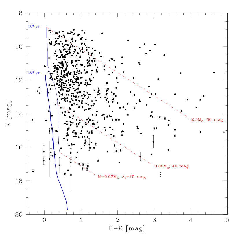
Figure 6: K vs H-K diagram for stars photometered with NIRC. Also shown is the 100 Myr isochrone (equivalent to the zero-age main sequence for masses M$>$0.35 M_⊙) and the 1 Myr pre-main sequence isochrone from D’Antona & Mazzitelli (1997, 1998) translated into this color-magnitude plane (solid lines). Reddening vectors (dashed lines) originate from the 1 Myr isochrone at masses of 2.5 M_⊙, 0.08 M_⊙, and 0.02 M_⊙. We believe that the source detection is 90% complete at the 7$\sigma$ theshold to K$>$17.5 mag. Internal errors in the K magnitudes are indicated; errors in the H-K color are larger than those in K band alone. The limit for 10% photometry occurs at K$\approx$17.3 mag and H$\approx$17.4 mag.

The K–(H-K) diagram for all stars with both H and K photometry from this study is presented in Figure 6. The 100 Myr isochrone (equivalent to the zero-age main sequence for masses M$>$0.35 M_⊙) and the 1 Myr pre-main sequence isochrone from D’Antona & Mazzitelli (1997, 1998), translated into this color-magnitude plane as described in section 6.1.3, are shown. Reddening vectors originating from the 1 Myr isochrone at masses of 2.5 M_⊙, 0.08 M_⊙, and 0.02 M_⊙ are indicated. Considering only stellar photospheres for the moment, our data are sensitive to all objects (stars and brown dwarfs) with ages $\sim$1 Myr and masses M$>$0.02 M_⊙ seen through values of extinction A${}_{V}<$ 10 mag. The observed colors of most of the objects are substantially redder than the expectations from pre-main sequence isochrones, a fact which can be attributed to a combination of extinction and excess near-infrared emission due to a circumstellar disk as discussed in section 6.2. Nevertheless, several tens of reddened objects located below the hydrogen burning limit at 0.08 M_⊙ are present. Most of these are probable young brown dwarfs, although some may be field stars.

5.2 Field Star Contamination

Our images and the resulting K-magnitude histogram and K–(H-K) color-magnitude diagram contain both ONC cluster members and unrelated field stars. Since H- and K-band photometry alone can not distinguish between cluster members and nonmembers, we assessed contamination to the star counts from field stars using a modified version the Galactic star count model of Wainscoat et al. (1992). While the nominal Wainscoat et al. model includes a smooth Galactic extinction distribution, the line of sight toward the ONC contains a substantial and spatially variable extinction component from the Orion molecular cloud, as was shown in Figure 1c. This extinction map was generated from the C¹⁸O column density data of Goldsmith, Bergin, & Lis (1997) by assuming a C¹⁸O/H₂ abundance of $1.7\times 10^{-7}$ (Frerking, Langer, & Wilson 1982) and that an H₂ column density of 10²¹ cm^-2 corresponds to 1 magnitude of visual extinction (Bohlin, Savage, & Drake 1978). The visual extinction peaks along the western part of the inner ONC with a maximum value A_V = 75 mag, and falls off sharply to the east to a minimum value of A_V = 3 mag at the edge of our NIRC map. Obviously the contribution from background field stars to the observed star counts will vary substantially across the ONC, in inverse relation to this extinction distribution. The number and near-infrared magnitudes and colors of expected field stars were obtained by convolving this extinction map with the nominal Wainscoat et al. star count model, although the additional extinction from the Orion molecular cloud was added only to the background field star population.

The distribution of K magnitudes for the field stars was shown in Figure 5 (dashed curves), both before and after convolution with the molecular extinction map. With addition of the proper amount of extinction at the distance of the Orion cloud, the numbers predicted for foreground/background contamination in our data are reduced to 0.08 stars arcmin^-2 at K$<$13 mag (from 0.17 stars arcmin^-2), 0.27 stars arcmin^-2 at K$<$15 mag (from 0.76 stars arcmin^-2), and 1.54 stars arcmin^-2 at K$<$18 mag (from 3.41 stars arcmin^-2). The total number of stars predicted to contaminate our NIRC photometry down to the K completeness limit (17.5 mag) is 34 (with 43 down to K=18 mag), representing a small but non-negligible 5% of our survey sample.

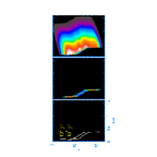
Figure 11: Model K–(H-K) diagrams for various assumptions about the age and near-infrared excess distributions. The mass function is log-uniform between 0.017 and 3.0 M_⊙. The left panel shows the K–(H-K) distribution of two single-aged populations at 10⁵ and 10⁶ years, with no near-infrared excess. The middle panel shows a population distributed log-uniform in age between 10⁵ and 10⁶ years, as we adopt for the ONC (see Figure 8), and again with no near-infrared excess. The right panel shows the same log-uniform age distribution but now includes the near-infrared excess distribution adopted for the ONC (see Figure 9).

In Figure 7 we compare the ONC data (panel a) to the model field star population (panel b). For the data we have used the edit source list of 658 stars discussed above and for the field stars we have convolved the model with the photometric errors as a function of magnitude characterizing the NIRC photometry. A Hess diagram format was adopted, where individual points have been smoothed with an elliptical gaussian corresponding to the photometric uncertainties. This Figure highlights the large concentration of observed stars with K $\approx$ 12 and H-K $\approx$ 0.5, and affirms that the the density of stars in the K–(H-K) diagram is dominated by ONC cluster members at all but the faintest mangitudes. To derive the K–(H-K) distribution of stars actually associated with the ONC we subtracted panel (b) from panel (a), as shown in Figure 11a.

6 Analysis: The ONC Mass Spectrum Across the Hydrogen-Burning Limit

The goal of this study is to translate the information contained in the K–(H-K) diagram shown in discrete format in Figure 6 and in Hess format in Figure 7a, into information on the stellar/sub-stellar mass function. This is not a trivial transformation since the location of a young star in the K–(H-K) diagram depends on four parameters: stellar mass, stellar age, presence and properties (e.g. accretion rate) of a circumstellar disk, and extinction. A moderately bright, red object, for example, while usually thought of as a massive star seen through large extinction, can also be a much lower mass star with a large near-infrared excess and significantly lower extinction. Indeed, bright red objects can be reproduced by a number of combinations of stellar mass, stellar age, near-infrared excess, and foreground extinction. Faint, blue stars on the other hand, can come only from the lower masses, older ages, smaller near-infrared excesses, and lower extinctions. The distribution of data points across the K–(H-K) diagram is dictated by the interaction occuring for each star in the cluster of these four primary physical parameters.

Photometry alone can not be used to deconvolve the age, near-infrared excess, and extinction distributions to obtain uniquely the mass of the object. Such an effort would require spectroscopic observations for the entire cluster population, which currently do not exist. Therefore, a variety of techniques making various assumptions about these parameters have been developed in order to constrain the initial mass function. The most common of these approaches is to determine if the peak and the width of a K-band histogram are consistent with both an assumed initial mass function and a “reasonable” stellar age distribution (Zinnecker & McCaughrean 1991). One drawback to this approach is that the information inherent to multi-band photometry often is not used to constrain other two parameters: the extinction and the near-infrared excess properties of the individual stars. Other approaches attempt to use multi-band photometry to de-redden individual stars and to consider the effects of near-infrared excess in estimating individual stellar masses from a single mean mass-luminosity relationship (e.g. Meyer 1996). A drawback of this approach is that it assumes that the near-infrared excess at the shortest wavelength is negligible, and that the mean age of the entire cluster is a good approximation for each individual member of the cluster.

Here, we describe a new method for deriving the stellar mass function that acknowledges the existence a distribution of stellar ages, near-infrared excesses, and extinction values in star-forming regions. We use these distributions to determine the probability a star could be a certain mass based on its location in the K–(H-K) diagram, as opposed to estimating unique masses for individual stars. The advantages to this approach are that we use all the photometric information available, we make no a priori assumptions about the shape of the mass function, and we incorporate the inherent photometric uncertainties. Before describing our method for inverting the observed K–(H-K) diagram to derive the mass function, we first establish the stellar age and near-infrared excess distribitions appropriate for the ONC needed for our analysis.

6.1 Assumptions

6.1.1 Stellar Ages

Hillenbrand (1997) used the D’Antona & Mazzitelli (1994) tracks to find a mean age for low-mass optically visible ONC stars of 0.8 Myr with an age spread of up to 2 Myr. We show in Figure 8 the age distribution derived using the more recent D’Antona & Mazzitelli (1997, 1998) calculations and updated spectral-type – temperature – color – bolometric correction relations, described below. This Figure includes only stars within the area of our NIRC survey. Hillenbrand (1997) discussed the presence of a radial gradient in the stellar ages where the mean age for stars in the inner ONC is slightly younger (by 0.25 dex or so) than the mean age for the ensemble ONC. This trend is also present using the updated theory and observational-to-theoretical transformations. Based on Figure 8, we adopt in what follows an age distribution which is uniform in log between 10⁵ and 10⁶ yr; we also consider a distribution which is uniform in log between 3x10⁴ and 3x10⁶ yr with little difference in the results.

6.1.2 Near-Infrared Excess

We quantify the near-infrared excess using the H-K color excess, defined as $\Delta(H-K)=(H-K)_{observed}-(H-K)_{reddening}-(H-K)_{photosphere}$. Spectroscopic and photometric data presented in Hillenbrand (1997) and Hillenbrand et al. (1998) allow us to compute this quantify for those optically visible stars within the area of our NIRC mosaic. $(H-K)_{observed}$ is the tabulated color. $(H-K)_{reddening}=0.065~{}A_{V}$ where $A_{V}$ is derived from the spectral type and observed V-I color in comparison to expected V-I color and $A_{V}=2.56~{}E(V-I)$. $(H-K)_{photosphere}$ comes from the relation between temperature and intrinsic H-K color described below. A histogram of the derived H-K excesses is shown in the top panel of Figure 9. We find that the observed near-infrared excesses can be well represented by a half-gaussian with a dispersion $\sigma$=0.4 mag, as shown by the solid line. In practice, we truncate the gaussian at $\Delta$(H-K) = 1 mag, which is the maximum H-K excess observed in the inner ONC. Hillenbrand et al. (1998) discussed the presence of a radial gradient in ONC near-infrared excess values with the mean near-infrared excess (measured as $\Delta(I-K)$ instead of the $\Delta(H-K)$ used here) larger for stars in the inner ONC than for the ensemble ONC. We emphasize, therefore, that the H-K excess distribution presented in Figure 9 is known to be accurate for the inner ONC only, although we note that the distributions similarly calculated for young stellar populations in Taurus-Auriga, IC348, L1641, NGC2264, NGC2024, MonR2, and Chamaeleon using literature data (see description of samples and procedure in Hillenbrand & Meyer, 2000) are generally similar in form although slightly narrower in width.

In addition to the H-K excess, we must estimate the excess at K band alone in order to properly model the K–(H-K) diagram. Since the K magnitude excess is more difficult to compute accurately than the H-K color excess, we have used the K excesses tabulated for pre-main sequence stars in the Taurus molecular cloud by Strom et al. (1989) and the H-K excesses calculated as above using data from Kenyon & Hartmann (1995) to establish an empirical relation between these quantities. The bottom panel in Figure 9 shows the correlation between the K and H-K excess derived for stars in Taurus, which can be represented by a linear fit of $\Delta$K = 1.785 $\times$ $\Delta$(H-K) + 0.134 with a scatter of $\pm$ 0.25 mag. We assume that this relationship also holds for stars in the ONC.

6.1.3 Translations from Theoretical to Observational Quantities

The final step before we can create models of the K–(H-K) diagram is conversion of theoretical pre-main sequence evolution into the observational plane. We use the theoretical description of luminosity and effective temperature evolution with mass according to D’Antona & Mazzitelli (1997,1998). These tracks are the only set available which cover the full range of masses sampled by our data, at the numerical resolution needed. We note, however, that the most recently circulated calculations of pre-main sequence evolution by various groups (D’Antona & Mazzitelli; Burrows et al.; Barraffe et al.;) do seem to be converging in the ranges where they overlap. Nevertheless, we must note that the details of our results likely are sensitive to the set of tracks/isochrones we have adopted.

We have transformed the D’Antona & Mazzitelli (1997,1998) calculations of L/L_⊙ and T_eff/K into K magnitude and H-K color using Chebyshev fits (Press et al. 1989) to bolometric correction, V-I color, I-K color, and H-K color vs effective temperature. For the mass range of interest in this paper we have taken the empirical data on bolometric corrections from Bessell (1991), Bessell & Brett (1988), and Tinney, Mould, & Reid (1993); on colors from Bessell & Brett (1988), Bessell (1991), Bessell (1995), Kirkpatrick & McCarthy (1994), and Leggett, Allard, and Hauschildt(1998); and on effective temperatures from Cohen & Kuhi (1979) – effectively Bessell (1991) – Wilking, Greene, & Meyer (1999), and Reid et al. (1999).

Note that these relationships are somewhat different than those used in Hillenbrand (1997, 1998). We have now shifted the temperature scale cooler and the bolometric corrections slightly smaller at the latest spectral types, in keeping with current consensus that was not well-established at the time of our earlier work. The combination of updated tracks and updated transformations between observations and theory have caused a shift in our interpretation of the optical data presented by Hillenbrand (1997). As we show in Figure 10, instead of a mass function that rises to a peak, flattens, and shows evidence for a turnover (bottom panel), the same data now appear to suggest a mass function for the greater ONC which continue to rise to the mass limit of our previous survey (top panel).

Finally, in the current analysis, we use the Cohen et al. (1981) reddening vector, A_K=0.090 A_V and A_H=0.155 A_V, and assume the Genzel et al. (1981) distance of 480$\pm$80 pc to the ONC (distance modulus = 8.41 mag).

6.2 A Model for the Distribution of Stars in the K–(H-K) Diagram

Given the above assumptions concerning the age and near-infrared excess distributions for the inner ONC, and the translation of theoretical tracks/isochrones into the K–(H-K) plane, we are now in a position to construct model K–(H-K) diagrams. In Figure 11 we illustrate the effects of various age and near-infrared excess distributions on the appearance of the K–(H-K) diagram. Panel (a) shows discrete isochrones from the calculations of D’Antona & Mazzitelli (1997, 1998) for ages of 10⁵ and 10⁶ year; panel (b) shows a sample of stars uniformly distributed in log-mass between 0.02-3.0 M_⊙ and uniformly distributed in log age between 10⁵ and 10⁶ year; panel (c) shows the same mass and age distribution of (b) but now includes the near-infrared excess distribution parameterized in Figure 9. No extinction is included in these panels. Note that in the case of a uniform age distribution (panel b), the K–(H-K) diagram is not uniformly populated between the limiting isochrones. As originally shown by Zinnecker & McCaughrean (1991) in an analysis of K band histograms, the onset of deuterium burning occurs at different times for different masses, leading to distinctive peaks in the magnitude and color-magnitude distribution for pre-main sequence stars. These peaks become less distinctive when a near-infrared distribution is added (as shown in panel c) and even less distinctive when extinction is added (as shown next).

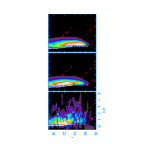
Figure 12: Simulations of the K–(H-K) diagram using the age distribution assumed from Figure 8, the near-infrared excess distribution assumed from Figure 9, and an extinction distribution which is uniform in the interval A_V=0-5 mag. The middle panel shows the log-normal form of the Miller-Scalo mass function while the right panel shows a shallow power law mass function (N(log M) $\propto$ M^-0.35). Our data are shown in the left panel, which is the subtraction of the field star model in Figure 7b from the observations in Figure 7a. The models suggest that a falling mass function like that of Miller-Scalo better represents the peak in the observed ONC star counts than does an increasing mass function like the shallow power-law. Although there appear to be some more highly extincted stars in the data than in these models, broadening the A_V distribution in the models dilutes the peak; this suggests that the bulk of the ONC stars are found at relatively low extinction, A${}_{V}<$ 10 mag.

We incorporate elements of Figure 11 to show in Figure 12 (note the change in scale, now set to match the range of our data) two model K–(H-K) diagrams in comparison to our NIRC observations. Panel (a) shows the ONC data of Figure 7a with the field star model of Figure 7b subtracted. Panel (b) shows a stellar population distributed in mass according to the Miller-Scalo mass function and distributed in age between 10⁵-10⁶ yr log-uniform, then also having the near-infrared excess distribution parameterized in Figure 9 and seen through extinction uniformly distributed between A_V=0-5 mag. Panel (c) is the same as panel (b) except that the mass distribution is now a power-law function instead of a Miller-Scalo function. The salient difference between these two mass functions is that the Miller-Scalo function (N(log M) $\propto$ e${}^{-C1(logM-C2)^{2}}$; C=1.14, C2=-0.88 as in Miller & Scalo, 1979) slowly declines across the hydrogen burning limit as N(log M) $\propto$ M^0.37 if forced to a power-law, while the straight power-law function (N(log M) $\propto$ M^-0.35) slowly rises. In creating Figure 12 we have not attempted to reproduce the observations; we wish merely to illustrate the combined effects in the K–(H-K) diagram of different assumptions about the mass, age, near-infrared excess, and extinction distributions. Note in particular that there are many stars observed (panel a) through higher values of A_V than we have considered in the models (panels b and c). Nevertheless, if we accept that our assumptions about the age and near-infrared excess distributions (as derived from optically visible stars in exactly this region) are approximately correct, then we must conclude that a declining mass distribution such as the Miller-Scalo function is a much better match to the data than a rising power-law (or even a flat) function. We quantify these impressions in the following section.

6.3 Implementation and Tests

6.3.1 Calculating Mass Probability Distributions

How can the effects of stellar age, near-infrared excess, and extinction be disentangled to derive the mass function? As already discussed, the main difficulty is that more than one stellar mass can contribute power to any particular location in the K–(H-K) diagram through various combinations of these variables. Fortunately, however, the range of stellar masses that a given H-K,K data point could represent is constrained by the stellar age and near-infrared excess distributions, which for the inner ONC we are able to measure (Figures 8 and  9), and by the slope of the reddening vector.

In practice we calculate the stellar mass function as follows. We take as a starting point the observed K–(H-K) grid shown in Figure 12a. Recall that each star has been smeared out in this diagram by an elliptical gaussian corresponding to its photometric error; increasing the error even by a factor of 3 in each direction does not change the form of the distribution. We project every 0.01 mag wide pixel populated by data back along the reddening vector to establish which of the other pixels are crossed, and hence which combinations of unreddened K magnitudes and H-K colors the star or star-plus-disk system could have. Using a model K–(H-K) diagram, we keep track of the probability that a star of given mass can occupy that H-K,K combination given the assumed stellar age and near-infrared excess distributions. We sum the probabilities for all of the possible H-K,K combinations along the reddening vector, and then normalize to unity the integerated probability over all masses 0.02-3.0 M_⊙; i.e., the star must have have some mass within the considered range. By weighting the mass distribution derived for each pixel in Figure 12a by the relative density of observational data it represents, and summing the probability distribution for all pixels, we produce the cluster mass function. In a similar manner, we calculate probability distributions in A_V for each pixel, which we also density weight and sum to produce the cluster extinction distribution.

Examples of individual stellar mass probability distributions obtained by de-reddening a star in the K–(H-K) diagram are shown in Figure 13 for a representative set of K magnitudes and H-K colors. A K=15 mag relatively blue (H-K=0.5 mag) star is permitted to have a mass anywhere in the range $\sim$0.02-0.04 M_⊙ with a most likely value just above 0.02 M_⊙, while a K=15 mag much redder (H-K=3.0 mag) star has a broader range of permitted masses, $\sim$0.03-0.6 M_⊙ with a most likely value $\sim$0.2 M_⊙. Note the tails upward at the lower and upper mass extrema in the panels for K=16, H-K=0.5 and K=9, H-K=3.0, respectively. These are caused by our imposition of integrated probability equal to unity over the mass range contained in the theoretical grid; in reality such stars have some probability of coming from smaller and higher masses (respectively) than the 0.02-3.0 M_⊙ range considered here. The requirement of an integrated mass probability of unity means that the outer few bins of our resultant mass distribution may be unreliable.

Examples of individual extinction probability distributions are not shown since extinction is essentially the independent variable in our technique. Because we project each “star” back along the reddening vector and keep track of the stellar mass, stellar age, and near-infrared excess combinations that can conspire to produce that color-magnitude location, any given star can have any value of extinction ranging from a minimum of zero (in general, although it is not always true that there is a zero-extinction solution) to a maximum set by the case of de-reddening to the oldest considered age (i.e. bluest possible original location in the K–(H-K) diagram) and having no near-infrared excess. The result is that an extinction distribution which is uniform will be recovered using our methodology as an extinction distribution that has an extended tail induced by a combination of the age range and the near-infrared excess range considered in the de-reddening process.

6.3.2 Tests of Methodology

Before applying our newly developed methodology for deriving the stellar/sub-stellar mass function, we wish to test how accurately this method can recover a known mass function. For these tests we generated cluster models with various stellar mass, stellar age, near-infrared excess, and extinction distributions, and then attempted to recover the underlying mass function using the procedure described above. Figures 14 and  15 illustrate a sampling of the results. In general, we are fairly confident in our ability to recover the general form of the input mass distribution for masses 0.03 $<$ M/M_⊙ $<$ 1. Outside of these mass limits we suffer problems due to “edge effects” given the 0.02-3.0 M_⊙ range of the theoretical models we employ, and also due to saturation in our data at K $<$ 9 mag. In particular we note that in all cases we easily distinguish between mass functions that slowly fall across the hydrogen burning limit into the brown dwarf regime, as N(log M) $\propto$ M^0.37, and those that slowly rise, as N(log M) $\propto$ M^-0.35.

In Figure 14, we present test results where the stellar age and near-infrared excess distribution assumed in extracting the mass function from the K–(H-K) diagram is the same as the input cluster model. Thus these tests probe the success of the method when the cluster properties are accurately known a priori. Each of these models contain a log-uniform age distribution between 10⁵-10⁶ yr. The left panels are for models where the input mass function is Miller-Scalo while the right panels are for a power law of form N(log M) $\propto$ M^-0.35. The top panels are models with no extinction and no near-infrared excess; the middle panels include uniform extinction between A_V=0-5 mag; and the bottom panels include both uniform extinction and the near-infrared excess distribution parameterized in Figure 9. Note that the two bottom panels correspond to the cases shown in the K–(H-K) diagrams of Figure 12bc. Looking at the difference between the top and middle panels, addition of extinction to a model (surprisingly) helps our method to recover the input mass function. Looking at the difference between the middle and bottom panels, addition of near-infrared excess hurts slightly but only at the tails in mass. These test results illustrate that our method can never perfectly recover the input mass function as long as there is a spread of ages or of near-infrared excesses – even if these distributions are known. H- and K-band photometry alone can not uniquely determine the mass, age, near-infrared excess, and extinction which go into producing the observed color-magnitude location, and hence our method considers all possible combinations of these parameters. The result is imperfect; nevertheless, it seems clear from Figure 14 that we do reasonably well in recovering the general shape of the input mass function.

In Figure 15, we present test results where we deliberately choose an incorrect cluster age and/or near-infrared distribution to de-redden the K–(H-K) diagram. These tests probe how robust our procedure is in recovering the mass function when faced with uncertainties in characterizing the actual cluster properties. In each of these tests, the input cluster contains the same age distribution and near-infrared excess distribution that we assumed for the ONC. In addition, we added uniform extinction between A_V=0-5 mag. The left panels are tests results for the Miller-Scalo mass function, and the right panels for a power law mass function. The top three panels (left and right) show the effects of incorrect assumptions about the cluster age in the de-reddening process. Single-age assumptions give the worst results with two effects occurring. The first is a general shift of the recovered mass function towards higher masses as the age assumption is moved to older ages, due simply to the decrease in luminosity with age for a given mass star. The second effect is a “kinking” in the recovered mass function which is caused by considerable flattening of single isochrones in the 0.3-0.1 M_⊙ range compared to higher and lower masses in the K–(H-K) diagram. When a range of ages is assumed in the de-reddening, instead of just a single age, this effect is smeared out. Note that there is little difference between the panels which assume the correct age distribution, log-uniform between 10⁵ and 10⁶ yr, and the panels which assume a somewhat broader age distribution, log-uniform between 3x10⁴ and 3x10⁶ yr. The bottom panels (left and right) show the effects of an incorrect assumption about the near-infrared excess. When no infrared excess is allowed for in the de-reddening process too much power is given in the recovered mass function to higher masses relative to lower masses.

To summarize our test results, we find that we can recover the input mass function with some reasonableness in all cases where we know the correct stellar age and near-infrared excess distributions, and in most cases where we assume somewhat (but not grossly) incorrect representations for these distributions. The worst results are obtained when the cluster consists of a uniform age distribution, but a single age is assumed to derive the mass function. Since the spectroscopic data for the ONC indicate an age spread, this is in fact the least applicable case for this study. Based upon these test results, we expect that our procedure to recover the input mass function performs well over the mass range 0.03$<$M/M_⊙$<$1, and that it can distinguish between mass functions that slowly fall across the hydrogen burning limit, as N(log M) $\propto$ M^0.37, and those that slowly rise, as N(log M) $\propto$ M^-0.35.

6.4 Results on the ONC Stellar/Sub-stellar Mass Function

Using the procedure we have described and tested above, we present in Figure 16 the ONC mass function resulting from our best determinations of the appropriate stellar age (Figure 8) and near-infrared excess (Figure 9) distributions. Of the 658 stars with suitably good H and K photometry going in to this analysis, we recover 598 when we integrate over this mass function. The loss of $\sim$9% is due to color-magnitude diagram locations (spread by photometric errors; see Figure 7a) with no solution inside the bounds of the mass grid considered in this analysis given the assumed age and near-infrared excess distributions. Since bright massive stars can be detected through larger values of extinction than faint brown dwarfs, we also plot the mass function for only those objects meeting certain extinction criteria: first, only those with A${}_{V}<10$ mag, the highest extinction level to which 0.02 M_⊙ objects can be detected given the sensitivity limits of our survey, and second, only those with A${}_{V}<2.5$ mag, the extinction limit to which 0.1 M_⊙ objects could be detected in the optical spectroscopic survey by Hillenbrand (1997), to which we compare our infrared photometric results below. Of the total of 598 sources in the mass function of Figure 16 (open histogram), 67% have A${}_{V}<10$ mag while 28% have A${}_{V}<2.5$ mag.

As shown in Figure 16, the stellar/sub-stellar mass function in the ONC peaks near $\sim$ 0.15 M_⊙ and is clearly falling across the hydrogen burning limit into the brown dwarf regime – regardless of the adopted extinction limit, which affects the shape of the mass function only at the higher masses. We have investigated the robustness of Figure 16 for different plausible age ranges (e.g. log-uniform between 3x10⁴ and 3x10⁶ yr instead of between 1x10⁵ and 1x10⁶ yr), with and without a near-infrared excess distribution, and also with and without subtraction of field stars. The same basic conclusion is found. A power law fit to the declining inner ONC mass function for A${}_{V}<$ 10 mag between 0.03 M_⊙ and 0.2 M_⊙ has a slope of 0.57 $\pm$ 0.05 (in logarithmic units), where the uncertainties reflect only the residuals of the least squares fit to the data. Our best determination of the inner ONC mass function is inconsistent at the $>10\sigma$ level with a mass function that is flat or rising across the hydrogen burning limit.

According to the tests of our methodology (section 6.3.2), there are two ways to add power at low masses relative to higher masses and thus produce a less steeply declining or even flat slope across the hydrogen-burning limit: by making the cluster age much younger than we have assumed, and/or by making the near-infrared excesses much larger than we have assumed. We find neither of these options probable given the characteristics of the optically visible stars in the region, and hence we conclude that the inner ONC mass function is indeed declining. We have shown the accuracy to which our methodology recovers a known input mass function in Figure 14. Based on fits over the same 0.03-0.2 M_⊙ mass range we consider for the data, we conclude that our method recovers the correct slope of the input mass function to within $<$0.05. Combining this methodology error with the r.m.s. fitting error of $\pm$0.05 discussed above, we estimate the total error on the slope derived here for the ONC mass function across the hydrogen burning limit at $<$0.1. We offer the following two additional cautions to any interpreters of our results.

First, we emphasize that the detailed shape of the mass function derived from data is still subject to dependence on theoretical tracks and isochrones (D’Antona & Mazzitelli; 1997, 1998 in this case), and on the calibrations used in converting between effective temperature / luminosity and K–(H-K) color/magnitude (discussed in section 6.1.3).

Second, we emphasize that our derived mass function is valid only for the inner 0.71 pc $\times$ 0.71 pc of the ONC cluster, which extends at least 8-10 pc in length and 3-5 pc in width. Our conclusions may not apply to the ONC as a whole where some evidence for general mass segregation has been found by Hillenbrand (1997) and Hillenbrand & Hartmann (1998). In Figure 17 we compare the mass function derived here for the inner cluster using near-infrared photometry to that derived previously by us using optical photometry and spectroscopy. The histogram is the mass function of Figure 16 with an extinction limit of A${}_{V}<$ 2.5 mag, for consistency with the effective extinction limit of the optical data. Solid symbols represent the full dataset from Hillenbrand (1997) while open symbols represent only that portion of the data which are spatially coincident with the near-infrared photometry used to derive the histogram (i.e. the inner 0.35 pc or so). The same A${}_{V}<$ 2.5 mag imposed on the infrared data has also been imposed on the optical data. As noted in reference to Figure 10, the updated pre-main sequence tracks and the updated transformations between observational and theoretical quantities adopted in this paper have caused a shift in our interpretation of the data presented by Hillenbrand (1997). The large-scale ONC mass function (solid symbols) now appears to be rising to the limit of that survey. The inner ONC mass function (open symbols), however, appears to flatten below $\sim$0.3 M_⊙. This flattening is confirmed by the near-infrared photometric analysis presented here, and in fact is the beginning of a turnover in the mass function above the hydrogen burning limit and extending down to at least 30 M_Jupiter.

7 Discussion

Our analysis of the mass distribution in the inner ONC agrees with that of McCaughrean et al. (1995) in that there is “a substantial but not dominant population of young hot brown dwarfs” in the inner ONC. Although we do find $\sim$80 objects with masses in the range 0.02-0.08 M_⊙, the overall distribution of masses is inconsistent with a mass function that rises across the stellar/sub-stellar boundary. Instead, we find that the most likely form of the mass function in the inner ONC is one that peaks around 0.15 M_⊙ and then declines across the hydrogen-burning limit to the mass limit of our survey, 0.02 M_⊙. The best-fit power-law for the decline, N(log M) $\propto$ M^0.57, is steeper than that predicted by the log-normal representation of the Miller-Scalo initial mass function, N(log M) $\propto$ M^0.37 if forced to a power-law (see Figure 16).

How do our results compare to other determinations of the sub-stellar mass function? Thusfar there have been few actual measurements of the sub-stellar mass function which are not either lower limits or dominated by incompleteness corrections or small-number statistics. We can compare our results for the inner ONC only to those in the Pleiades (Bouvier et al. 1998; Festin 1998) and the solar neighborhood (Reid et al. 1999), and we find some differences. Converting the logarithmic units used thusfar in this paper (N(log M) $\propto$ M^Γ) to the linear units adopted by others (N(M) $\propto$ M^α) we find a mass function slope across the hydrogen-burning limit of $\alpha=\Gamma-1$ = -0.43. In the Pleiades, Bouvier et al. find $\alpha$ = -0.6 while Festin finds $\alpha$ in the range 0 to -1.0. In the solar neighborhood, Reid et al. find $\alpha$ in the range -1.0 to -2.0 with some preference for the former value. The methods used by these different authors for arriving at the slope of the mass function are very different, thus rendering somewhat difficult any interpretation of the comparison. Furthermore, it is not clear that the mass function in the center of a dense and violent star-forming environment should bear any similarity to the mass function in a lower-density, quiescent older cluster, or that either of these cluster mass functions should look anything like the well-mixed, much older local field star population. Nevertheless, if comparisons can be made, the inner ONC seems to have a shallower slope than that found in any other region where measurements have been made; recall as well that the inner ONC mass function appears shallower than the overall ONC mass function (see Figure 17).

8 Conclusions

We have introduced a new method for constraining the stellar/sub-stellar mass distribution for optically invisible stars in a star-forming region. A comparative review of the various techniques already in use for measuring mass functions in star-forming regions is presented by Meyer et al. (2000). These techniques range from studies of observed K-magnitude histograms (e.g. Muench et al. 2000), to discrete de-reddening of infrared color-magnitude diagrams (e.g. Comeron, Rieke, & Rieke 1996), to the assembly of photometric and spectroscopic data from which HR diagrams are created (e.g. Luhman & Rieke 1998). Our method is a variation on and an improvement to the discrete de-reddening of color-magnitude diagrams since we fully account for distributions in the relevant parameters instead of assuming a mean value for them. However, our method is not as good as a complete photometric - plus - spectroscopic survey since we produce only a mass probability distribution for each star, not a uniquely determined mass. Nonetheless, we believe that the statistical nature of our method does provide the most rigorously established constraint to date from photometry alone on the stellar mass function in a star-forming region.

We have used information from previous studies of optically visible stars in the ONC to derive plausible functional forms for the stellar age and the circumstellar near-infrared excess distributions in the innermost regions studied here. We assume that these distributions apply equally well to the optically invisible population. We find a mass function for the inner 0.71 pc x 0.71 pc of the ONC which rises to a peak around 0.15 M_⊙ and then declines across the stellar/sub-stellar boundary as N(log M) $\propto$ M^Γ with slope $\Gamma=0.57$. This measurement is of the primary star/sub-star mass function only, and should be adjusted by the (currently unknown) companion mass function in order to derive the “single star mass function,” if desired.

We find strong evidence that the shape of the mass function for this inner ONC region is different from that characterizing the ONC as a whole, in the sense that the flattening and turning over of the mass function occurs at higher mass in the inner region than in the overall ONC. In fact, the shape of mass function for the overall ONC is currently unconstrained across the stellar/sub-stellar boundary, and appears now based on the most recent theoretical tracks and conversions between the theory and observables used in this paper, to continue to rise to at least 0.12 M_⊙.

Appendix A The Infrared Variable 2MASSJ053448-050900 = AD95-1961

In this appendix we report on short timescale variability at infrared wavelengths of a star located approximately 15’ north-west of the ONC. Our observing procedure in constructing our 5.1’ x 5.1’ mosaic with NIRC was to scan across a row at constant declination, then move off to a sky position and obtain five measurements of the sky which were then averaged and subtracted from each frame in our ONC mosaic. We intentionally chose a sky field which included a relatively bright (K$\approx$ 14.0 mag) star in order to monitor the atmospheric extinction as part of our normal data acquisition. However, while our set of absolute standards from Persson et al. (1998) matched nominal NIRC zero points and nominal Mauna Kea extinction curves with airmass, our local standard exhibited significant flux variations (Figure 18). The amplitude of the variations is about 0.1 mag, and the timescale is less than the separation of our observations, about 10-12 minutes.

2MASSJ053448-050900 is also catalogued as AD95-1961 (Ali & DePoy 1995). This star has infrared fluxes of K=14.03 mag, H=14.43 mag, J=15.46 mag from the 2MASS survey and optical fluxes of I$\approx$17.5 mag, V$\approx$21.1 mag from our own unpublished CCD observations. These colors are consistent with those of low-mass ONC proper motion members.

The short-term photometric behavior of this relatively isolated and otherwise nondescript star located in the outer regions of the ONC may in fact be a general feature of all young stellar objects. Infrared monitoring studies of young clusters are needed in order to quantify the nature and constrain the causes of this variability.

Figure 3: Internal (IRAF) errors in photometry at H- and K-band, and in H-K color.

Figure 4: Comparison of NIRC and 2MASS photometry. Open circles represent all positional matches $<$ 1” between our NIRC sources and 2MASS sources while filled circles represent a set of relatively bright, isolated stars (those used to derive the aperture corrections). At K, the standard deviation per point about the mean is 0.19 mag for the full sample but 0.08 mag for the isolated stars. At H, the standard deviations are 0.22 mag and 0.09 mag for the full sample and for the isolated stars. In H-K, the values are 0.17 mag and 0.19 mag.

Figure 5: Distribution of K magnitudes for stars photometered with NIRC. The open histogram represent all stars with measured K magnitudes while the hatched histogram represents a reduced sampled of stars used in the mass function analysis. See text for explanation of the second sample. Short-dashed line represents the Galactic model of Wainscoat et al. (1992); long-dashed line represents the same model but reddened for stars located behind the cloud by the extinction map shown in Figure 1.

Figure 7: Hess format K–(H-K) diagram for our data (left panel) and an appropriately reddened field star model (right panel). To generate the contours for the observations, individual stars were smoothed by an elliptical gaussian corresponding to their photometric errors as described in the text. Similarly, the field star model was convolved with the typical photometric error as a function of magnitude. The white solid/dotted line is the 1 Myr pre-main sequence isochrone with the transition from a solid to dotted occuring at the hydrogen burning limit of 0.08 M${}_{o}dot$. The lowest mass represented by the isochrone is 0.017 M_⊙. The reddening vector for A${}_{V}<$ 50 mag is indicated by red dashed lines. The color stretch is identical for both panels, with the data plot containing 658 stars and the field star model containing 34 stars down K=17.5 and 43 stars down to K $<$ 18 mag. These figures demonstrate that field stars make a negligible contribution to the ONC star counts except at K $>$ 16 mag (see also Figure 5); by K $>$ 17 mag the field stars dominate cluster members.

Figure 8: Distribution of ages for optically visible ONC stars with M $<$1.5 M_⊙ located within the boundaries of our NIRC mosaics. This Figure was constructed using the data in Hillenbrand (1997) but the transformations between observational and theoretical quantities, and the pre-main sequence evolutionary calcuations adopted in this paper. For the current analysis we assume an age distribution which is uniform in log between 10⁵ and 10⁶ yr, shown as the solid line, and we also consider an age distribution which is uniform in log between 3x10⁴ and 3x10⁶ yr, shown as the dashed line.

Figure 9: Distribution of K and H-K excesses. The top panel shows a histogram of H-K color excesses for ONC stars located within the field of view of our NIRC mosaics, calculated using data from Hillenbrand et al. (1997, 1998). The solid curve is a half-gaussian fit to the distribution and has a dispersion $\sigma$=0.4 mag. The bottom panel shows the correlation between K band excess and H-K color excess for stars in Taurus, calculated using data from Strom et al. (1989) and Kenyon & Hartmann (1995). The solid line is the best fit to these data, $\Delta$K = 1.785 $\times$ $\Delta$(H-K) + 0.134 with the dashed lines indicating $\pm$ 0.25 mag scatter. In analyzing the ONC mass function we assume the distribution of H-K excess shown in the top panel, and the K band excess correlation with H-K excess shown in the bottom panel.

Figure 10: ONC mass spectrum derived using the optical data of Hillenbrand (1997). The input photometry and spectroscopy are the same in all three panels, and represent stars over 30^′ x 34^′ of the ONC. In the top panel we show the mass function produced by the theoretical description of luminosity and effective temperature evolution with mass of D’Antona & Mazzitelli (1997,1998) and the transformations between observational and theoretical quantities adopted in this paper. In the middle panel we show the same tracks with the observational-theoretical calibrations adopted by Hillenbrand (1997). In the bottom panel we show the mass function produced by the D’Antona & Mazzitelli (1994) calculations and the calibrations adopted by Hillenbrand (1997). Note the dramatic difference in shape of the mass function below 0.2 M_⊙ between these three panels.

Figure 13: Illustrative mass probability functions derived using our methodology. Left panels show stars with H-K=0.5 and right panels show stars with H-K=3.0, both columns of panels decreasing in brightness top to bottom from K=9 to K=18. The de-reddening model uses the same distributions in age and in near-infrared excess as employed elsewhere in this paper. Note the tails upward at the lower and upper mass extrema in the panels for K=16, H-K=0.5 and K=9, H-K=3.0, respectively. These are caused by our imposition of integrated probability equal to unity over the mass range 0.02-3.0 M_⊙.

Figure 14: Tests of the ability of our method to recover an input mass function. Solid lines represent the input mass function while crosses represent the recovered mass function. Tests using the Miller-Scalo mass function appear in the left panels and those using a shallow power-law mass function N(log M/M_⊙) $\propto$ (M/M_⊙)^-0.35 in the right panels; the age distribution in both the left and right panels is log-uniform between 10⁵ and 10⁶ years. From top to bottom the panels indicate a) no extinction and no near-infrared excess; b) extinction uniformly distributed A_V=0-5 mag and no near-infrared excess; and c) extinction uniformly distributed between A_V=0-5 mag and near-infrared excess distributed using the half-Gaussian function described elsewhere. In every case we are able to distinguish between the slowly falling and the slowly rising mass functions.

Figure 15: Tests of the ability of our method to recover an input mass when we intentionally assume an incorrect age or near-infrared distribution. Solid lines represent the input mass function while crosses represent the recovered mass function. The Miller-Scalo mass function is tested in the left panels while a shallow power-law mass function N(log M/M_⊙) $\propto$ (M/M_⊙)^-0.35 is tested in the right panels. In all panels the input age distribution is log-uniform between 10⁵ and 10⁶ years, the input near-infrared excess distribution is the half-Gaussian function discussed elsewhere, and the input extinction distribution is uniform between A_V=0-5 mag. From top to bottom we have varied the assumptions in recovering the mass functions to test incorrect ages (10⁵, 10⁶, and log-uniform between 3x10⁴ and 3x10⁶ years), and to test an incorrect near-infrared excess assumption (no infrared excess). For reference, we also show in the fourth set of panels from top, the results when the correct age and the correct near-infrared excess distributions are assumed.

Figure 16: Derived ONC mass spectrum under three different extinction cuts. The nonlinearity/saturation limit of our observations means that we are fully sensitive to stars with M$<$1.5 M_⊙ only while the full sensitivity low-mass mass limit is M$=$0.02 M_⊙, for A${}_{V}<$ 10 mag. A Miller-Scalo function normalized to the total number of stars in the A${}_{V}<$ 10 mag distribution is shown for comparison (dashed line). Our data indicate that the mass function in the inner ONC declines across the hydrogen burning limit into the brown dwarf regime, perhaps with a somewhat narrower log-normal distribution than Miller-Scalo.

Figure 17: Comparison of the ONC mass spectrum derived from optical spectroscopic techniques with that derived here using infrared photometric techniques. Filled circles are the same spectroscopic data as in the top panel of Figure 10, now limited to A${}_{V}<$ 2.5 mag leaving 758 stars. Open circles represent that portion of the spectroscopic data located within the same spatial area as our NIRC data, also limited to A${}_{V}<$ 2.5 mag leaving 120 stars. Histogram is the NIRC mass function for extinction A${}_{V}<$ 2.5 mag. No normalization has been applied to these curves. Note the general agreement between the optical spectroscopic results and the near-infrared photometric results in the mass completeness and the spatial area regimes where they overlap (open circles vs hatched histogram). Note also the disagreement between the shape of the mass spectrum derived for the inner ONC (r$<$0.35 pc; open circles) vs the greater ONC (r$<$2.5 pc; filled circles).

Figure 18: Infrared variable star 2MASSJ053448-050900 = AD95-1961. This object is located approximately 15’ northeast of our mosaic center and was observed as a local standard for the purpose of atmospheric extinction calibration. The observations plotted were taken 12-15 minutes apart and show variations at the 0.05-0.1 mag level. Similar variability on similar timescales may be a common feature of the young stellar objects the ONC.

Table 1: Keck/NIRC Photometry and Astrometry for the Inner ONC

ID	Position	K	H	$\sigma$(K)	$\sigma$(H)	Optical ID	Alternate Infrared ID
	[J2000.]	[mag]	[mag]	[mag]	[mag]

[THIS TABLE CAN BE FOUND IN ascii FORMAT AT http://astro.caltech.edu/$\sim$lah/papers.html ]

Table 2: Internal errors in artifical star photometry

brightness range	$<$ 0.02 mag	$<$ 0.05 mag	$<$ 0.10 mag
[mag]	[%]	[%]	[%]
K=15.00-15.25	69	89	96
K=15.25-15.50	66	85	93
K=15.50-15.75	60	84	91
K=15.75-16.00	52	81	91
K=16.00-16.25	44	77	87
K=16.25-16.50	31	74	85
K=16.50-16.75	15	68	85
K=16.75-17.00	4	59	81
K=17.00-17.25	1	49	74
K=17.25-17.50	0	36	72
K=17.50-17.75	0	19	59
K=17.75-18.00	0	8	48
K=18.00-18.25	0	1	38
K=18.25-18.50	0	1	16
H=15.00-15.25	75	88	96
H=15.25-15.50	69	88	94
H=15.50-15.75	63	85	92
H=15.75-16.00	56	82	91
H=16.00-16.25	39	78	89
H=16.25-16.50	32	68	85
H=16.50-16.75	24	61	83
H=16.75-17.00	15	52	77
H=17.00-17.25	7	42	72
H=17.25-17.50	3	34	64
H=17.50-17.75	1	27	58
H=17.75-18.00	1	16	48
H=18.00-18.25	1	8	42
H=18.25-18.50	1	4	36

Table 3: Offset between input and recovered magnitudes

brightness range	0.0-0.2 pc	0.2-0.4 pc	0.4-0.5 pc
[mag]	[mag]	[mag]	[mag]
K=15.00-15.25	0.01$\pm$ 0.01	0.00$\pm$ 0.01	0.00$\pm$ 0.00
K=15.25-15.50	0.00$\pm$ 0.02	0.00$\pm$ 0.01	0.00$\pm$ 0.01
K=15.50-15.75	0.00$\pm$ 0.02	0.00$\pm$ 0.01	0.00$\pm$ 0.01
K=15.75-16.00	0.01$\pm$ 0.04	0.00$\pm$ 0.01	0.00$\pm$ 0.00
K=16.00-16.25	0.02$\pm$ 0.04	0.00$\pm$ 0.01	0.01$\pm$ 0.02
K=16.25-16.50	0.05$\pm$ 0.04	0.00$\pm$ 0.02	0.00$\pm$ 0.01
K=16.50-16.75	0.02$\pm$ 0.05	0.01$\pm$ 0.03	-0.01$\pm$ 0.02
K=16.75-17.00	0.04$\pm$ 0.06	0.01$\pm$ 0.03	-0.01$\pm$ 0.02
K=17.00-17.25	0.03$\pm$ 0.08	0.02$\pm$ 0.03	0.01$\pm$ 0.03
K=17.25-17.50	0.07$\pm$ 0.11	0.01$\pm$ 0.04	-0.01$\pm$ 0.02
K=17.50-17.75	0.05$\pm$ 0.15	0.02$\pm$ 0.06	0.04$\pm$ 0.04
K=17.75-18.00	0.04$\pm$ 0.18	0.03$\pm$ 0.08	0.05$\pm$ 0.06
K=18.00-18.25	-0.15$\pm$ 0.46	0.04$\pm$ 0.10	0.02$\pm$ 0.06
K=18.25-18.50	-0.06$\pm$ 0.39	0.05$\pm$ 0.13	0.02$\pm$ 0.08
H=15.00-15.25	0.01$\pm$ 0.04	0.00$\pm$ 0.02	0.00$\pm$ 0.01
H=15.25-15.50	0.01$\pm$ 0.05	0.00$\pm$ 0.02	0.01$\pm$ 0.01
H=15.50-15.75	0.01$\pm$ 0.06	0.00$\pm$ 0.02	0.01$\pm$ 0.01
H=15.75-16.00	0.00$\pm$ 0.09	0.01$\pm$ 0.03	0.01$\pm$ 0.01
H=16.00-16.25	0.02$\pm$ 0.09	0.02$\pm$ 0.03	0.00$\pm$ 0.02
H=16.25-16.50	0.03$\pm$ 0.11	0.02$\pm$ 0.04	0.00$\pm$ 0.02
H=16.50-16.75	0.03$\pm$ 0.13	0.03$\pm$ 0.05	0.00$\pm$ 0.03
H=16.75-17.00	0.04$\pm$ 0.19	0.03$\pm$ 0.07	-0.01$\pm$ 0.03
H=17.00-17.25	0.02$\pm$ 0.24	0.03$\pm$ 0.07	-0.01$\pm$ 0.04
H=17.25-17.50	-0.02$\pm$ 0.33	0.05$\pm$ 0.10	-0.01$\pm$ 0.06
H=17.50-17.75	-0.38$\pm$ 0.58	0.03$\pm$ 0.12	-0.03$\pm$ 0.07
H=17.75-18.00	-0.63$\pm$ 0.63	0.02$\pm$ 0.14	-0.04$\pm$ 0.09
H=18.00-18.25	-0.87$\pm$ 0.69	0.00$\pm$ 0.22	-0.05$\pm$ 0.11
H=18.25-18.50	-1.12$\pm$ 0.71	-0.04$\pm$ 0.29	-0.06$\pm$ 0.13