The European Large Area ISO Survey I: Goals, Definition and Observations

Abstract

We describe the European Large Area ISO Survey (ELAIS). ELAIS was the largest single Open Time project conducted by ISO, mapping an area of 12 square degrees at 15$\mu$m with ISO-CAM and at 90$\mu$ with ISO-PHOT. Secondary surveys in other ISO bands were undertaken by the ELAIS team within the fields of the primary survey, with 6 square degrees being covered at 6.7$\mu$m and 1 square degree at 175$\mu$m.

This paper discusses the goals of the project and the techniques employed in its construction, as well as presenting details of the observations carried out, the data from which are now in the public domain. We outline the ELAIS “Preliminary Analysis” which led to the detection of over 1000 sources from the 15 and 90 $\mu$m surveys (the majority selected at 15$\mu$m with a flux limit of $\sim$3 mJy), to be fed into a ground–based follow–up campaign, as well as a programme of photometric observations of detected sources using both ISO-CAM and ISO-PHOT.

We detail how the ELAIS survey complements other ISO surveys in terms of depth and areal coverage, and show that the extensive multi–wavelength coverage of the ELAIS fields resulting from our concerted and on–going follow–up programme has made these regions amongst the best studied areas of their size in the entire sky, and, therefore, natural targets for future surveys. This paper accompanies the release of extremely reliable sub-sets of the “Preliminary Analysis” products. Subsequent papers in this series will give further details of our data reduction techniques, reliability & completeness estimates and present the 15 and 90 $\mu$m number counts from the “Preliminary Analysis”, while a further series of papers will discuss in detail the results from the ELAIS “Final Analysis”, as well as from the follow–up programme.

1 Introduction

The Infrared Space Observatory [1996] was the natural successor to the Infrared Astronomical Satellite (IRAS), and has primarily been used to undertake detailed studies of individual objects and regions. However, ISO also provided an opportunity to perform survey work at sensitivities beyond the reach of IRAS. The IRAS survey was of profound significance for cosmology, extragalactic astrophysics and for the study of stars, star-forming regions and the interstellar medium in the Galaxy. The mapping of large-scale structure [1991] in the galaxy distribution, the discovery of ultra-luminous infrared galaxies (see the review by Sanders & Mirabel [1996]) and of hyper-luminous infrared galaxies like IRAS F10214+4724 [1991a], and the detection of proto-planetary discs around fairly evolved stars, were all unexpected discoveries of the IRAS survey. The $z=2.3$ galaxy F10214+4724, was at the limit of detectability by IRAS ($S_{60}{{}_{>}\atop{}^{\sim}}0.2$Jy). Several other $z>1$ galaxies and quasars have now been found from follow-up of faint IRAS samples. Recent sub-mm surveys, in particular with SCUBA on the JCMT, (e.g. Smail et al. [1997] Hughes et al.[1998] Barger et al. [1998] Eales et al. [1999] Blain et al. [1999] ) are detecting sources which are probably very high redshift counterparts to these IRAS sources. Pointed observations of high redshift quasars and radio galaxies produce detections at sub-millimetre wavelengths in continuum and line emission, but mostly lie below the limit of the IRAS survey at far infrared wavelengths.

While designed as an observatory instrument, the huge improvement in sensitivity provided by ISO offered the opportunity to probe the galaxy population to higher redshift than IRAS and to make progress in understanding the obscured star formation history of the Universe. A significant fraction of the mission time was thus spent on field surveys. In this paper we describe the “European Large Area ISO Survey” (ELAIS) which represents the largest non-serendipitous survey conducted with ISO. This survey provides a link between the IRAS survey, the deeper ISO surveys and the sub-mm surveys.

ELAIS is a collaboration involving 25 European institutes, led from Imperial College. This project surveyed around 12 square degrees of the sky at 15$\mu$m and 90$\mu$m nearly 6 square degrees at 6.7$\mu$m together with a further one square degree at 175$\mu$m. The survey used the ISO Camera [1996] at the two shorter wavelengths and the ISO Photometer [1996] at the longer wavelengths. ELAIS was the largest open time project undertaken by ISO: a total of 375 hours of scientifically validated data have been produced. We have detected over 1000 extra-galactic objects and a similar number of Galactic sources. Around 200 of these objects have been re-observed with ISO to provide detailed mid/far infrared photometry.

This paper outlines the broad scientific objectives of this project and describes the selection of the observing modes and survey fields. It also details the execution of the ISO observations and briefly outlines the data reduction and data products. Finally we show how this survey complements other ISO surveys and summarise the extensive multi-wavelength programmes taking place in the ELAIS fields.

2 Key Scientific Goals

2.1 The Star Formation History of the Universe

The main extra-galactic population detected by IRAS was galaxies with high rates of star formation. These objects are now known to evolve with a strength comparable to Active Galactic Nuclei (AGN) (e.g. Oliver et al. [1995]). The distance to which these objects were visible to IRAS was, however, insufficient to determine the nature of their evolution. The sensitivity of ISO allows us to detect these objects at much higher redshifts and thus obtain greater understanding of the cosmological history of star formation. The infrared luminosity provides a better estimate of the total star formation rate than optical and UV estimators (e.g. Madau et al.[1996]) as these monitor star formation only from regions with low obscuration and require large corrections for extinction [1999]. Another important star formation indicator for galaxies is the radio luminosity (e.g. Condon [1992]). For galaxies obeying the well known far infrared radio correlation [1985], the depth of the survey described here is well matched to that of sub-mJy radio surveys (e.g. Condon & Mitchell [1984], Windhorst [1984], Windhorst et al. [1985], Hopkins et al. [1998], Gruppioni, Mignoli & Zamorani [1999]). Comparison of the global star formation rate determined in the infrared with other determinations from the optical and UV luminosity densities, $H\alpha$ luminosity density, radio luminosity density, etc. will give a direct estimate of the importance of dust obscuration, vitally important for models of cosmic evolution, as well as providing us with a reliable estimate for the total star formation rate. The ELAIS follow-up surveys (see section 7) will allow us to go a stage further and apply a number of these complementary star formation tracers to the same volume and in many cases on the same objects, thereby addressing the impact of dust extinction independently of any peculiarities to any particular survey volume.

Figures 1-3, show the predicted redshift distribution of star-forming galaxies in the ELAIS survey selected at 15$\mu$m, 90$\mu$m and 175$\mu$m. The predictions come from three different evolutionary models; the first model is that of Pearson & Rowan-Robinson [1996], the second and third are models ‘A’ and ‘E’ from Guiderdoni et al. [1998]. All three models are extrapolations from IRAS data. The total number of objects of various different types predicted by two of these models and a third from Franceschini et al. [1994], are also tabulated in Table 1. While the source counts from ELAIS alone may not be able to distinguish between such models, spectroscopic identifications, source classifications and the redshift distributions will.

Model	Pearson & Rowan-Robinson [1996]	Franceschini et al. [1994]	Guiderdoni et al. [1998]
	6.7$\mu$m
Elliptical		8
Normal spiral	455	38
Star-forming galaxies	122
AGN	64	31
	15$\mu$m
Elliptical		11
Normal spiral	308	378
Star-forming galaxies	181	177	258
AGN	112	14
	90$\mu$m
Elliptical
Normal spiral	106
Star-forming galaxies	109		231
AGN
	175$\mu$m
Elliptical
Normal spiral	102
Star-forming galaxies	76		261
AGN

Table 1: Expected numbers of extra-galactic sources from three a priori evolutionary models. Assuming survey areas of 6, 11, 11 & 3 and depths of 1, 3, 100, 75 mJy in the 6.7, 15, 90 & 175$\mu$mbands respectively (roughly those achieved in our Preliminary Analysis). The Pearson & Rowan-Robinson (1996) models do not include Elliptical populations, the predictions at 175$\mu$m are in fact calculated at 200$\mu$m. The Franceschini et al. (1994) models were not available for longer wavelengths, the Guiderdoni et al. model (1998) is their strongly evolving model ‘E’, while their models include objects of different luminosities and SEDs their results do not discriminate so we arbitrarily assign them all to the star-forming row.

Figure 1: Expected populations and redshift distribution for the 15$\mu$m survey, assuming a depth of 3mJy over 11 square degrees. The redshift distribution is plotted as $dn/dz$ in dimensionless units. Cirrus (solid line) and Star-burst (thick solid line) components are from a model similar to Oliver et al. (1992) and Pearson & Rowan-Robinson (1996), model E (dashed line) and model A (dotted line) are from Guiderdoni et al. (1998).

Figure 2: Expected populations and redshift distribution for the 90$\mu$m survey, assuming a depth of 100mJy over 11 square degrees. The redshift distribution is plotted as $dn/dz$ in dimensionless units. Cirrus (solid line) and Star-burst (thick solid line) components are from a model similar to Oliver et al. (1992) [1992] a and Pearson & Rowan-Robinson (1996), model E (dashed line) and model A (dotted line) are from Guiderdoni et al. (1998).

Figure 3: Expected populations and redshift distribution for the 175$\mu$m survey, assuming a depth of 75mJy over 1 square degrees. The redshift distribution is plotted as $dn/dz$ in dimensionless units. Cirrus (solid line) and Star-burst (thick solid line) components are from a model similar to Oliver et al. (1992) and Pearson & Rowan-Robinson (1996), model E (dashed line) and model A (dotted line) are from Guiderdoni et al. (1998).

2.2 Ultra-luminous Infrared Galaxies at High $z$

IRAS uncovered a population with enormous far infrared luminosities, $L_{\rm FIR}$ $>10^{12}L_{\odot}$ (see the review by Sanders & Mirabel 1996). While somewhere between 20 and 50 per cent of these objects appear to have an AGN (Veilleux et al. [1995], Sanders et al. [1999], Veilleux et al. [1999], Lawrence et al. [1999]) it is still a source of controversy as to whether the illumination of the dust arises principally from an AGN or a star-burst. ISO spectra of samples of ultra-luminous infrared galaxies (Genzel et al. [1998], Lutz et al. [1998], Lutz, Veilleux & Genzel[1999], Rigopoulou et al. [1999]) appear to demonstrate that while some do require the photoionization energies typical for AGN to explain the obscured lines, most are consistent with star-burst models. Interestingly, most of these objects appear to be in interacting systems, suggesting a mechanism that could trigger either an AGN, a star-burst, or indeed both (e.g., Sanders et al. [1988], Lawrence et al. [1989], Leech et al. [1994], Clements et al. [1996]).

The area of this survey is small compared to that of IRAS so we would not expect to detect large numbers of these objects. The Pearson & Rowan-Robinson (1996) model would predict that we would detect between 40 and 80 of these objects, though models such as that of Guiderdoni et al. (1998), which takes into account the increase in temperature of the dust with increasing luminosity would predict more. Nevertheless such objects will be visible at greater distances than they were in IRAS and even a few examples at higher redshift would be interesting. Assuming a star-burst SED [1993] an object of $L_{60}=10^{12}L_{\odot}$ ($H_{0}=50,q_{0}=1/2$) would be visible ($S_{15}>3{\rm mJy}$) in the ELAIS survey to $z=0.5$ where it is only visible to $z=0.26$ in the IRAS Faint Source Catalog ($S_{60}>0.2{\rm Jy}$) and to $z=0.15$ in the IRAS Point Source Catalog ($S_{60}>0.6{\rm Jy}$). ELAIS thus allows us to study samples of these controversial objects at higher redshift where both AGN and star formation are known to be enhanced. Figure 4 shows the minimum 60$\mu$m lluminosity of a source which could be detected in both the ELAIS survey and the IRAS survey as a function of redshift.

Figure 4: The minimum rest-frame 60$\mu$m luminosity for a source with a star-burst spectrum detectable in the ELAIS survey at $S_{15}>3$mJy (solid line), $S_{90}>100$mJy (dotted line), $S_{175}>75$mJy (dot-dashed line) and in the IRAS survey $S_{60}>250$mJy.(dashed line)

2.3 Emission from Dusty Tori around AGN

The orientation-based unified models of AGN involve a central engine surrounded by an optically and geometrically thick torus (Antonucci & Miller [1985], Scheuer [1987], Barthel [1989], Antonucci [1993]). In this model the optical properties of the central regions are dependent on the inclination angle of the torus, with type 2 objects defined as those with the central nucleus obscured by the torus, and type 1 objects (such as quasars) as those with an unobscured view of the nucleus. Objects with radio jets have the jets aligned approximately with the torus symmetry axis. The scheme is very attractive in providing a single conceptual framework for what would otherwise appear to be extremely diverse populations, and the models have survived many observational tests and predictions. It is now widely accepted that the unified models are broadly correct at least to “first order” (e.g. Antonucci 1993) and that many if not most type 2 AGN contain obscured type 1 nuclei.

An important corollary of the unified models is the expectation that populations of obscured (i.e. type 2) AGN will be present all redshifts. These predicted populations are in general extremely difficult to identify observationally (e.g. Halpern & Moran [1998]) except locally in low-luminosity AGN, and at high redshift ($0<z\stackrel{{\scriptstyle<}}{{{}_{\sim}}}5$) in the radio-loud AGN minority. Nevertheless, the strength and shape of the X-ray background has been taken as evidence of the existence of a large population of obscured quasars, outnumbering normal quasars by a factor of several (e.g. Comastri et al. [1995]). Such a large population of obscured quasars may also explain the unexpectedly large population of local remnant black holes (Fabian & Iwasawa [1999], Lawrence [1999]). Even hard X-ray samples may miss the very heavily obscured objects, so an infrared-selected sample is the only reliable way to obtain a complete census of AGN. For example, it will be possible with ELAIS to make quantitative constraints on the dust distribution and torus column densities, as well as on the evolution of obscured quasar activity.

2.4 Dust in Normal Galaxies to Cosmological Distances

At the longer ISO wavelengths (90 and 175 $\mu$m) emission from the cool interstellar ‘cirrus’ dust in normal galaxies will be detectable in our survey in fainter and cooler objects than were accessible to IRAS. This will allow us to examine the temperature distribution functions and in particular look for unusually cool galaxies. Quantifying the distributions of such cool sources will be important for deep sub-mm surveys as there is considerable degeneracy between cool, low redshift and warm high redshift objects in this wavelength regime.

2.5 Circumstellar Dust Emission from Galactic Halo Stars

We expect to detect hundreds of stars at 6.7 and 15 microns and it will be of interest to check whether any show evidence of an infrared excess due to the presence of a circumstellar dust shell. Such shells are expected from late type stars due to mass-loss while on the red giant branch, from cometary clouds or from proto-planetary discs. At the high galactic latitudes of our survey, late type stars with circumstellar dust shells should be rare (e.g. Rowan-Robinson & Harris, [1983]), so any detections of such shells could be especially interesting.

2.6 New classes of Galactic and Extra-Galactic Objects

F10214+4724 [1991a] was at the limit of IRAS sensitivity and new classes of objects may well be discovered at the limit of the ELAIS sensitivity. The lensing phenomenon which made F10214+4724 detectable by IRAS may become more prevalent at fainter fluxes, increasing the proportion of interesting objects.

2.7 The Extra-Galactic Background

The discovery of the $140-850$$\mu$m far infrared background (Puget et al. [1996], Fixsen et al. [1998], Hauser et al. [1998], Lagache et al [1998]) from COBE data has shown that most of the light produced by extra-galactic objects has been reprocessed by dust and re-emitted in the far infrared and sub-mm. This discovery provides further strong motivation for studying the dust emission from objects at all redshifts and all far infrared wavelengths. It is possible to explain this far infrared background radiation with a number of evolution models that are consistent with the IRAS data. The constraints provided by ISO surveys such as ELAIS are expected to be able to rule out some of these a priori models. The motivation behind our 175$\mu$m survey was specifically to start to resolve this far infrared background into its constituent galaxies.

3 Survey Definition

3.1 Selection of survey wavelengths and area

In order to detect as many sources as efficiently as possible we restricted ourselves to two primary ISO broad band filters and aimed to cover as large an area as possible. We selected filters with central wavelengths at: 15$\mu$m [1996] which is particularly sensitive to AGN emission and 90$\mu$m [1996] which is sensitive to emission from star formation regions. At 90$\mu$m we aimed to reach the confusion limit and pre-flight sensitivity estimates led us to conclude that this could be achieved with an on-sky integration time of 20s. We decided to map the same area of sky at 15$\mu$m using a similar total observation time and this required on-sky integration times of 40s. In both cases these integration times were close to the minimum practical. A survey area of order 10 square degrees was chosen to produce a statistically meaningful sample of galaxies. This area and depth was ideal to complement the deep ISO-CAM surveys (Cesarsky et al. (1996), Elbaz et al. [1999], Taniguchi et al. [1997a]) as discussed in Section 6.

A further justification for a large area survey is that many of the sources will be at relatively low redshift (e.g. an ultra-luminous star-burst would be detectable at $z=0.5$ as discussed in Section 2.2). Thus, unless our survey is of a sufficient area, the volume will be such that cosmic variance can be a significant problem, i.e. large-scale clustering means that the mean density within a survey volume may not be representative of the universal mean. To estimate this effect we use the galaxy power spectrum as compiled by Peacock & Dodds [1994]. From this we can estimate the variance in a survey of any given volume (we assume a cubical geometry, which means we will underestimate the variance). Figure 5 illustrates the area required to study populations out to a given redshift allowing for different amounts of cosmic variance. From this we can see that a survey of around 10 square degrees is required to measure the mean density of populations visible to $z=0.5$ with negligible errors ($<10$ per cent) due to large-scale structure. A survey with the area of ELAIS can also measure the mean density of populations $z=0.25$ with 20 per cent accuracy. Populations below $z=0.15$ would only have mean densities known to around 50 per cent. Figure 6 shows what fractional errors we would expect in mean quantities derived from ELAIS for populations that are visible to different depths.

Figure 5: The minimum area of a survey required to measure mean densities in populations visible to a given redshift such that the systematic errors due to large-scale structure are: $\sigma=0.1$ - solid line, $\sigma=0.2$ - dashed line, $\sigma=0.5$ - dotted line. The nominal area of the ELAIS survey is over-plotted. This plot assumes that the survey area is split into four independent survey areas as is the case for ELAIS.

Figure 6: The fractional error in the mean densities due to cosmic variance for populations visible to a given redshift for the ELAIS survey.

During the mission we introduced two additional filters. The first of these was designed to provide constraints on the infrared spectral energy distribution of ELAIS sources from fields (around six square degrees) that would not have been observed in time for pointed ISO follow-up. For this aspect of the survey we selected the 6.7$\mu$m filter, which was the most sensitive for sources detected at 15$\mu$m. Naturally as well as providing improved spectral coverage of other ELAIS sources this also produced an independent source list which was sensitive to emission from normal galaxies. The second filter, centred at 175$\mu$m, was introduced specifically to explore the populations making up the far infrared background as discussed in Section 2.7.

A more detailed description of the survey parameters is given Section 3.4.

3.2 Time Awarded

Over the course of the ISO mission the ELAIS programme was awarded a total of 377 hours. This allocation was used not only to perform the basic blank field survey observations, discussed in Section 3.1, but also a number of other related programmes.

Principal among these was an ISO photometry programme to investigate around 200 sources that had been detected by ELAIS in the early parts of the mission. These observations were designed to provide constraints on the spectral energy distributions of the ELAIS sources but would also provide a serendipitous, though biased, survey in their own right. In addition we were awarded time to observe a number of sub-fields repeatedly to help quantify our reliability and completeness. We also performed eight ISO-PHOT calibration measurements on three known stars and three ELAIS sources, independently of the instrument team.

The amount of time actually spent and AOTs used on both the survey proper and the photometry programmes are summarised in Table 2.

Category	Time/hr	Number of AOTS
Awarded	377
Survey (Observed)	324	174
Survey (Aborted)	7	3
Survey (Failed)	5	3
Photometry (Observed)	44	930
Total (Observed)	368	1104
Total (Observed & Aborted)	375	1107

Table 2: Summary of the total time spent by ISO on the ELAIS programme. This table is broken down into observations preformed for the survey (including reliability observations, calibration measurements and small fields) and the photometry section of the programme. Data flagged as “aborted” or “failed” by the ISO ground station are also singled out, however we have not experienced any problems with the “aborted” data.

3.3 Field Selection

The allocated observing time was sufficient to observed around 12 square degrees. The choice of where to distribute the ELAIS rasters on the sky was governed by a number of factors. Firstly, we decided not to group these all in a single contiguous region of the sky; this further reduces the impact of cosmic variance on the survey (see Section 3.1). Distributing the survey areas across the sky also has advantages for scheduling follow-up work. Cirrus confusion is a particular problem, so we selected regions with low IRAS 100$\mu$m intensities ($I_{100}<1.5$MJy/sr), using the maps of Rowan-Robinson et al. [1991b]. In recognition of the large amount of time required we decided to minimise scheduling conflict with other ISO observations by further restricting ourselves to regions of high visibility ($>25$ per cent) over the mission lifetime, while to reduce the impact of the Zodiacal background we only selected regions with high Ecliptic latitudes ($|\beta|>40^{\circ}$). Finally, it was essential to avoid saturation of the ISO-CAM detectors, so we had to avoid any bright IRAS 12$\mu$m sources ($S_{12}>0.6$Jy). These requirements led us to selecting the four main fields detailed in the upper portion of Table 3. The location of all ELAIS fields are indicated in Figure 7 showing the Galactic Cirrus distribution, while in Figures 8-11 we show the nominal boundaries of each of the main survey fields overlayed on a Cirrus map.

Towards the end of the mission an additional field (S2) was selected with similar criteria, this field was multiply observed to provide reliability and completeness estimates.

A further 6 fields were selected as being of particular interest to warrant a single small ($24\hbox{${}^{\prime}$}\times 24\hbox{${}^{\prime}$}$) raster. These were chosen either because of existing survey data or because the field contained a high redshift object and were thus more likely to contain high redshift ISO sources.

1. Phoenix: This field was the target of a deep radio survey [1998] and has been extensively followed up from the ground with imaging and spectroscopy.

2. Lockman 3: This was one of the deep ROSAT survey fields [1998].

3. Sculptor: This field has been the subject of an extensive ground based optical survey programme (e.g. Galaz & De Lapparent [1998]).

4. VLA 8: This field is centred on a $z=2.394$ radio galaxy [1991] and has been the target a deep Hubble Space Telescope observations [1998].

5. TX0211-122: This object is at $z=2.34$ [1994] and was discovered in the Texas radio survey [1996].

6. TX1436+157: This object is at $z=2.538$ [1997] and was discovered in the Texas radio survey [1996]. The ISO field centre is offset from the radio object as the B1950 equinox coordinates were entered rather than the J2000 coordinates.

These 6 regions are also described in the lower portion of Table 3.

Name	Nominal Coordinates		X	Y	ROLL	$\langle I_{100}\rangle$	Visibility	$\beta$
	J2000		/∘	/∘	/∘	$/{\rm MJysr}^{-1}$	/%
N1	$16^{h}10^{m}01^{s}$	$+54\hbox{${}^{\circ}$}30\hbox{${}^{\prime}$}36\hbox{${}^{\prime\prime}$}$	2.0	1.3	76	0.43	98	73
N2	$16^{h}36^{m}58^{s}$	$+41\hbox{${}^{\circ}$}15\hbox{${}^{\prime}$}43\hbox{${}^{\prime\prime}$}$	2.0	1.3	59	0.40	59	62
N3	$14^{h}29^{m}06^{s}$	$+33\hbox{${}^{\circ}$}06\hbox{${}^{\prime}$}00\hbox{${}^{\prime\prime}$}$	2.0	1.3	110	0.48	27	45
S1	$00^{h}34^{m}44^{s}$	$-43\hbox{${}^{\circ}$}28\hbox{${}^{\prime}$}12\hbox{${}^{\prime\prime}$}$	2.0	2.0	77	0.37	32	-43
S2	$05^{h}02^{m}24^{s}$	$-30\hbox{${}^{\circ}$}35\hbox{${}^{\prime}$}55\hbox{${}^{\prime\prime}$}$	0.3	0.3	290	0.55	32	-43
X1 (Phoenix)	$01^{h}13^{m}13^{s}$	$-45\hbox{${}^{\circ}$}14\hbox{${}^{\prime}$}07\hbox{${}^{\prime\prime}$}$	0.4	0.4	33	0.62	36	-48
X2 (Lockman 3)	$13^{h}34^{m}36^{s}$	$+37\hbox{${}^{\circ}$}54\hbox{${}^{\prime}$}36\hbox{${}^{\prime\prime}$}$	0.4	0.4	280	0.28	17	44
X3 (Sculptor)	$00^{h}22^{m}48^{s}$	$-30\hbox{${}^{\circ}$}06\hbox{${}^{\prime}$}30\hbox{${}^{\prime\prime}$}$	0.4	0.4	254	0.99	28	-30
X4 (VLA 8)	$17^{h}14^{m}14^{s}$	$+50\hbox{${}^{\circ}$}15\hbox{${}^{\prime}$}24\hbox{${}^{\prime\prime}$}$	0.3	0.3	162	0.87	99	73
X5 (TX0211-122)	$02^{h}14^{m}17^{s}$	$-11\hbox{${}^{\circ}$}58\hbox{${}^{\prime}$}46\hbox{${}^{\prime\prime}$}$	0.3	0.3	254	1.22		-65
X6 (TX1436+157)	$14^{h}36^{m}43^{s}$	$+15\hbox{${}^{\circ}$}44\hbox{${}^{\prime}$}13\hbox{${}^{\prime\prime}$}$	0.3	0.3	124	1.19	22	29

Table 3: Summary of ELAIS Survey Fields. These fields were selected primarily for having low Cirrus contamination, specifically $I_{100}<1.5$MJy/sr from the IRAS maps of Rowan-Robinson et al. [1991b], the $I_{100}$ quoted in this Table are from the maps of Schlegel et al. [1998]. For N1-3, S1 and all X fields we also restricted ourselves to regions of high visibility $>25$% over the mission lifetime. For low Zodiacal background we required $|\beta|>40$ and to avoid saturation of the ISO-CAM detectors we had to avoid any bright IRAS 12$\mu$m sources. Approximate dimensions of the fields in degrees ($X\times Y$) are given along with the orientation from North to the $Y$ axis Eastwards in degrees (ROLL). The 6 smaller rasters X1-6 are centred on well studied areas of the sky or high-$z$ objects

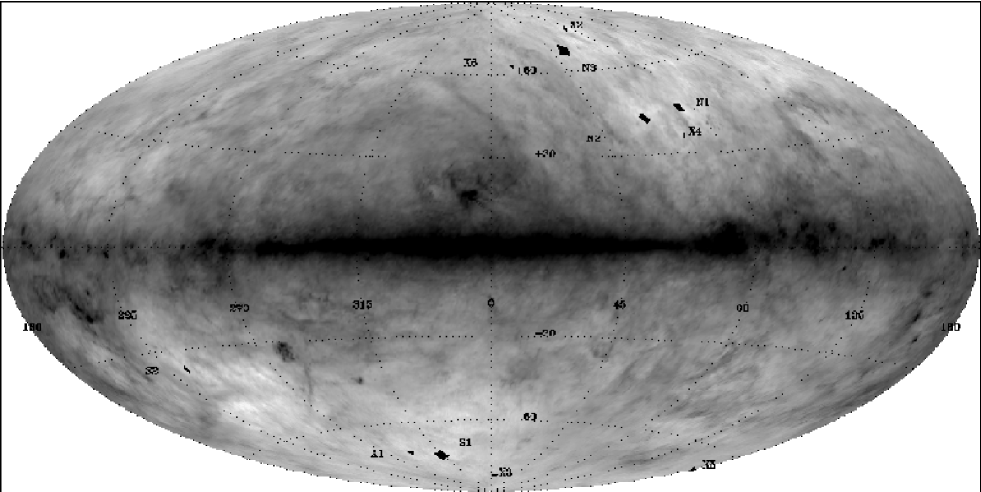
Figure 7: The location of the ELAIS survey fields overlaid on a Hammer-Aitoff equal area projection of the COBE normalised IRAS maps of Schlegel et al. (1998). Galactic latitude and longitude gridlines are overlaid.

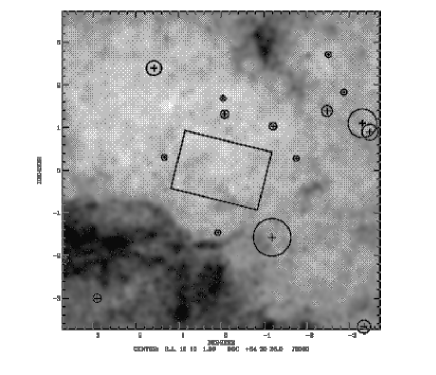
Figure 8: The location of the N1 ELAIS survey field overlaid on the COBE normalised IRAS maps of Schlegel et al. (1998). IRAS sources with 12$\mu$m fluxes brighter than 0.6Jy are overlayed with radius proportional to flux for $S_{60}<10$Jy. The minimum 100$\mu$m intensity shown is 0MJy/sr (white) and the maximum is 1.5MJy/sr (Black).

Figure 9: The location of the N2 ELAIS survey field overlaid on the COBE normalised IRAS maps of Schlegel et al. (1998). IRAS sources with 12$\mu$m fluxes brighter than 0.6Jy are overlayed with radius proportional to flux for $S_{60}<10$Jy. The minimum 100$\mu$m intensity shown is 0MJy/sr (white) and the maximum is 1.5MJy/sr (Black).

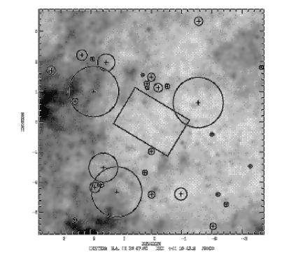
Figure 10: The location of the N3 ELAIS survey field overlaid on the COBE normalised IRAS maps of Schlegel et al. (1998). IRAS sources with 12$\mu$m fluxes brighter than 0.6Jy are overlayed with radius proportional to flux for $S_{60}<10$Jy. The minimum 100$\mu$m intensity shown is 0MJy/sr (white) and the maximum is 1.5MJy/sr (Black).

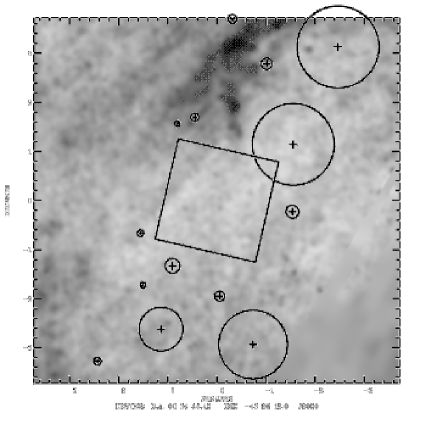
Figure 11: The location of the S1 ELAIS survey field overlaid on the COBE normalised IRAS maps of Schlegel et al. (1998). IRAS sources with 12$\mu$m fluxes brighter than 0.6Jy are overlayed with radius proportional to flux for $S_{60}<10$Jy. The minimum 100$\mu$m intensity shown is 0MJy/sr (white) and the maximum is 1.5MJy/sr (Black).

3.4 Observation Parameters

Table 4 summarises the instrument parameters specified in the majority of our survey AOTs. Most are self explanatory.

For ISO-CAM the $Gain$ was set to 2 which was the standard used for most ISO-CAM observations. $TINT$ was the integration time per readout and $NEXP$ was the number of readouts per pointings (i.e. the total integration time per pointing is $NEXP\times TINT$). $NSTAB$ was the additional number of readouts for the first pointing of a raster added to allow the detector to stabilise.

With ISO-PHOT, $TINT$ was the total integration time per pointing.

The parameters related to the raster geometry ($PFOV$, $NPIX$, $M,N$, $dM,dN$) have the same meaning for each instrument. $PFOV$ is the nominal pixel field of view on the sky. $NPIX$ is the number of pixels along each axis of the detector array. $M,N$ are the number of steps in a raster while $dM,dN$ are the step sizes.

The ISO-CAM rasters were designed such that each sky position was observed twice in successive pointings to improve reliability. To reduce overheads we selected a very large raster size, $40\hbox{${}^{\prime}$}\times 40\hbox{${}^{\prime}$}$. With the exception of small rasters and one test raster, the ISO-CAM parameters remained unchanged throughout the survey.

Since the ISO-PHOT internal calibration measurements were only performed at the beginning and end of a raster we chose these to be half the size of the ISO-CAM rasters ($20\hbox{${}^{\prime}$}\times 40\hbox{${}^{\prime}$}$). We originally used ISO-PHOT with a non-overlapping raster pattern and switched to an overlapping mode during the mission, with most N1 and S1 observations performed in the non-overlapping mode.

The observation parameters for all survey observations are tabulated in Appendix A.

	ISO-CAM		ISO-PHOT
Parameter
Detector	LW	LW	C100	C200
Filter	LW2	LW3	C90	C160
$\lambda/\mu$m	6.75	15	95.1	174
$\Delta\lambda/\mu$m	3.5	6	51.4	89.4
$Gain$	2	2	n/a	n/a
$TINT$/s	2	2	20	32
			12
$NEXP$	10	10	n/a	n/a
$NSTAB$	80	80	n/a	n/a
$PFOV$/′′	6	6	43.5	84.5
$NPIX$	32	32	3	2
$M,N$	28, 14	28, 14	10, 20	13, 13
			20, 20
$dM,dN$/${}^{\prime^{\prime}}$	90, 180	90,180	130, 130	96, 96
			75, 130

Table 4: Summary of the AOT parameters for the bulk of survey programme observations. The 90$\mu$m survey strategy changed after the S1 and N1 observations, and the revised parameters are illustrated. Many observations in N3 and all of the smaller fields X1-6 and S2 were executed with very similar AOTs, but with fewer pointings. Parameters are described in the text and in detail on the ISO WWW pages (http://isowww.estec.esa.nl/).

4 ISO Observations

The ISO observations for the ELAIS programme were executed from 12th March 1996 (revolution 116), 37 days after the beginning of routine operations (4th February 1996, revolution 79) until 17:44 on 8th April 1998 (revolution 875), 10 hours 44 minutes after the first signs of boil off had been detected and 5 hours 23 minutes before the last observations were performed.

In general the execution of the planned observations was very successful. Only three observations were reported as “failed”. Three observations were flagged as “aborted”, all three of these had been concatenated to “failed” observations but appear to have been successfully executed despite this.

The only significant problem in the execution of the survey observations occurred in N3. It transpired that there was a paucity of guide stars in this region and the mission planning team were unable to schedule many of the observations near the original dates requested. To accommodate this problem the sizes of the rasters were reduced and restrictions on the possible observation dates relaxed. However, in the last available observing window for N3 other ISO mission priorities, together with remaining guide star acquisition problems, interfered with the scheduling. The net result is that the coverage of the N3 region is patchy.

It may be that this guide star problems noticed in N3 may be related to an apparent offset of around 6” between the reference frame of the DSS and e.g. the APM catalogue in this field. The APM catalogue agrees very well with the Guide Star Catalogue v1.2 (http://www-gsss.stsci.edu/gsc/gsc12/gsc12_form.html).

4.1 Main Survey Observations

Table 5 indicates the area that has been surveyed at least once in any band in all of our fields. For the four large fields the separation of the raster pointings (40^′) is used to compute the area, i.e. 0.44 square degrees per raster. For the small fields which are not mosaiced the actual size of the raster is used.

The coverage, in terms of integration time per sky pixel, of the four main survey fields (N1-3 and S1) in each of the bands are shown in Figures 12, 13,14,15.

Field	Wavelength/$\mu$m
	6.7	15	90	175
N1		2.67	2.56	2⋆
N2	2.67	2.67	2.67	1
N3	1.32	0.88	1.76
S1	1.76	3.96	3.96
S2	0.12	0.12	0.11	0.11
X1		0.16	0.19
X2		0.16	0.19
X3		0.16	0.19
	5.87	10.78	11.63	3.11
X4		0.09	0.11
X5		0.09
X6		0.09	0.11

Table 5: Survey Fields covered at least once. Areas are given in square degrees.^⋆The 175$\mu$m observations in N1 have been carried out by the FIRBACK team (PI J-L Puget, see Dole et al. [1999]) and are included in this table to illustrate the complete ISO coverage of the ELAIS fields. N1-3, S1-2 and X1-3 are unbiased survey fields, while X4-X6 are centred on known objects so should not be included with the other fields for statistical purposes.

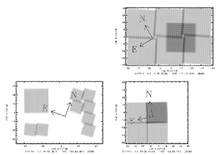
Figure 12: Survey Coverage at 6.7$\mu$mẆhite areas have not been covered at all darker regions indicate longer total integration, either due to repeated observations or overlap, black indicates 200s. The coverage maps have been smoothed to one arc minute resolution. Reading from top left to bottom right the fields are: N2, N3, S1. The true peaks in the coverage are around 150s, 100s and 175s respectively.

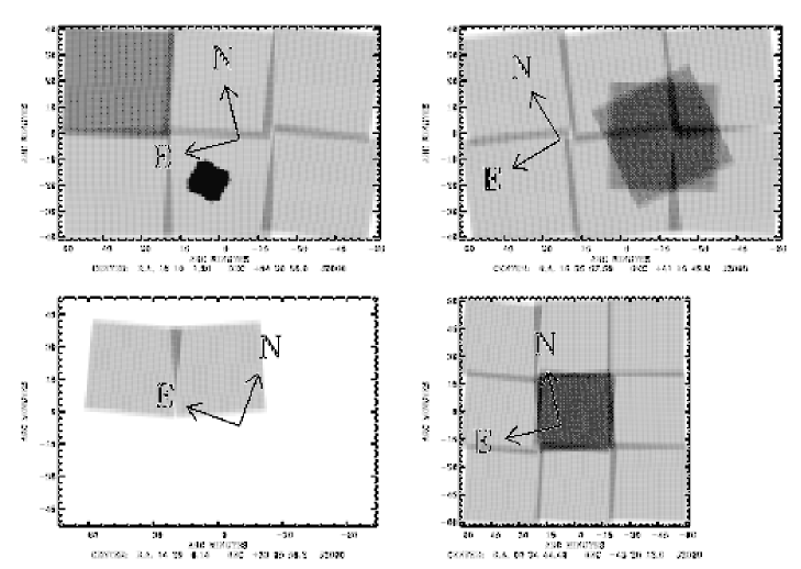
Figure 13: Survey Coverage at 15$\mu$mẆhite areas have not been covered at all darker regions indicate longer total integration, either due to repeated observations or overlap, black indicates 200s. The coverage maps have been smoothed to one arc minute resolution. Reading from top left to bottom right the fields are: N1, N2, N3, S1. The true peaks in the coverage are around 600s, 200s, 100s and 200s respectively.

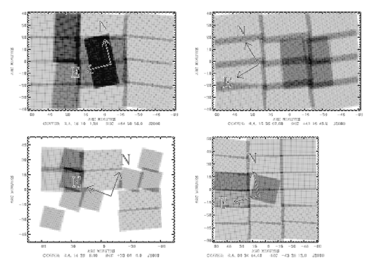
Figure 14: Survey Coverage at 90$\mu$mẆhite areas have not been covered at all darker regions indicate longer total integration, either due to repeated observations or overlap, black indicates 100s. The coverage maps have been smoothed to one arc minute resolution. Reading from top left to bottom right the fields are: N1, N2, N3, S1. The true peaks in the coverage are around 160s, 120s, 120s and 120s respectively.

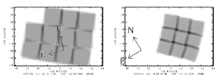
Figure 15: Survey Coverage at 175$\mu$mṄ.B. Only the coverage in N2 is part of the ELAIS project, the coverage in N1 (left) comes from the FIRBACK team (PI J-L. Puget, see Dole et al. [1999]). White areas have not been covered at all darker regions indicate longer total integration, either due to repeated observations or overlap, black indicates 350s. The coverage maps have been smoothed to one arc minute resolution. The true peaks in the coverage are around 260s and 350s respectively.

4.2 Duplicate Survey Observations

A number of sub-fields have been repeated on one or more occasions. This repetition will considerably aid in assessing the reliability and completeness of the survey. In addition this data will provide deeper survey regions which are good targets for more focussed follow-up campaigns and other exploitation.

Table 6 lists all the fields that have repeated observations together with the level of redundancy.

Field	Coordinates (J200)		Wavelength/$\mu$m
			6.7	15	90	175
N1_T	$16^{h}10^{m}01^{s}$	$+54\hbox{${}^{\circ}$}30\hbox{${}^{\prime}$}36\hbox{${}^{\prime\prime}$}$			0.22$\times$3	2$\times$2
					0.22$\times$4
N1_U	$16^{h}11^{m}00^{s}$	$+54\hbox{${}^{\circ}$}13\hbox{${}^{\prime}$}23\hbox{${}^{\prime\prime}$}$		0.04$\times$11
N1_1C	$16^{h}13^{m}54^{s}$	$+54\hbox{${}^{\circ}$}18\hbox{${}^{\prime}$}22\hbox{${}^{\prime\prime}$}$			0.22$\times$2
N_2	$16^{h}13^{m}57^{s}$	$+54\hbox{${}^{\circ}$}59\hbox{${}^{\prime}$}36\hbox{${}^{\prime\prime}$}$	0.44$\times$2
N2	$16^{h}35^{m}45^{s}$	$+41\hbox{${}^{\circ}$}06\hbox{${}^{\prime}$}00\hbox{${}^{\prime\prime}$}$	0.44$\times$2	0.44$\times$3	0.44$\times$3	1$\times$2
N3_5C/D	$14^{h}31^{m}53^{s}$	$+33\hbox{${}^{\circ}$}14\hbox{${}^{\prime}$}37\hbox{${}^{\prime\prime}$}$		0.22$\times$2
S1_5	$00^{h}34^{m}44^{s}$	$-43\hbox{${}^{\circ}$}28\hbox{${}^{\prime}$}12\hbox{${}^{\prime\prime}$}$	0.44$\times$2	0.44$\times$3	0.22$\times$3
S2	$05^{h}02^{m}24^{s}$	$-30\hbox{${}^{\circ}$}35\hbox{${}^{\prime}$}55\hbox{${}^{\prime\prime}$}$		0.12 $\times$4	0.11$\times$5	0.11$\times$3

Table 6: Survey sub-fields covered more than once, listing the area covered (in square degrees) and the number of times that sub-field has been observed.

4.3 Photometry Programme

In addition to the survey observations, we also undertook a photometry programme to observe objects detected early on in the survey programme at other ISO wavelengths.

These objects were selected from the S1 and N1 survey regions which had been observed at an early stage in the campaign. 180 objects which had been detected at 15 $\mu$m were selected to be observed with ISO-CAM at 4.5, 6.7, 9, and 11 $\mu$m using the filters LW-1,LW-2,LW-4 and LW-7. 80 Objects were selected to be observed by ISO-PHOT at 60 and 175 $\mu$m, using the C60, and C160 filters.

The ISO-CAM observations were performed in concatenated chains of 10 pointings. At each pointing a $2\times 1$ raster was performed to ensure accurate photometry and reliable detections. The chains were arranged such that each of the 10 sources was located in a different position on the array (separated by around 18^′′), this was to allow accurate sky flat-fielding over the course of the concatenated chain. The 120 ISO-CAM pointings in S1, and the 80 pointings in N1 were ordered to minimize the total path length, ensuring that sequential observations were as close to each other as possible, both spatially and temporally, improving the flat-fielding.

The ISO-PHOT observations were performed in chains of 15 pointings. On average the 15 pointings contained 5 source positions and 10 background positions. Like the ISO-CAM photometry observations, the ISO-PHOT source positions were ordered to minimize the total path length. The background pointings were chosen to be spaced along this path at reasonably regular intervals, while ensuring that there was at least one background position between every source position.

Other parameters from the AOTs for the photometry programme are summarised in Table 7.

Instrument	ISO-CAM				ISO-PHOT
Parameter
Detector	LW	LW	LW	LW	C100	C200
Filter	LW1	LW2	LW4	LW7	C60	C90
$\lambda/\mu$m	4.5	6.7	6.0	9.62	60.8	174
$\Delta\lambda/\mu$m	1	3.5	1	2.2	23.9	71.7
$Gain$	2	2	2	2	n/a	n/a
$TINT$/s	5	5	5	5	32	32
$NEXP$	8	8	8	8	n/a	n/a
$NSTAB$	50	50	50	50	n/a	n/a
$PFOV/^{\prime\prime}$	6	6	6	6	43.5	84.5
$M,N$	2,1	2,1	2,1	2,1	1,1	1,1
$dM,dN/^{\prime\prime}$	24	24	24	24	n/a	n/1

Table 7: Summary of the AOT parameters for the photometry programme

5 Data Processing and Products

In order to provide targets early on in the campaign to allow follow-up programmes, both from the ground and with ISO, it was decided to perform an initial “Preliminary Analysis”. This was started long before the end of the mission, while the understanding of the behaviour of the instruments was naturally less than it is currently and will be superseded with a “Final Analysis” incorporating the best available knowledge post mission.

The Preliminary Analysis was conducted with the intention of producing reliable source lists at $6.7,15$ and $90\mu$m. The processing of the ISO-CAM survey observations is described in detail by Serjeant et al. [1999] and the reduction of the ISO-PHOT 90$\mu$m survey data will be discussed by Efstathiou et al. (1999, in preparation).

The Final Analysis is currently being undertaken. This is expected to produce better calibrated and fainter source lists than the Preliminary Analysis. The Final Analysis will also produce maps which can be used to determine fluxes or upper-limits for known sources. This analysis will not, however, be completed until early 2000.

The ELAIS products will comprise source catalogues at all wavelengths, 4.5, 6.7, 9, 11, 15, 60, 90, 175, together with maps from all the survey observations. Highly reliable sub-sets of the “Preliminary Analysis” catalogues were released to the community, via our WWW site (http://athena.ph.ic.ac.uk/), concurrent with the expiration of the propriety period on 10th August 1999.

5.1 Data Quality

The quality of the 15 $\mu$m ISO-CAM data is moderately uniform. Some rasters are more affected by cosmic rays than others but the total amount of data seriously affected by cosmic rays is small. The noise levels are within a factor of a few of those expected; a typical noise level is 0.2 ADU/sec/pixel per pointing.

The ISO-PHOT data is seriously affected by cosmic rays and detector drifts. We have used the fluctuations in the time sequence of each pixel as an estimate of the average noise level. The fluctuations per pointing were typically 3 per cent of the background level, though 3 of the 9 pixels were noisier with fluctuations typically 4 per cent of the background. A few observations showed higher noise due to increased cosmic ray hits. Our original AOTs employed an integration time of 20s. We subsequently decreased this to 12s to allow for an overlapping raster giving a factor of two redundancy with similar observation time. Importantly there does not appear to be a significant difference in noise levels per pointing despite the factor of two reduction in integration time, indicating that non-white noise in the pixel histories is dominant. The redundancy introduced by this new strategy could improve the signal to noise ratio for sources by as much as $\sqrt{2}$.

5.2 Preliminary Data Analysis

The processing for the ISO-PHOT and ISO-CAM data proceeds in a similar fashion. All data reduction used a combination of standard routines from the PHOT Interactive Analysis [1996] ) software and the CAM Interactive Analysis [1998] together with purpose-built IDL routines. The frequency of glitches and other transient phenomena led to non-Gaussian and non-white-noise behaviour.

A number of data reduction techniques were tested at ICSTM, CEA/SACLAY, IAS and MPIA. Parallel pipeline processes for reducing the ISO-PHOT data were run at both ICSTM and MPIA. Data reduction techniques suitable for ISO-CAM data with multiple redundancy, such as the observations of the Hubble Deep Field [1997], e.g. the Pattern REcognition Technique for ISO-CAM data [1999] were unsuccessful in processing this data. The most reliable approach for source extraction was found to be looking for source profiles in the time histories of individual pixels rather than by constructing sky maps.

For both instruments the data stream from each detector pixel was treated as an independent scan of the sky. These data streams were filtered to remove glitches and transients and averaged to produce a single measurement at each pointing position. Significant outliers remaining in the data streams were flagged as potential sources. For the ISO-CAM observations the redundancy of the pointings was used to provide confirmation of candidate sources. The data stream surrounding all remaining candidates was then examined independently by at least two observers to remove spurious detections. Sources that were acceptable to two or more observers were classified as good ($REL=2$) and those acceptable to only one observer were classified as marginal $(REL=3)$.

The fraction of spurious detections was high due to the non-Gaussian nature of the noise and relatively low thresholds applied. More than 13 thousand ISO-PHOT source candidates were examined as were just over 15 thousand ISO-CAM 15 $\mu$m candidates. At 6.7 $\mu$m the rejected fraction was lower and the candidate list was only 3 thousand. The final numbers of objects in the Preliminary Catalogue Version 1.3 are tabulated in Table 8

	Wavelength
Quality	6.7$\mu$m	15 $\mu$	90$\mu$
Good $(REL=2)$	795	728	153
Moderate $(REL=3)$	2341	818	208

Table 8: ELAIS Preliminary Source Catalogue Statistics

The “eye-balling” technique while laborious ensured that the resulting catalogues are highly reliable, as discussed in greater detail in Serjeant et al. [1999] and Efstathiou et al. (1999., in preparation). The sub-sets of the Preliminary Catalogues that were released to the community were those ISO-PHOT sources that had been confirmed by four observers, and those ISO-CAM sources that had been confirmed by two observers with fluxes above 4mJy, these sub-sets are exceptionally reliable.

A “Final Analysis” process has been developed which uses the transient correction techniques of Lari (1999, in preparation). These techniques have been shown to be excellent for reducing ISO-CAM data. While this is almost certainly the best procedure for reducing the ELAIS data, it is labour intensive and time consuming and we do not expect the “Final Analysis” to be finished until early 2000, hence the release of our “Preliminary” products.

5.3 Source Calibration

For the ISO-CAM observations we have of order 10 stars per raster and these provide a very good calibration. A preliminary analysis of the star fluxes (Crockett et al. 1999 in preparation, see also Serjeant et al. 1999) suggests that our raw instrumental units (ADU/g/s) need to be multiplied by a factor of 1.75 to give fluxes in mJy. This implies a $50$ per cent completeness limit of approximately $3$ mJy at $15\mu$m. The flux calibration is still uncertain at $6.7\mu$m, due largely to the uncertain aperture corrections to the under-sampled observations and the single-pixel detection algorithm, though PSF models and pre-flight sensitivity estimates suggest a $50$ per cent completeness level at less than $1$mJy. (See Serjeant et al. [1999] for more details.)

For the 90 $\mu$m survey the calibration proceeded as follows. The expected background was estimated using COBE and IRAS data and Zodiacal light models. These predictions were compared to the measurements of the background calibrated using the internal calibration device (FCS) allowing the predicted backgrounds to be corrected from an extended source to a point source calibration. These predictions were then used to scale the measured fluctuations above the background. Single pixel detections (“Point sources”) were then calibrated using the expected fraction of flux falling on a single pixel for a source placed arbitrarily with respect to the pixel centre. The fluxes of “extended sources” were calculated in a more complicated fashion and have great associated uncertainties. The fluxes were found to be in good agreement with model stellar fluxes in our own dedicated calibration measurements and with the fluxes of IRAS sources in the fields. This suggests a 5$\sigma$ noise level of 100mJy. This ISO-PHOT calibration, completeness and reliability estimates is discussed in detail by Efstathiou et al. (1999, in preparation) and Surace et al. (1999, in preparation).

6 Comparison with Other ISO Surveys

ISO carried out a variety of complementary surveys exploring the available parameter space of depth and area. Table 9 summaries the main extra-galactic blank-field surveys. With the exception of the two main serendipity surveys ELAIS covers the largest area and has produced the largest number of ISO sources. Figure 16 illustrates how deeper smaller area surveys are complemented by shallower wider area surveys.

Survey Name	[e.g. ref]	Wavelength	Integration	Area
		$/\mu$m	$/$s	$/{\rm sqdeg}$
PHT Serendipity Survey	1	175	0.5	7000
CAM Parallel Mode	2	6.7	150	33
ELAIS	3	6.7,15,90,175	40, 40, 24, 128	6, 11, 12,1
CAM Shallow	4	15	180	1.3
FIRBACK	5	175	256, 128	1, 3
IR Back	6	90, 135,180	23, 27, 27	1, 1, 1
SA 57	6.7	60, 90	150, 50	0.42,0.42
CAM Deep	8	6.7, 15, 90	800, 990, 144	0.28, 0.28, 0.28
Comet fields	9	12	302	0.11
CFRS	10	6.7,15,60,90	720, 1000, 3000,3000	0.067.0.067.0.067,0.067
CAM Ultra-Deep	11	6.7	3520	0.013
ISOHDF South	12	6.7, 15	$>6400,>6400$	4.7e-3, 4.7e-3
Deep SSA13	13	6.7	34000	2.5e-3
Deep Lockman	14,15	6.7, 90, 175	44640, 48, 128	2.5e-3, 1.2 , 1
ISOHDF North	15	6.7, 15	12800, 6400	1.4e-3, 4.2e-3

Table 9: Field Surveys with ISO, ordered roughly in decreasing area. References: 1 – Bogun et al. [], 2 – Siebenmorgen et al. [1996], 3 – this paper, 4 – Elbaz et al. [1999], 5 – Dole et al. [1999], 6 – Mattila et al. (1999, in prep.), 7 – Linden-Vørnle[1997], 8 – Elbaz et al. [1999] 9 – Clements et al. [1999], 10 – Flores et al. [1999a],[1999b], 11 – Elbaz et al. [1999], 12 – Oliver et al. (1999, in preparation), 13 – Taniguchi et al. [1997a], 14 – Taniguchi et al. [1997b], 15 – Kawara et al. [1998], 16 – Serjeant et al. [1997]

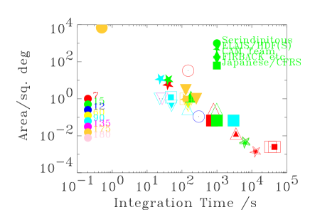
Figure 16: Figure comparing ISO surveys area vs. depth. All the surveys in Table 9 are plotted. The ELAIS points have an additional outline.

7 Follow-up

An extensive follow-up programme is being undertaken, including observations in many bands from X-ray to radio. This programme will provide essential information for identifying the types of objects detected in the infrared, their luminosities, energy budgets and other detailed properties. As well as studying the properties of the objects detected by ISO a number of the follow-up surveys will provide independent source lists which will be extremely valuable in their own right, e.g. to investigate the differences between infrared and non infrared emitting objects.

7.1 Surveys

A number of follow-up programmes are in fact independent surveys at other wavelengths, carried out within the ELAIS survey area. These include:

1. Optical: $R$-band CCD surveys are essential to provide optical identifications for spectroscopic and related follow-up with improved astrometry, photometric accuracy and to fainter levels than those provided by the Second Sky Survey. Our principal southern field (S1) has been completely covered with the ESO/Danish 1.5m telescope to a depth of $R\sim 23.5$ (La Franca et al. 1999, in preparation), while all our northern fields N1-3 have been completed to a similar depth using the INT Wide Field Camera (Verma et al. 1999, in preparation). Other optical bands allow object classification and other more detailed investigations. Four square degrees within our northern fields have been observed to a depth of $U\sim 22$ (Verma et al. 1999, in preparation). In June 1999, we observed the central 1.2 square degrees of S1 in $U$ and 3 square degrees in $I$ using the ESO Wide Field Imager (Héraudeau et al. 1999, in preparation) with these we expect to reach $U\sim 23,I\sim 23$. McMahon et al. (http://www.ast.cam.ac.uk/~rgm/int_sur/) have covered around 9 square degrees of N1 to $u\sim 23.3,g\sim 24.2,r\sim 23.5,i\sim 22.7,z\sim 21.1$ and 2 square degrees in N2 to similar depths in $g,r,i,z$ as part of the ING wide field survey. The $U$-band surveys will be especially interesting as they will allow us to compute the $U$-band luminosity density (and hence star formation rate) in the same volume as we calculate the infrared luminosity density, providing a direct comparison between obscured and unobscured star formation estimators.

2. Near Infrared: A substantial area has been surveyed in the near infrared. In the $H$-band around 0.85 square degrees in N1 and N2 was surveyed using CIRSI on the INT (Gonzalez-Solares et al. 1999, in preparation). Approximately 0.5 square degree has been surveyed in both N1 and N2 in $K^{\prime}$ using Omega Prime on the Calar Alto 3.5m (Rigopoulou et al. 1999, in preparation). The smaller, multiply repeated southern field S2 has been covered in $K$ with SOFI on the NTT (Héraudeau et al., 1999, in preparation).

3. Radio: 21cm radio data at sub-mJy level will allow identification of some of the most interesting objects which are expected to be very faint in the optical but would have detectable radio fluxes if they obey the usual radio to far infrared correlation. These surveys will also allow an independent estimate of the star formation rate within the same volume. The southern field S1 is completely covered to a depth of 0.3 mJy [1999], the 6 square degrees in the northern fields has been covered to a depth of 0.2 mJy [1999]. A deeper survey in the south has been conducted on the smaller, multiply repeated field S2 (Gruppioni et al. 1999, in preparation).

4. X-ray: Almaini et al. have been awarded 150ks to do two deep Chandra pointings one in N1 and one in N2. La Franca et al. have also been awarded 200 ks on BeppoSAX to make 5 pointings covering around 2 square degrees in S1.

5. Sub-mm: The UK SCUBA Survey consortium (Rowan-Robinson et al., independent of ELAIS) are performing part of their shallow (8mJy) 850$\mu$msurvey in N1 and N2 and are aiming to cover 200 square arc minutes in each.

Band	2-10keV	$u,g,r,i,z$	$R$	$H$	$K$	6.7	15	90	175	850	21cm
Depth Units	CGI	mag	mag	mag	mag	mJy	mJy	mJy	mJy	mJy	mJy
N1
Area	0.07	9	3.1	0.5	0.4		2.6	2.6	2	0.05	1.54
Depth	$10^{-14}$	23.3,24.2,23.5,22.7,21.1	23	19.5	18.0	1	3	100	100	8	0.1-0.4
N2
Area	0.07	2	3.6	0.5	0.4	2.7	2.7	2.7	1	0.05	1.54
Depth	$10^{-14}$	22.5,24.2,23.5,22.7,21.1	23	19.5	18.0	1	3	100	100	8	0.1-0.4
N3
Area		1,1,2.3,1,0	2.3	1		1.32	0.9	1.76			1.14
Depth		22.5,23,23,23,0	23	19.5		1	3	100			0.1-0.4
S1
Area	2	1.2,0,4,3,0	4			1.8	4	4			4
Depth	$10^{-13}$	23,0,23.5,23,0	23.5			1	3	100			0.24

Table 10: Multi-wavelength field surveys within the main ELAIS fields, the vast majority carried out as part of the ELAIS collaboration. Areas are in square degrees. Some sub-fields within these go to greater depth. The X-ray and sub-mm surveys are yet to be completed.

Additional multi-wavelength surveys of these fields are expected in the near future.

7.2 Photometry & Spectroscopy

We intend to obtain spectroscopic identifications for all (or the vast majority) of optical candidates for all ELAIS sources. This involves a two-pronged attack using multi-object spectroscopy for the brightest objects and single object spectroscopy using 4m class telescopes on the fainter objects. This will be principally to obtain the redshifts and thus luminosity but also for classification and to assess star formation rates. Some preliminary multi-fibre spectroscopy has been carried out with FLAIR on the UK Schmidt Telescope. This been supplemented by single object spectroscopy from the ESO/Danish 1.5m telescope to provide spectroscopy on a complete sample of 90$\mu$m selected sources (Linden-Vørnle et al. 1999, in preparation). A further 100 sources have been identified spectroscopically in a largely weathered-out run on the 2dF in September 1998 (Gruppioni et al. 1999, in preparation) and an additional night on the 2dF in August 1999 was also seriously hampered by weather (Oliver et al. 1999, in preparation). 40 spectra for fainter sources have already been taken with EMMI on the NTT and EFOSC2 on the ESO 3.6m Telescope (La Franca et al. 1999, in preparation).

Until now the ELAIS northern fields have been only moderately surveyed spectroscopically. We have used the Calar Alto 2.2m telescope and the Calar Alto Faint Object Spectrograph (CAFOS) for the sources brighter than 17 (Gonzalez-Solares et al. 1999, in preparation) and the Calar Alto 3.5m telescope and the Multi Object Spectrograph (MOSCA) for the fainter sources (Surace et al., 1999, in preparation). 29 ELAIS objects have been observed during the period May-July 1998 (of which 14 had $m>19$). These observations have been completed with 29 field galaxies chosen in the same region for comparison purpose. From these northern samples most sources show strong star-burst signatures up to $z=0.5$ though two AGNs and one $z=1.2$ QSO have been detected, these samples will be discussed in a forthcoming paper.

A number of programmes have been instigated to obtain more specific photometric and spectroscopic data of the infrared selected sources over a wider wavelength range. Some examples are detailed below:

1. We have observed (Héraudeau, Kotilainen, Surace et al., in preparation) about 150 sources in pointing observations in the S1 field using IRAC2 on the ESO/MPG 2.2m telescope October 1997, June 1998 and SOFI on the NTT October 1998

2. Near-infrared H+K band spectroscopy of a small subset of sources with SOFI on the NTT (Alexander et al., in preparation).

8 Conclusions

In this paper we have described the motivation behind ELAIS, the largest non-serendipitous survey performed by ISO. Our primary goals in conducting the survey were to determine the relative importance and recent evolution of the dust–obscured mode of star formation in galaxies, and to constrain AGN unification models, and we detailed above how these influenced our selection of survey fields and observational parameters. The fields that have been covered by ISO are also being extensively mapped from radio to X–ray wavelengths as part of a concerted ground–based follow–up programme, whose multi–wavelength coverage will make the ELAIS regions fertile ground for undertaking future astrophysical investigations extending well beyond our initial survey aims.

Subsequent papers in this series will discuss in detail the scientific results from the ELAIS “Preliminary Analysis” and “Final Analysis”. The first of these papers will include: discussions of the extra-galactic counts from the “Preliminary Analysis” at 7 and 15 $\mu$m(Serjeant et al. 1999), and at 90$\mu$m (Efstathiou et al., 1999, in preparation); discussion of the stellar calibration and counts (Crockett et al., in preparation); and a discussion of sources detected in the multiply–repeated areas (Oliver et al., in preparation). Preliminary ELAIS data products were released through our WWW page (http://athena.ph.ic.ac.uk/), which also contains further details on the programme and the follow-up campaign.

Appendix A Log of the ISO Observations

In Table A1 we present a list of all the observations performed by ISO as part of the ELAIS raster observations. We do not include the observations performed as part of the ISO photometric follow-up of ELAIS sources which are available on our WWW pages http://athena.ph.ic.ac.uk/. Table 14 details those observations which have had some instrument or telemetry problems as flagged at Vilspa or for which we have noted peculiarities.

Table 11: Log of all the ISO survey observations performed for ELAIS, excluding the pointed photometric observations. TDN is a unique identifier for each ISO observation and monotonically increased throughout the mission. OFFICIAL$\_$NAME is a unique identifier for ELAIS observations constructed from the instrument name, the filter, the main field identifier and where required a sub-field identifier and a multiplicity identifier, it does not correspond to the name in the ISO archives.

TDN	OFFICIAL$\_$NAME	RA (J2000) Dec(J2000)	ROLL	M	N	DM	DN	TINT	FILT	STATUS
11600721	CAM$\_$LW3$\_$N2$\_$T$\_$I	16 35 45.00 +41 06 00.0	84	28	14	90	180	21	LW3	Observed
19201010	PHT$\_$C90$\_$N1$\_$T$\_$I	16 10 01.20 +54 30 36.0	358	10	20	130	130	10	90	Observed
19201091	PHT$\_$C90$\_$N1$\_$T$\_$J	16 10 01.20 +54 30 36.0	358	10	20	130	130	32	90	Observed
23200251	CAM$\_$LW3$\_$S1$\_$1	00 30 25.40 -42 57 00.3	77	28	14	90	180	21	LW3	Observed
23200252	PHT$\_$C90$\_$S1$\_$1A	00 30 14.90 -42 47 11.7	78	10	20	130	130	20	90	Observed
23200289	PHT$\_$C90$\_$S1$\_$1B	00 30 36.00 -43 06 48.8	78	10	20	130	130	20	90	Observed
23200353	CAM$\_$LW3$\_$S1$\_$2	00 31 08.20 -43 36 14.1	78	28	14	90	180	21	LW3	Observed
23200354	PHT$\_$C90$\_$S1$\_$2A	00 30 57.40 -43 26 25.7	78	10	20	130	130	20	90	Observed
23200392	PHT$\_$C90$\_$S1$\_$2B	00 31 19.00 -43 46 02.5	78	10	20	130	130	20	90	Observed
23300257	CAM$\_$LW3$\_$S1$\_$4	00 33 59.40 -42 49 03.1	77	28	14	90	180	21	LW3	Observed
23300258	PHT$\_$C90$\_$S1$\_$4A	00 33 48.30 -42 39 15.8	77	10	20	130	130	20	90	Observed
23300294	PHT$\_$C90$\_$S1$\_$4B	00 34 10.60 -42 58 50.4	78	10	20	130	130	20	90	Observed
23300459	CAM$\_$LW3$\_$S1$\_$5	00 34 44.40 -43 28 12.0	78	28	14	90	180	21	LW3	Observed
23300460	PHT$\_$C90$\_$S1$\_$5A	00 34 33.10 -43 18 24.9	78	10	20	130	130	20	90	Observed
23300495	PHT$\_$C90$\_$S1$\_$5B	00 34 55.80 -43 37 59.1	78	10	20	130	130	20	90	Observed
30200101	CAM$\_$LW3$\_$N1$\_$1	16 15 01.00 +54 20 41.0	258	28	14	90	180	21	LW3	Observed
30200102	PHT$\_$C90$\_$N1$\_$1A	16 15 16.70 +54 10 57.0	258	10	20	130	130	20	90	Observed
30200113	PHT$\_$C90$\_$N1$\_$1B	16 14 45.30 +54 30 24.9	258	10	20	130	130	20	90	Observed
30400103	CAM$\_$LW3$\_$N1$\_$2	16 13 57.10 +54 59 35.9	255	28	14	90	180	21	LW3	Aborted
30400104	PHT$\_$C90$\_$N1$\_$2A	16 14 13.30 +54 49 52.4	256	10	20	130	130	20	90	Failed
30400114	PHT$\_$C90$\_$N1$\_$2B	16 13 40.90 +55 09 19.3	255	10	20	130	130	20	90	Aborted
30500105	CAM$\_$LW3$\_$N1$\_$3	16 10 34.90 +54 11 12.7	254	28	14	90	180	21	LW3	Observed
30500106	PHT$\_$C90$\_$N1$\_$3A	16 10 51.50 +54 01 30.9	254	10	20	130	130	20	90	Observed
30500115	PHT$\_$C90$\_$N1$\_$3B	16 10 18.10 +54 20 54.4	254	10	20	130	130	20	90	Observed
30600107	CAM$\_$LW3$\_$N1$\_$4	16 09 27.00 +54 49 58.7	253	28	14	90	180	21	LW3	Observed
30600108	PHT$\_$C90$\_$N1$\_$4A	16 09 44.20 +54 40 17.4	253	10	20	130	130	20	90	Observed
30600116	PHT$\_$C90$\_$N1$\_$4B	16 09 09.70 +54 59 39.8	252	10	20	130	130	20	90	Observed
30900111	CAM$\_$LW3$\_$N1$\_$6	16 04 59.00 +54 39 44.3	249	28	14	90	180	21	LW3	Observed
30900112	PHT$\_$C90$\_$N1$\_$6A	16 05 17.20 +54 30 05.5	249	10	20	130	130	20	90	Observed
30900118	PHT$\_$C90$\_$N1$\_$6B	16 04 40.70 +54 49 22.9	249	10	20	130	130	20	90	Observed
31000109	CAM$\_$LW3$\_$N1$\_$5	16 06 10.80 +54 01 08.0	248	28	14	90	180	21	LW3	Observed
31000117	PHT$\_$C90$\_$N1$\_$5B	16 05 53.10 +54 10 47.3	248	10	20	130	130	20	90	Observed
31000132	PHT$\_$C90$\_$N1$\_$5A	16 06 28.40 +53 51 28.6	248	10	20	130	130	20	90	Observed
40700479	CAM$\_$LW3$\_$X6$\_$1	14 36 43.10 +15 44 13.0	124	12	6	90	180	21	LW3	Observed
40700480	PHT$\_$C90$\_$X6$\_$1	14 36 43.10 +15 44 13.0	124	9	9	130	130	20	90	Observed
40701983	CAM$\_$LW3$\_$X4$\_$1	17 14 14.00 +50 15 23.6	163	12	6	90	180	21	LW3	Observed
40701984	PHT$\_$C90$\_$X4$\_$1	17 14 14.00 +50 15 23.6	162	9	9	130	130	20	90	Observed
40800464	PHT$\_$C90$\_$S1$\_$7A	00 37 20.80 -42 30 55.3	251	10	20	130	130	20	90	Observed
40800497	PHT$\_$C90$\_$S1$\_$7B	00 37 44.20 -42 50 27.1	251	10	20	130	130	20	90	Observed
40800663	CAM$\_$LW3$\_$S1$\_$7	00 37 32.50 -42 40 41.2	251	28	14	90	180	21	LW3	Observed
40800765	CAM$\_$LW3$\_$S1$\_$8	00 38 19.60 -43 19 44.5	251	28	14	90	180	21	LW3	Observed
41000856	PHT$\_$C90$\_$S1$\_$3A	00 31 40.90 -44 05 38.9	254	10	20	130	130	20	90	Observed
41000893	PHT$\_$C90$\_$S1$\_$3B	00 32 03.00 -44 25 15.0	254	10	20	130	130	20	90	Observed
41001062	PHT$\_$C90$\_$S1$\_$6A	00 35 18.80 -43 57 33.0	253	10	20	130	130	20	90	Observed
41001096	PHT$\_$C90$\_$S1$\_$6B	00 35 42.00 -44 17 06.4	253	10	20	130	130	20	90	Observed
41001161	CAM$\_$LW3$\_$S1$\_$6	00 35 30.40 -44 07 19.8	253	28	14	90	180	21	LW3	Observed
41101867	CAM$\_$LW3$\_$S1$\_$9	00 39 07.80 -43 58 46.6	253	28	14	90	180	21	LW3	Observed
41300766	PHT$\_$C90$\_$S1$\_$8A	00 38 07.70 -43 09 58.8	255	10	20	130	130	20	90	Failed
41300798	PHT$\_$C90$\_$S1$\_$8B	00 38 31.60 -43 29 30.2	255	10	20	130	130	32	90	Aborted
41300955	CAM$\_$LW3$\_$S1$\_$3	00 31 51.90 -44 15 27.0	256	28	14	90	180	21	LW3	Observed
41301068	PHT$\_$C90$\_$S1$\_$9A	00 38 55.70 -43 49 01.2	255	10	20	130	130	20	90	Observed
41301099	PHT$\_$C90$\_$S1$\_$9B	00 39 20.00 -44 08 31.8	255	10	20	130	130	20	90	Observed
41502787	CAM$\_$LW3$\_$X3$\_$1	00 22 48.00 -30 06 30.0	254	16	16	90	90	21	LW3	Observed
41502788	PHT$\_$C90$\_$X3$\_$1	00 22 48.00 -30 06 30.0	254	12	12	130	130	20	90	Observed
42500136	PHT$\_$C90$\_$N3$\_$2A	14 25 49.90 +33 09 53.8	114	10	20	130	130	20	90	Observed
42500146	PHT$\_$C90$\_$N3$\_$2B	14 25 18.60 +32 51 00.7	114	10	20	130	130	20	90	Observed
42500237	CAM$\_$LW3$\_$N3$\_$3	14 29 38.30 +33 24 49.6	114	28	14	90	180	21	LW3	Observed
42700238	PHT$\_$C90$\_$N3$\_$3A	14 29 54.50 +33 34 14.2	113	10	20	130	130	20	90	Observed
42700247	PHT$\_$C90$\_$N3$\_$3B	14 29 22.10 +33 15 24.9	113	10	20	130	130	20	90	Observed
43800341	CAM$\_$LW3$\_$N3$\_$5	14 32 38.20 +33 11 10.3	105	28	14	90	180	21	LW3	Observed

Table 12: continued

Log of all the ISO survey observations performed for ELAIS, excluding the pointed photometric observations. TDN OFFICIAL$\_$NAME RA (J2000) Dec(J2000) ROLL M N DM DN TINT FILT STATUS 49900120 PHT$\_$C90$\_$N2$\_$1A 16 32 33.00 +41 22 14.3 247 20 20 75 130 12 90 Observed 49900222 PHT$\_$C90$\_$N2$\_$1B 16 33 26.50 +41 04 51.7 247 20 20 75 130 12 90 Observed 49900326 PHT$\_$C90$\_$N2$\_$2B 16 35 10.50 +40 30 02.0 248 20 20 75 130 12 90 Observed 50000124 PHT$\_$C90$\_$N2$\_$2A 16 34 18.30 +40 47 27.6 247 20 20 75 130 12 90 Observed 50000228 PHT$\_$C90$\_$N2$\_$3A 16 35 39.40 +41 41 55.6 247 20 20 75 130 12 90 Observed 50000330 PHT$\_$C90$\_$N2$\_$3B 16 36 31.30 +41 24 27.7 247 20 20 75 130 12 90 Observed 50000723 CAM$\_$LW3$\_$N2$\_$3 16 36 05.50 +41 33 11.8 247 28 14 90 180 21 LW3 Observed 50100172 PHT$\_$C90$\_$N2$\_$4B 16 38 14.20 +40 49 27.6 246 20 20 75 130 12 90 Observed 50100273 PHT$\_$C90$\_$N2$\_$5A 16 38 47.80 +42 01 18.0 246 20 20 75 130 12 90 Observed 50100374 PHT$\_$C90$\_$N2$\_$5B 16 39 39.70 +41 43 44.9 246 20 20 75 130 12 90 Observed 50100727 CAM$\_$LW3$\_$N2$\_$5 16 39 13.80 +41 52 31.6 246 28 14 90 180 21 LW3 Observed 50100871 PHT$\_$C90$\_$N2$\_$4A 16 37 23.50 +41 06 58.3 246 20 20 75 130 12 90 Observed 50200119 CAM$\_$LW3$\_$N2$\_$1 16 32 59.80 +41 13 33.2 244 28 14 90 180 21 LW3 Observed 50200225 CAM$\_$LW3$\_$N2$\_$4 16 37 48.90 +40 58 13.1 245 28 14 90 180 21 LW3 Observed 50200429 CAM$\_$LW3$\_$N2$\_$6 16 40 55.50 +41 17 22.7 246 28 14 90 180 21 LW3 Observed 50200575 PHT$\_$C90$\_$N2$\_$6A 16 40 30.10 +41 26 10.4 246 20 20 75 130 12 90 Observed 51100131 CAM$\_$LW3$\_$N2$\_$2 16 34 44.50 +40 38 45.0 236 28 14 90 180 21 LW3 Observed 51100234 CAM$\_$LW2$\_$N2$\_$4 16 37 48.90 +40 58 13.1 236 28 14 90 180 21 LW2 Observed 51100736 CAM$\_$LW2$\_$N2$\_$6 16 40 55.50 +41 17 22.7 237 28 14 90 180 21 LW2 Observed 51100835 CAM$\_$LW2$\_$N2$\_$5 16 39 13.80 +41 52 31.6 236 28 14 90 180 21 LW2 Observed 51200131 CAM$\_$LW2$\_$N2$\_$1 16 32 59.80 +41 13 33.2 234 28 14 90 180 21 LW2 Observed 51200232 CAM$\_$LW2$\_$N2$\_$2 16 34 44.50 +40 38 45.0 235 28 14 90 180 21 LW2 Observed 51200433 CAM$\_$LW2$\_$N2$\_$3 16 36 05.50 +41 33 11.8 235 28 14 90 180 21 LW2 Observed 51200576 PHT$\_$C90$\_$N2$\_$6B 16 41 20.80 +41 08 34.6 236 20 20 75 130 12 90 Observed 54502485 CAM$\_$LW3$\_$X1$\_$1 01 13 12.80 -45 14 06.7 33 16 8 90 180 21 LW3 Observed 54502486 PHT$\_$C90$\_$X1$\_$1 01 13 12.80 -45 14 06.7 33 12 12 130 130 20 90 Observed 59800143 CAM$\_$LW2$\_$S1$\_$5 00 34 44.40 -43 28 12.0 76 28 14 90 180 21 LW2 Observed 59800244 CAM$\_$LW2$\_$S1$\_$6 00 35 30.40 -44 07 19.8 77 28 14 90 180 21 LW2 Observed 59800745 CAM$\_$LW2$\_$S1$\_$8 00 38 19.60 -43 19 44.5 77 28 14 90 180 21 LW2 Observed 59800846 CAM$\_$LW2$\_$S1$\_$9 00 39 07.80 -43 58 46.6 77 28 14 90 180 21 LW2 Observed 61300341 CAM$\_$LW2$\_$N3$\_$5 14 32 38.20 +33 11 10.3 291 28 14 90 180 21 LW2 Observed 61600642 PHT$\_$C90$\_$N3$\_$5A 14 32 54.70 +33 20 33.4 289 20 20 75 130 12 90 Observed 61600649 PHT$\_$C90$\_$N3$\_$5B 14 32 21.70 +33 01 47.0 289 20 20 75 130 12 90 Observed 61800277 CAM$\_$LW3$\_$X2$\_$1 13 34 36.00 +37 54 36.0 280 16 8 90 180 21 LW3 Observed 61800278 PHT$\_$C90$\_$X2$\_$1 13 34 36.00 +37 54 36.0 279 12 12 130 130 20 90 Observed 62300324 CAM$\_$LW2$\_$N3$\_$6D 14 32 01.00 +32 20 47.0 285 14 7 90 180 21 LW2 Observed 62300422 CAM$\_$LW2$\_$N3$\_$6B 14 30 32.00 +32 27 37.0 284 14 7 90 180 21 LW2 Observed 63500448 PHT$\_$C90$\_$N3$\_$6D 14 32 01.00 +32 20 47.0 277 10 20 130 65 12 90 Observed 63500539 PHT$\_$C90$\_$N3$\_$4C 14 29 34.80 +32 53 13.0 276 10 20 130 65 12 90 Observed 63500628 PHT$\_$C90$\_$N3$\_$1D 14 27 06.80 +33 25 28.0 275 10 20 130 65 12 90 Observed 63500726 PHT$\_$C90$\_$N3$\_$1B 14 25 36.30 +33 32 04.0 275 10 20 130 65 12 90 Observed 63500825 PHT$\_$C90$\_$N3$\_$1A 14 26 07.90 +33 50 57.0 275 10 20 130 65 12 90 Observed 63501041 PHT$\_$C90$\_$N3$\_$5C$\_$I 14 32 09.70 +33 24 00.0 276 10 20 130 65 12 90 Observed 63501142 PHT$\_$C90$\_$N3$\_$5D$\_$I 14 31 36.90 +33 05 13.0 276 10 20 130 65 12 90 Observed 63800106 CAM$\_$LW2$\_$N3$\_$2B 14 24 33.60 +32 54 17.0 273 14 7 90 180 21 LW2 Observed 63800205 CAM$\_$LW2$\_$N3$\_$2A 14 25 04.80 +33 13 11.0 273 14 7 90 180 21 LW2 Observed 63800302 CAM$\_$LW2$\_$N3$\_$1B 14 25 36.30 +33 32 04.0 273 14 7 90 180 21 LW2 Observed 63800401 CAM$\_$LW2$\_$N3$\_$1A 14 26 07.90 +33 50 57.0 273 14 7 90 180 21 LW2 Observed 63800504 CAM$\_$LW2$\_$N3$\_$1D 14 27 06.80 +33 25 28.0 272 14 7 90 180 21 LW2 Observed 63800603 CAM$\_$LW2$\_$N3$\_$1C 14 27 38.70 +33 44 19.0 272 14 7 90 180 21 LW2 Observed 63800745 PHT$\_$C90$\_$N3$\_$6A 14 31 04.40 +32 46 25.0 273 10 20 130 65 12 90 Failed 67200103 CAM$\_$LW3$\_$N1$\_$2$\_$I 16 13 57.10 +54 59 35.9 254 28 14 90 180 21 LW3 Observed 67200114 PHT$\_$C90$\_$N1$\_$2C 16 12 49.40 +54 57 15.1 254 20 20 130 65 20 90 Observed 67500104 PHT$\_$C90$\_$N1$\_$1C$\_$I 16 13 54.30 +54 18 22.3 251 20 20 130 65 12 90 Observed 75200310 PHT$\_$C90$\_$N1$\_$T$\_$K 16 11 09.60 +54 31 52.7 171 10 20 130 130 12 90 Observed 75200411 PHT$\_$C90$\_$N1$\_$T$\_$L 16 08 52.90 +54 29 16.9 170 10 20 130 130 12 90 Observed 75200512 PHT$\_$C90$\_$N1$\_$T$\_$M 16 09 52.10 +54 40 30.9 170 20 10 130 130 12 90 Observed 75200613 PHT$\_$C90$\_$N1$\_$T$\_$F 16 10 10.10 +54 20 41.1 171 20 10 130 130 12 90 Observed 75901219 PHT$\_$C90$\_$S1$\_$5$\_$L 00 34 44.40 -43 28 12.0 242 14 14 130 130 12 90 Observed 76500218 PHT$\_$C90$\_$S1$\_$5$\_$K 00 34 44.40 -43 28 12.0 245 14 14 130 130 12 90 Observed

Table 13: continued

Log of all the ISO survey observations performed for ELAIS, excluding the pointed photometric observations. TDN OFFICIAL$\_$NAME RA (J2000) Dec(J2000) ROLL M N DM DN TINT FILT STATUS 77001315 PHT$\_$C90$\_$N2$\_$T$\_$L 16 34 58.80 +41 01 05.1 157 10 20 130 130 12 90 Observed 77100214 PHT$\_$C90$\_$N2$\_$T$\_$K 16 36 31.30 +41 10 53.8 156 10 20 130 130 12 90 Observed 77400316 PHT$\_$C90$\_$N2$\_$T$\_$M 16 35 18.90 +41 14 42.7 153 20 10 130 130 12 90 Observed 77400417 PHT$\_$C90$\_$N2$\_$T$\_$F 16 36 11.00 +40 57 17.0 153 20 10 130 130 12 90 Observed 77500166 PHT$\_$C90$\_$S1$\_$8A 00 38 07.70 -43 09 58.8 252 20 20 65 130 12 90 Observed 77500207 CAM$\_$LW3$\_$S1$\_$5$\_$K 00 34 44.40 -43 28 12.0 252 28 14 90 180 21 LW3 Observed 77800367 CAM$\_$LW3$\_$N1$\_$U$\_$J 16 11 00.40 +54 13 25.4 145 8 4 90 180 21 LW3 Observed 77800368 CAM$\_$LW3$\_$N1$\_$U$\_$K 16 11 00.40 +54 13 25.4 145 8 4 90 180 21 LW3 Observed 77800369 CAM$\_$LW3$\_$N1$\_$U$\_$L 16 11 00.50 +54 13 31.3 145 8 4 90 180 21 LW3 Observed 77800370 CAM$\_$LW3$\_$N1$\_$U$\_$M 16 11 00.50 +54 13 31.3 145 8 4 90 180 21 LW3 Observed 77800371 CAM$\_$LW3$\_$N1$\_$U$\_$N 16 11 00.90 +54 13 21.7 145 8 4 90 180 21 LW3 Observed 77800372 CAM$\_$LW3$\_$N1$\_$U$\_$O 16 11 00.90 +54 13 21.7 145 8 4 90 180 21 LW3 Observed 77900101 CAM$\_$LW3$\_$N2$\_$T$\_$J 16 35 45.00 +41 06 00.0 148 28 14 90 180 21 LW3 Observed 77900202 CAM$\_$LW2$\_$N2$\_$T$\_$J 16 35 45.00 +41 06 00.0 148 28 14 90 180 21 LW2 Observed 78500120 PHT$\_$C160$\_$N2$\_$U$\_$I 16 35 50.00 +41 32 33.1 142 13 13 96 96 16 160 Observed 78500221 PHT$\_$C160$\_$N2$\_$U$\_$J 16 35 44.10 +41 31 29.0 142 13 13 96 96 16 160 Observed 78500322 PHT$\_$C160$\_$N2$\_$V$\_$I 16 34 39.70 +41 19 42.7 141 13 13 96 96 16 160 Observed 78502406 CAM$\_$LW3$\_$S1$\_$5$\_$J 00 34 44.40 -43 28 12.0 261 28 14 90 180 21 LW3 Observed 78600108 CAM$\_$LW2$\_$S1$\_$5$\_$J 00 34 44.40 -43 28 12.0 261 28 14 90 180 21 LW2 Observed 78700123 PHT$\_$C160$\_$N2$\_$V$\_$J 16 34 33.80 +41 18 38.6 139 13 13 96 96 16 160 Observed 78700224 PHT$\_$C160$\_$N2$\_$W$\_$I 16 33 29.80 +41 06 49.7 139 13 13 96 96 16 160 Observed 78700325 PHT$\_$C160$\_$N2$\_$W$\_$J 16 33 24.00 +41 05 45.6 139 13 13 96 96 16 160 Observed 78800126 PHT$\_$C160$\_$N2$\_$X$\_$I 16 36 58.20 +41 19 19.9 139 13 13 96 96 16 160 Observed 78800227 PHT$\_$C160$\_$N2$\_$X$\_$J 16 36 52.40 +41 18 15.8 139 13 13 96 96 16 160 Observed 78800328 PHT$\_$C160$\_$N2$\_$Y$\_$I 16 35 47.90 +41 06 32.0 139 13 13 96 96 16 160 Observed 79400232 PHT$\_$C160$\_$N2$\_$E$\_$I 16 38 06.00 +41 06 04.1 133 13 13 96 96 16 160 Observed 79400333 PHT$\_$C160$\_$N2$\_$E$\_$J 16 38 00.20 +41 05 00.0 133 13 13 96 96 16 160 Observed 79400434 PHT$\_$C160$\_$N2$\_$F$\_$I 16 36 55.70 +40 53 18.9 133 13 13 96 96 16 160 Observed 79500329 PHT$\_$C160$\_$N2$\_$Y$\_$J 16 35 42.10 +41 05 27.9 132 13 13 96 96 16 160 Observed 79500430 PHT$\_$C160$\_$N2$\_$Z$\_$I 16 34 38.10 +40 53 41.6 132 13 13 96 96 16 160 Observed 79500531 PHT$\_$C160$\_$N2$\_$Z$\_$J 16 34 32.30 +40 52 37.5 132 13 13 96 96 16 160 Observed 79600173 CAM$\_$LW3$\_$N1$\_$U$\_$P 16 11 00.40 +54 13 25.4 127 8 4 90 180 21 LW3 Observed 79600174 CAM$\_$LW3$\_$N1$\_$U$\_$Q 16 11 00.40 +54 13 25.4 127 8 4 90 180 21 LW3 Observed 79600175 CAM$\_$LW3$\_$N1$\_$U$\_$R 16 10 59.70 +54 13 23.1 127 8 4 90 180 21 LW3 Observed 79600176 CAM$\_$LW3$\_$N1$\_$U$\_$I 16 10 59.70 +54 13 23.1 127 8 4 90 180 21 LW3 Observed 79800135 PHT$\_$C160$\_$N2$\_$F$\_$J 16 36 49.90 +40 52 14.8 129 13 13 96 96 16 160 Observed 79800236 PHT$\_$C160$\_$N2$\_$G$\_$I 16 35 45.90 +40 40 30.9 129 13 13 96 96 16 160 Observed 79800337 PHT$\_$C160$\_$N2$\_$G$\_$J 16 35 40.10 +40 39 26.9 129 13 13 96 96 16 160 Observed 80600181 CAM$\_$LW3$\_$X5$\_$1 02 14 17.20 -11 58 46.2 254 12 12 90 90 21 LW3 Observed 86800640 PHT$\_$C90$\_$S2$\_$1$\_$J 05 02 25.70 -30 36 24.0 287 18 9 65 130 12 90 Observed 86901244 PHT$\_$C90$\_$S2$\_$1$\_$L 05 02 22.10 -30 36 21.9 288 9 9 130 130 20 90 Observed 86901341 CAM$\_$LW3$\_$S2$\_$1$\_$J 05 02 24.30 -30 36 04.7 288 14 7 90 180 21 LW3 Observed 86901445 CAM$\_$LW3$\_$S2$\_$1$\_$L 05 02 23.60 -30 36 04.3 288 14 7 90 180 21 LW3 Observed 86901539 CAM$\_$LW3$\_$S2$\_$1$\_$I 05 02 24.00 -30 36 00.0 288 14 7 90 180 21 LW3 Observed 87001338 PHT$\_$C90$\_$S2$\_$1$\_$I 05 02 24.00 -30 36 00.0 289 9 18 130 65 12 90 Observed 87001442 PHT$\_$C90$\_$S2$\_$1$\_$K 05 02 25.90 -30 35 38.1 289 18 9 65 130 12 90 Observed 87001743 CAM$\_$LW3$\_$S2$\_$1$\_$K 05 02 24.40 -30 35 55.7 289 14 7 90 180 21 LW3 Observed 87001846 PHT$\_$C90$\_$S2$\_$1$\_$M 05 02 22.30 -30 35 36.0 289 9 9 130 130 20 90 Observed 87001909 PHT$\_$C160$\_$S2$\_$1$\_$M 05 02 22.30 -30 35 36.0 289 12 12 96 96 32 160 Observed 87500403 PHT$\_$C160$\_$S2$\_$1$\_$K 05 02 25.90 -30 35 38.1 293 6 12 180 96 32 160 Observed 87500705 PHT$\_$C160$\_$S2$\_$1$\_$L 05 02 22.10 -30 36 21.9 293 6 12 180 96 32 160 Observed 87500808 CAM$\_$LW2$\_$S2$\_$1$\_$M 05 02 23.70 -30 35 55.3 293 14 7 90 180 21 LW2 Observed

Table 14: List of observations with telemetry or similar instrument problems

TDN	Name	Description
19201091	PHT$\_$C90$\_$N1$\_$T$\_$J	Very high glitch rate due to position in orbit
23300257	CAM$\_$LW3$\_$S1$\_$4	Telemetry drops caused some science data to be lost
30400104	PHT$\_$C90$\_$N1$\_$2A	failed due to telemetry drops
41001062	PHT$\_$C90$\_$S1$\_$6A	Vilspa flagged as “Unknown quality”
41001161	CAM$\_$LW3$\_$S1$\_$6	Vilspa flagged as “Unknown quality”
41300766	PHT$\_$C90$\_$S1$\_$8A	failed due to telemetry drops
63800745	PHT$\_$C90$\_$N3$\_$6A	failed due to instrument problems
77400417	PHT$\_$C90$\_$N2$\_$T$\_$F	Vilspa flagged as “Unknown quality”
87500403	PHT$\_$C160$\_$S2$\_$1$\_$K	Instrument problems (warm up)
87500705	PHT$\_$C160$\_$S2$\_$1$\_$L	Instrument problems (warm up)

References

- [1985] Antonucci, R. R. J. & Miller, J. S. 1985, ApJ., 297, 621
- [1993] Antonucci, Robert 1993, ARA&A, 31, 473
- [1999] Aussel, H., Cesarsky, C. J., Elbaz, D. & Starck, J. L. 1999, A&A, 342, 313
- [1998] Barger, A. J., Cowie, L. L., Sanders, D. B., Fulton, E., Taniguchi, Y., Sato, Y., Kawara, K. & Okuda, H. 1998, Nature., 394, 248
- [1989] Barthel, P. D. 1989, ApJ., 336, 606
- [1999] Blain, A. W., Kneib, J.-P., Ivison, R. J. & Smail, I. 1999, ApJL., 512, L87
- [] Bogun, S., et al. 1996, A&A, 315, L71
- [1996] Cesarsky, C.J., et al. 1996, A&A, 315, L32
- [1999] Ciliegi, P., et al. 1999, MNRAS, 302, 222
- [1996] Clements, D. L., Sutherland, W. J., Saunders, W., Efstathiou, G. P., McMahon, R. G., Maddox, S., Lawrence, A. & Rowan-Robinson, M. 1996, MNRAS, 279, 459
- [1999] Clements, D. L., Desert, F.-X., Franceschini, A., Reach, W. T., Baker, A. C., Davies, J. K. & Cesarsky, C. 1999, A&A, 346, 383
- [1995] Comastri, A., Setti, G., Zamorani, G. & Hasinger, G. 1995, A&A, 296, 1
- [1992] Condon, J. J. 1992, ARA&A, 30, 575
- [1984] Condon, J. J. & Mitchell, K. J. 1984, AJ, 89, 610
- [1999] Dole H. et al. 1999 In ’The Universe as seen by ISO’, eds. P. Cox and M.F. Kessler, 1999, UNESCO, Paris, ESA Special Publications series ISBN 92-9092-708-9 p. 1031
- [1996] Douglas, J. N., Bash, F. N., Bozyan, F. A., Torrence, G. W. & Wolfe, Chip 1996, AJ, 111, 1945
- [1999] Eales, S., Lilly, S., Gear, W., Dunne, L., Bond, J. R., Hammer, F., Le Fèvre, O. & Crampton, D. 1999, ApJ., 515, 518
- [1999] Elbaz D. et al. 1999 In ’The Universe as seen by ISO’, eds. P. Cox and M.F. Kessler, 1999, UNESCO, Paris, ESA Special Publications series ISBN 92-9092-708-9 p. 999
- [1999] Fabian, A. C. & Iwasawa, K. 1999, MNRAS, 303, L34
- [1998] Fixsen, D. J., Dwek, E., Mather, J. C., Bennett, C. L. & Shafer, R. A. 1998, ApJ., 508, 123
- [1999a] Flores, H., et al. 1999a, ApJ., 517, 148
- [1999b] Flores, H., et al. 1999b, A&A, 343, 389
- [1994] Franceschini, A., Mazzei, P., De Zotti, G. & Danese, L. 1994, ApJ., 427, 140
- [1996] Gabriel, C., Acosta-Pulido J., Heinrichsen I., Skaley D., Morris, H., Tai W-M., 1997, Proc. of the ADASS VI conference, ASP Conf.Ser., Vol.125, eds. G. Hunt & H.E. Payne, p108
- [1998] Galaz, G. & De Lapparent, V. 1998, A&A, 332, 459
- [1998] Genzel, R., et al. 1998, ApJ., 498, 579
- [1999] Gruppioni, C., Mignoli, M. & Zamorani, G. 1999, MNRAS, 304, 199
- [1999] Gruppioni, C., et al. 1999, MNRAS, 305, 297
- [1998] Guiderdoni, B., Hivon, E., Bouchet, F. R. & Maffei, B. 1998, MNRAS, 295, 877
- [1998] Halpern, J. P. & Moran, E. C. 1998, ApJ., 494, 194
- [1998] Hauser, M. G., et al. 1998, ApJ., 508, 25
- [1985] Helou, G., Soifer, B. T. & Rowan-Robinson, M. 1985, ApJL., 298, L7
- [1998] Hopkins, A. M., Mobasher, B., Cram, L. & Rowan-Robinson, M. 1998, MNRAS, 296, 839
- [1998] Hughes, D. H., et al. 1998, Nature., 394, 241
- [1998] Kawara, K., et al. 1998, A&A, 336, L9
- [1996] Kessler, M. F., et al. 1996, A&A, 315, L27
- [1998] Lagache, G., Abergel, A., Boulanger, F. & Puget, J. -L. 1998, A&A, 333, 709
- [1989] Lawrence, A., Rowan-Robinson, M., Leech, K., Jones, D. H. P. & Wall, J. V. 1989, MNRAS, 240, 329
- [1999] Lawrence A. 1999 To appear in proceedings of workshop at 32nd COSPAR Symposium, ”The AGN/Normal Galaxy Connection”, eds Schmidt, Kinney and Ho astro-ph/9902291
- [1999] Lawrence A. et al. 1999 MNRAS (Submitted)
- [1994] Leech, K. J., Rowan-Robinson, M., Lawrence, A. & Hughes, J. D. 1994, MNRAS, 267, 253
- [1996] Lemke, D., et al. 1996, A&A, 315, L64
- [1997] Linden-Vørnle M.J.D. 1997, ‘Taking ISO to the Limits’ Laureijs R. & Levine D. (ESA)
- [1998] Lutz, D., Spoon, H. W. W., Rigopoulou, D., Moorwood, A. F. M. & Genzel, R. 1998, ApJL., 505, L103
- [1999] Lutz, D., Veilleux, S. & Genzel, R. 1999, ApJL., 517, L13
- [1996] Madau, P., Ferguson, H. C., Dickinson, M. E., Giavalisco, M., Steidel, C. C. & Fruchter, A. 1996, MNRAS, 283, 1388
- [1998] McHardy, I.m., et al. 1998, Astronomische Nachrichten, 319, 51
- [1992] Oliver, S. J., Rowan-Robinson, M. & Saunders, W. 1992, MNRAS, 256, 15P
- [1995] Oliver, S., et al. 1995, In Wide-Field Spectroscopy and the Distant Universe, Maddox, S.J., Aragon-Salamanca, A. eds, World Scientific. p. 264
- [1998] Ott, S. et al. 1998 “The CIA Manual” CEA-Saclay
- [1994] Peacock, J.A. & Dodds, S.J. 1994, MNRAS, 267, 1020
- [1996] Pearson, C. & Rowan-Robinson, M. 1996, MNRAS, 283, 174
- [1996] Puget, J.-L., Abergel, A., Bernard, J.-P., Boulanger, F., Burton, W.B., Desert, F.-X. & Hartmann, D. 1996, A&A, 308, L5
- [1999] Rigopoulou, D. et al. AJ. submitted
- [1997] Röettgering, H.J.A., Van Ojik, R., Miley, G.K., Chambers, K.C., Van Breugel, W.J.M. & De Koff, S. 1997, A&A, 326, 505
- [1983] Rowan-Robinson, M. & Harris, S. 1983, MNRAS, 202, 767
- [1991a] Rowan-Robinson, M., et al. 1991a, Nature., 351, 719
- [1991b] Rowan-Robinson, M., Jones, M., Leech, K., Vedi, K. & Hughes, J. 1991b, MNRAS, 249, 729
- [1993] Rowan-Robinson, M. & Efstathiou, A. 1993, MNRAS, 263, 675
- [1988] Sanders, D. B., Soifer, B. T., Elias, J. H., Madore, B. F., Matthews, K., Neugebauer, G. & Scoville, N. Z. 1988, ApJ., 325, 74
- [1996] Sanders, D. B. & Mirabel, I. F. 1996, ARA&A, 34, 749
- [1999] Sanders D.B., Surace J.A., Ishida C.M. 1999 To appear in ”Galaxy Interactions at Low and High Redshift” IAU Symposium 186, Kyoto, Japan, eds. J.E. Barnes and D.B. Sanders astro-ph/9909114
- [1987] Scheuer, P.A.G., 1987, in: Superluminal Radio Sources, 194, eds Zenus J.A., Pearson T.J., CUP
- [1998] Schlegel, D. J., Finkbeiner, D. P. & Davis, M. 1998, ApJ., 500, 525
- [1997] Serjeant, S. B. G., et al. 1997, MNRAS, 289, 457
- [1999] Serjeant, S.B.G., et al., 1999 MNRAS in press
- [1996] Siebenmorgen, R., et al. 1996, A&A, 315, L169
- [1997] Smail, I., Ivison, R. J. & Blain, A. W. 1997, ApJL., 490, L5
- [1999] Steidel, C. C., Adelberger, K. L., Giavalisco, M., Dickinson, M. & Pettini, M. 1999, ApJ., 519, 1
- [1991] Saunders, W., Frenk, C., Rowan-Robinson, M., Lawrence, A. & Efstathiou, G. 1991, Nature., 349, 32
- [1997a] Taniguchi Y., et al. 1997a, ‘Taking ISO to the Limits’ Laureijs R. & Levine D., (ESA)
- [1997b] Taniguchi, Y., et al. 1997b, A&A, 328, L9
- [1994] van Ojik, R., Rottgering, H. J. A., Miley, G. K., Bremer, M. N., Macchetto, F. & Chambers, K. C. 1994, A&A, 289, 54
- [1995] Veilleux, S., Kim, D.-C., Sanders, D. B., Mazzarella, J. M. & Soifer, B. T. 1995, ApJS., 98, 171
- [1999] Veilleux, S., Kim, D.-C. & Sanders, D. B. 1999, ApJ., 522, 113
- [1984] Windhorst R.A., 1984, PhD Thesis, Univ. of Leiden
- [1985] Windhorst, R. A., Miley, G. K., Owen, F. N., Kron, R. G. & Koo, D. C. 1985, ApJ., 289, 494
- [1991] Windhorst, R. A., et al. 1991, ApJ., 380, 362
- [1998] Windhorst, R. A., Keel, W. C. & Pascarelle, S. M. 1998, ApJL., 494, L27