ASCA Observations of the Absorption-Line Features from the Super-Luminal Jet Source GRS 1915+105

Abstract

We have carried out a precise energy spectral analysis of the super-luminal jet source GRS1915+105 observed with ASCA six times from 1994 to 1999. The source was so bright that most SIS data suffered from event pileup. We have developed a new technique to circumvent the pileup effect, which enabled us to study the spectrum in detail and at high resolution ($\Delta E/E\approx$ 2 %). In the energy spectra of 1994 and 1995, resonant absorption lines of Ca xx K$\alpha$, Fe xxv K$\alpha$, Fe xxvi K$\alpha$, as well as blends of the absorption lines of Ni xxvii K$\alpha$ + Fe xxv K$\beta$ and Ni xxviii K$\alpha$ + Fe xxvi K$\beta$, were observed. Such absorption lines have not been found in other objects, except for iron absorptions lines from GRO J1655$-$40, another super-luminal jet source (Ueda et al. 1998). We carried out a “curve of growth” analysis for the absorption lines, and estimated column densities of the absorbing ions. We found that a plasma of moderate temperature (0.1–10 keV) and cosmic abundance cannot account for the observed large equivalent widths. The hydrogen column density of such plasma would be so high that the optical depth of Thomson scattering would be too thick ($N_{H}\gtrsim 10^{24}$cm^-2). We require either a very high kinetic temperature of the ions ($\gtrsim 100$ keV) or extreme over-abundances ($\gtrsim 100$ $Z_{\odot}$). In the former case, the ion column densities have reasonable values of $10^{17}-10^{18}$ cm^-2. We modeled the absorber as a photo-ionized disk which envelops the central X-ray source. Using a photo-ionization calculation code, we constrain physical parameters of the plasma disk, such as the ionization parameter, radius, and density. Estimated parameters were found to be consistent with those of a radiation-driven disk wind. These absorption-line features may be peculiar to super-luminal jet sources and related to the jet formation mechanism. Alternatively, they may be common characteristics of super-critical edge-on systems.

1 Introduction

GRS 1915+105 was discovered as a transient X-ray source with WATCH/Granat (Castro-Tirado, Brandt, & Lund 1992), and later recognized as a super-luminal Galactic jet source at a distance of 12.5 kpc (Mirabel & Rodríguez 1994). The velocity of the jet and its inclination were estimated by Mirabel & Rodríguez (1996) to be 0.92 $c$ and 70^∘, respectively . The optical type of the companion star and binary parameters are as yet unknown. The formation of the relativistic jet is considered to be related to instabilities in a super-critical accretion disk (Belloni et al. 1997; Mirabel et al. 1998), but the precise formation mechanism is not yet clear. GRS 1915+105 is extremely important because it is a potential key to understanding the production of jets, which is relevant to astrophysical systems ranging from binaries to AGNs. To obtain information on the environment of the central engine of jet sources, X-ray spectroscopy with a fine resolution is desirable.

GRS 1915+105 was observed with the X-ray astronomy satellite ASCA, and surprisingly, absorption features of calcium and iron K structure were found in the spectrum (Ebisawa 1997a; Ebisawa 1997b; Kotani et al. 1997a; Ebisawa et al. 1998). These features were interpreted as absorption lines due to K$\alpha$-resonant scattering of helium-like and hydrogen-like ions (Kotani et al. 1999a; Kotani et al. 1999b). Such X-ray absorption lines have never been found in other X-ray binaries except for GRO J1655$-$40, another super-luminal jet source (Ueda et al. 1997; Ueda et al. 1998). Ueda et al. (1997; 1998) identified helium-like and hydrogen-like iron-K$\alpha$ absorption lines, and estimated the physical condition of the plasma scattering iron-K$\alpha$ photons. Since two of the super-luminal jet sources show absorption lines, it is natural to consider the lines in the context of jet production. The absorption lines may be a byproduct of the unknown jet formation mechanism. In this paper, we discuss the identification and origin of the X-ray absorption lines in GRS 1915+105 in detail.

2 Observations

GRS 1915+105 was observed with ASCA six times from 1994 to 1999 (Table 1). In this paper we mainly report and discuss the first two observations in 1994 and 1995, in which characteristic absorption lines were detected. In 1994, the source was observed as a Target-Of-Opportunity (TOO), responding to the report of a hard X-ray outburst (Sazonov et al. 1994). The SIS was always operated in 1-CCD BRIGHT mode except for the observation in 1995, when the SIS was in 1-CCD FAINT mode. The telemetry limit is 256 counts/s/SIS in BRIGHT mode at the highest telemetry rate, and 64 counts/s/SIS in FAINT mode. Therefore, the telemetry was saturated and a significant fraction of SIS events was lost in the 1995 observation. The GIS was always operated in PH mode with the nominal bit assignment (Ohashi et al. 1996). The source flux in the 2–10 keV band was 0.4, 0.8 and 0.9 Crab for the observations in 1994 (Nagase et al. 1994), 1995 and 1996, respectively. Due to the high counting rate, the GIS spectra suffered from the both dead-time effects and telemetry saturation, which we correct for in the present analysis (Makishima et al. 1996).

3 Data Reduction

3.1 Extracting SIS and GIS Spectra

Event pileup effects must be removed from SIS data to perform precise spectroscopy for bright sources like GRS1915+105. We have developed a new method which can correct both of the two symptoms of event pileup, namely, the reduction in counting rate and hardening of the spectrum. The correction method we applied is described in detail in Appendix A. The spectra taken in 1994 and 1996 were corrected with this code. As for the 1995 data, pileup correction is not required, because a significant fraction of the image including the part where pileup effects would be most severe was lost due to the telemetry saturation. The response function of the X-ray telescope (XRT) (Serlemitsos et al. 1996) for each selected region was calculated. Background subtraction was not performed since the source was brighter than the background by two orders of magnitude over the entire energy range. The gains of SIS-0 and SIS-1 were calibrated based on the instrumental gold-M-edge and silicon-K-edge features. The two spectra were then combined and a systematic error of 2 % was added to each spectral bin, in quadrature with the statistical error.

GIS events were collected within a circular region with a radius of $6^{\prime}$ centered on the source position for each sensor, and the corresponding XRT response functions were calculated. Background was again not subtracted. After gain calibration using the instrumental gold M edge, the GIS-2 and GIS-3 spectra were combined. A systematic error of 2 % was included for each energy bin of the spectra.

The resultant SIS and GIS spectra were found to be not completely consistent with each other: The SIS spectra were systematically harder than the GIS spectra even after the pileup correction was applied. We also tried other pileup correction codes (e.g., Ebisawa et al. 1996; Ueda et al. 1997), but the results were essentially the same. Here we consider the GIS spectrum to be more reliable than the SIS to study the continuum spectral shape, since the SIS data for bright sources have calibration uncertainties other than pileup, e.g., uncorrectable DFE and the echo effect (Yamashita et al. 1997 and references therein). On the other hand, the gain dependence on count rate of the GIS is well understood (Makishima et al. 1996). We do not pursue the GIS and SIS spectral difference further in this paper, but rather discuss the spectral features common to both the SIS and GIS. Note that pileup is a global effect, so it will hardly affect any sharp spectral features like the absorption lines which we are mostly interested.

4 Spectral Analysis Results

4.1 Continuum Spectrum

We tried several spectral models, and found that both the SIS and GIS spectra are roughly expressed with a partially attenuated cut-off-power-law model:

$$\exp[-\sigma(E)\,N_{\rm H1}]\times\{f\,\exp[-\sigma(E)\,N_{\rm H2}]+(1-f)\}\times A\,\exp[-E/E_{\rm fold}]\,E^{-\Gamma}.$$

Where $E$ is the incident photon energy, $N_{\rm H1}$ and $N_{\rm H2}$ are the attenuating hydrogen column densities, $f$ is the partial covering factor, $A$ is the normalization factor, $E_{\rm fold}$ is the folding energy, $\Gamma$ is the photon index, and $\sigma(E)$ is the cross section of the neutral solar-abundance gas. It should be stressed that we adopt this model as a simple mathematical expression of the continuum spectra, and do not imply that it is the physical emission mechanism of the source. For example, it is possible that the continuum spectrum consists of more complicated components. The origin of the continuum emission will be discussed in forthcoming papers.

We found that there is a complicated feature near 6 keV in the spectra of 1994 and 1995, which is not well accommodated by the continuum model alone. To fit the GIS continuum spectra in 1994 and 1995 satisfactorily, we had to exclude the energy range 6–8 keV. In the fit of the spectrum in 1996, the range 6–8 keV was included because no complicated feature was seen in there. The GIS spectra and the best-fit parameters are shown in Fig. 1 and Table 2, respectively. As clearly seen, deep and broad absorption features exist at 6.5–7 keV in the residuals of 1994 and 1995, as well as another absorption feature at $\sim$ 8 keV. In addition, there is a dip feature at 4 keV. In 1996, these absorption and dip features disappear or become shallower.

To investigate these features, we use SIS spectra, which have a superior energy resolution. The SIS spectra were fitted with the tentative continuum model determined from the GIS. Complicated absorption features were clearly seen in the spectra of 1994 and 1995 in Fig. 2. In particular, two narrow absorption lines (below and above 6.8 keV) are recognized in 1994.

4.2 Absorption Line Features

Next, we tried to fit the spectral features at the iron K energy band for the 1994 and 1995 SIS data. The 5–10 keV range was initially fitted with a cut-off-power-law model, and Gaussians with negative normalizations were added one by one. Intrinsic Gaussian widths were allowed to be free but tied together. Four negative Gaussians were added to the models of 1994 and 1995, respectively, to achieve $\chi^{2}/\nu=80.5/56$ and 112.3/58, respectively, which are not satisfactory yet. We found that inclusion of an emission line at 6.4 keV to the model of 1994 and an absorption edge at 7.117 keV to that of 1995 improves the fits to an acceptable level. The best-fit parameters are shown in Table 3. The negative Gaussians are tentatively identified in Table 3 and referred to hereafter as negative Gaussians A, B, and so on. Adding an absorption edge to the model of 1994 or an emission line to that of 1995 does not improve the fits.

We also tried absorption edges instead of absorption lines, so that each negative Gaussian in Table 3 is replaced with an absorption edge. We found all the negative Gaussians cannot be replaced simultaneously, and at least one or two negative Gaussians are required to fit the spectra. These results suggest that absorption lines do in fact exist in the spectra of 1994 and 1995.

To check the consistency between the SIS and GIS, both data were fitted simultaneously. The equivalent widths and center energies of the emission and absorption lines, and optical depths of the edges were set equal for both data, while the parameters of the continuum model were allowed to be free. As a result, the best-fit parameters for the absorption features were consistent with those obtained from the SIS fit alone. Therefore, the absorption line parameters we have obtained are confirmed by both SIS and GIS, and we consider their detection to be unrelated to SIS pileup effects.

To measure the absorption feature around the calcium K energy ($\sim 4$ keV), the spectral continuum between 2.5 keV and 6 was fitted with an attenuated-power-law model. Then an absorption-line model, negative Gaussian, was added to the fit model. It was found that the absorption feature of 1994 is fitted well with a negative Gaussian, while inclusion of a negative Gaussian does not improve the fit of 1995. The best-fit parameters are shown in Table 4.

5 Discussion

5.1 Interpretation of the Absorption Lines

We notice the center energies of the negative Gaussians shown in Table 3 are consistent with or very close to the K-line energies of iron or nickel ions. Candidate resonant and inter-combination lines are listed in Table 5 (forbidden lines are not included). The energies of the negative Gaussians A and B coincide with those of Fe xxv K$\alpha$ ($1s^{1}2p^{1}$ ${}^{1}{\rm P}_{1}$ and $1s^{1}2p^{1}$ $\rm{}^{3}P_{1,2}$ in Table 5) and Fe xxvi K$\alpha$ ($2p^{1}$ $\rm{}^{2}P_{1/2,3/2}$), respectively. The negative Gaussian C is considered to be Fe xxv K$\beta$ ($1s^{1}2p^{1}$ $\rm{}^{1}P_{1}$) or Ni xxvii K$\alpha$ ($1s^{1}2p^{1}$ $\rm{}^{1}P_{1}$ and $1s^{1}2p^{1}$ $\rm{}^{3}P_{1,2}$), although nickel is less abundant than iron in a plasma of cosmic abundance. The negative Gaussian D resides just between the Ni xxviii K$\alpha$ ($2p^{1}$ $\rm{}^{2}P_{1/2,3/2}$) and Fe xxvi K$\beta$ ($3p^{1}$ $\rm{}^{2}P_{1/2}$) energies. These coincidences strongly support the interpretation that the absorption features consist of iron or nickel resonant absorption lines. Hereafter, we discuss the physics of the system assuming that the negative Gaussians A, B, C, and D are absorption lines of Fe xxv K$\alpha$, Fe xxvi K$\alpha$, Fe xxv K$\beta$ + Ni xxvii K$\alpha$, and Fe xxvi K$\beta$ + Ni xxviii K$\alpha$, respectively,

5.2 Curve of Growth Analysis

The observed spectral features are obviously different from the P-Cygni profile which accompanies strong emission lines, and thus the absorption is probably not caused by a spherical wind. As for the origin of the absorption lines, we will consider line-scattering material anisotropically irradiated or anisotropically distributed around the central source. To estimate amount of the line-scattering matter in the line of sight, we calculate the “curve of growth”, namely, the equivalent widths of an absorption line as function of the column density of scattering ions.

We summarize here the basic equations we used to calculate the curves of growth. Let us assume particles with the column density $N$ producing an absorption line at frequency $\nu_{0}$ by resonant scattering. The optical depth $\tau(\nu)$ is expressed as

$$\tau(\nu)=Ns\phi_{a}(\nu),$$ (1)

and the normalized equivalent width $W_{\nu}/\nu_{0}$ is

$$\frac{W_{\nu}}{\nu_{0}}=\frac{1}{\nu_{0}}\int(1-\exp[-\tau(\nu)])d\nu,$$ (2)

respectively, where $s\phi_{a}(\nu)$ is the averaged cross section of scattering particles, normalized as $\int\phi_{a}(\nu)d\nu=1$ (see Spitzer 1978, section 3.4). In CGS unit, the transition probability $s$ is expressed as

$$s=\frac{\pi f_{lu}e^{2}}{m_{\rm e}c}(1-\frac{b_{u}}{b_{l}}\exp[-h\nu_{0}/kT]),$$ (3)

where $f_{lu}$ is the oscillator strength, and the subscripts $u$ and $l$ denote values in the upper and lower states, respectively. The factor $(b_{u}/b_{l})\exp[-h\nu_{0}/kT]$, expressing the effect of induced emission, is defined to be equal to the actual rate of the density of ions in the upper state to that in the lower (Spitzer 1978, section 2.4). We assumed that the density of the ions in the upper state is negligible and omit the factor from the following calculation. The validity of the assumption is checked in § 5.6. If scattering particles obey the Maxwell-Boltzmann distribution with temperature $T$, $\phi_{a}(\nu)$ is written as a Voigt function $H(a,u)$ with

$$\phi_{a}(\nu) = \frac{c}{\sqrt{\pi}\nu_{0}b}H(a,u)$$ (4)

$$H(a,u) = \frac{a}{\pi}\int\frac{\exp[-y^{2}]dy}{a^{2}+(u-y)^{2}}$$ (5)

$$a = \frac{c}{4\pi\nu_{0}b}\sum_{l}A_{ul}$$ (6)

$$u = \frac{c}{\nu_{0}b}(\nu-\nu_{0})$$ (7)

$$b = \sqrt{\frac{2kT}{m\rm_{i}}},$$ (8)

where $A_{ul}$ are the Einstein coefficients related to the oscillator strengths as

$$A_{ul}=\frac{8\pi^{2}\nu_{0}^{2}e^{2}}{m_{\rm e}c^{3}}\frac{g_{l}}{g_{u}}f_{lu}$$ (9)

(see Rybicki & Lightman 1979, section 10.6). Even if the energy distribution of particles is dominated by turbulence or other bulk motion rather than thermal motion, these equations are still applicable as a good approximation. In that case, $T$ represents the velocity dispersion within the scattering gas. With these formulas and constants in Table 5, the equivalent widths are calculated according to equation (2), and the curves of growth are plotted in Fig. 3.

Using the curves of growth thus calculated, the column densities of the ions $N_{\rm ion}$ responsible for the observed absorption lines may be obtained. Since Fe xxv K$\alpha$ and Fe xxvi K$\alpha$ lines are considered not contaminated by other ion species, $N_{\rm Fe\,XXV}$ and $N_{\rm Fe\,XXVI}$ are directly derived from the observed equivalent widths, assuming a temperature. From these column densities, equivalent widths of Fe xxv K$\beta$ and Fe xxvi K$\beta$ are estimated using the curves of growth. Then, these estimated equivalent widths are subtracted from the observed equivalent widths of the blends of Ni xxvii K$\alpha$ + Fe xxv K$\beta$, or of Ni xxviii K$\alpha$ + Fe xxvi K$\beta$, to obtain the equivalent widths of Ni xxvii K$\alpha$ or Ni xxviii K$\alpha$. Column densities of $N_{\rm Ni\,XXVII}$ and $N_{\rm Ni\,XXVIII}$ are obtained using the curves of growth again. Ion column densities thus derived are shown in Table 6 for two extreme temperatures, 1000 keV and 0.1 keV.

If the temperature is as high as 1000 keV (high-temperature limit), all the observed values of the equivalent width will be found in the “linear part” of the curves of growth, while if temperature is as low as 0.1 keV (low-temperature limit), they will be in the “square-root section” of the curves. It also should be noted that the column densities shown in the Table 6 are lower limits for both temperatures, since line photons scattered from matter located out of the line of sight would reduce the absorption line equivalent widths. That effect is not taken into account here.

The derived column densities for the low-temperature limit are larger than those for the high-temperature limit by several orders of magnitude. If the column densities are so large as the low-temperature calculation suggests, and if abundances of the absorbing plasma is not very different from the solar value, the optical depth of the plasma for the Thomson scattering will exceed unity. This is unlikely, since the modification of the absorption line features that would be present due to Thomson scattering is not. It is plausible that either iron and nickel are significantly over-abundant, or that the kinematic temperature is as high as the high-temperature limit suggests. However, at such high temperature, iron and nickel would be fully ionized and absorption lines should not be observed. It may be that the ionization temperature of the absorbing plasma is lower than the kinematic temperature, or that the absorbing matter consists of several parts with different bulk velocities whose dispersion is comparable to thermal velocity of iron atoms at $kT>$ 100 keV. In following discussion, we first consider the high-temperature limit in Table 6, which presumably gives the lower limit of column density.

5.3 Photo-ionized Plasma Model

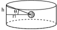
Figure 4: Assumed geometry. An X-ray source (gray sphere) is embodied in a plasma disk expressed as a frame.

We note that the spectral parameters changed between the observations of 1994 and 1995. The luminosity in the 1995 observation was higher than in 1994, and the ratio $N_{\rm Fe\,XXVI}/N_{\rm Fe\,XXV}$ became larger, suggesting that the absorbing matter was more ionized. This behavior is consistent with characteristics of a photo-ionized plasma. Thus, we assume that the source of absorption lines in 1994 and 1995 is a photo-ionized plasma irradiated by the central source. In 1996, the system was considered to be in a different state, because, not only were absorption lines absent, but also the photon index and folding energy of the spectral continuum were different. We calculated electron temperature and ion-population distribution of the photo-ionized plasma with XSTAR (Kallman & Krolik 1996), and searched for parameters which are consistent with those in the high-temperature limit in Table 6. To simplify the calculation, the plasma geometry was assumed to be isotropic around the source. It should be noted that assumption of isotropy is adopted only in the calculation, and that the realistic geometry of the line-absorbing plasma must be anisotropic, since otherwise absorption lines would be canceled by emission lines from out of the line of sight. In the calculations, abundance was assumed to be solar. The absorption-corrected 2–10 keV luminosity was estimated from Table 2 assuming a distance of 12.5 kpc, and used as total luminosity of the model. Continuum spectral parameters were drawn from Table 2. We arbitrarily fixed the ionization parameter $\xi=L/(nr^{2})$ at the innermost boundary of the plasma to be $10^{5.5}$. Our results depend only weakly on this value, because iron and nickel is fully ionized with such a high ionization parameter at the innermost boundary, and thus column density of hydrogen-like or helium-like ions is not sensitive to the innermost condition. The assumed geometry is schematically shown in Fig. 4. We searched a combination of plasma density and outer radius to give $N_{\rm Fe\,XXVI}$ and $N_{\rm Fe\,XXV}$ consistent to observation. The determined parameters are shown in Table 7, and expected column density of ions are shown in Table 8. Obviously, the expected column density of nickel ions in Table 8 is much lower than the observation by one or two orders of magnitude. Therefore, we conclude that the relative abundance of nickel to iron is larger than that of solar value.

We next searched for a combination of plasma parameters to reproduce the column density in the low-temperature limit in Table 6. Since the metal abundance was found to be non-solar, there was no reason to fix them to the solar value. We found that if both the iron and nickel abundances are multiplied by $\sim 100$, the resultant photo-ionized plasma gives the column densities in the low-temperature limit. Other parameters, such as the electron density, the ionization parameter at the outer boundary, and the outer radius of the plasma were hardly affected. Although the column densities are different between the high-temperature-limit and low-temperature-limit cases, the column-density ratios of Fe xxv to Fe xxvi are not much different between the two cases, and thus both yield similar values of $\xi_{1}$. (Subscript“0” and “1” denote values at the innermost and outermost boundary, respectively.) Thus we consider that $\xi_{1}$ and $r_{1}$ in Table 7 are reliable, regardless of the kinematic temperature, the metal abundances, the electron density, or the innermost radius of the plasma.

5.4 Geometry

To produce absorption lines, the solid angle of the line-scattering material from the source must be small, otherwise the absorption lines would be offset by an emission line counterpart. From a moderate assumption that the solid angle is less than $4\pi\exp[-1]$, the disk half thickness, $h$, at the radius $r_{1}$ is constrained as $h/r_{1}\lesssim 0.4$, where $h/r_{1}$ is related to the solid angle as $\Omega=1/\sqrt{1+(h/r_{1})^{2}}$. Therefore, the half opening angle of the plasma, $\theta$, is constrained to be $\theta<20^{\circ}$. The inclination of the jets is $70^{\circ}$ to our line of sight (Mirabel & Rodoríguez 1993). We might reasonably assume that the immediate neighborhood of the central source (e.g., the accretion disk) is also so inclined. From these two constraints, we conclude that the half thickness of the reprocessing plasma is $\sim 0.4r_{1}$. Thus, total mass of the reprocessing plasma is estimated as $\sim 4.4\times 10^{-11}$ M_⊙ (1994) and $\sim 1.5\times 10^{-10}$ M_⊙ (1995).

Note that $n\rm_{p}$ in Table 7 is dependent on assumed geometry and has a large uncertainty, while $\xi_{1}$ and $r_{1}$ are rather model independent and thus reliable. For example, a toroidal plasma distribution around the source can also explain the observed properties, and in this case the path in the plasma along the line of sight will be shorter. Therefore the proton density $n\rm_{p}$ will be larger, conserving column density $(r_{1}-r_{0})\times n_{\rm p}$. The other parameters $\xi_{1}$ and $r_{1}$ would not be changed much, because the former is determined from the ratio $N_{\rm Fe\,XXVI}/N_{\rm Fe\,XXV}$, and the latter is determined from the relation $\xi_{1}=L/(N_{\rm e}r_{1}^{2})$.

5.5 Nature of the Reprocessing Plasma

From the discussion above, we can construct a picture of the plasma producing the absorption lines. It is located at $\sim 10^{11}$ cm from the source, constrained to be within $\theta<20^{\circ}$ of the disk plane, and has a total mass of $10^{-11}$ to $10^{-10}$ M_⊙. The kinetic temperature of iron ion is either high or low. If the metal abundance is comparable to the solar value, then the kinematic temperature must be as high as or higher than 100 keV, which corresponds to a velocity of $\sim 10^{8}$ cm s^-1. If the reprocessing plasma is hotter than 100 keV, it must be observed within 10 s of its production to avoid full ionization of iron and nickel. A post-shock flow within 10 s after the shock is a candidate for such a hot plasma. Both the thermal motion of each ion and the bulk motion of the plasma may give such a high kinematic temperature. An inward or outward bulk flow with a velocity gradient or randomly moving blobs may be the X-ray reprocessor.

As a candidate of such a flow, we suggest a radiation-driven disk wind. If gas at rest exists in the vicinity of the super-Eddington X-ray source, it would be blown out by Thomson scattering. The terminal velocity $v_{\rm wind}$ would be

$$v_{\rm wind}\sim\sqrt{\frac{L\sigma_{\rm Th}}{4\pi rcm_{\rm p}}},$$ (10)

where $L$ is the luminosity of the source, $\sigma_{\rm Th}$ is the cross section of Thomson scattering, $r$ is the initial distance of the gas from the source, and $m\rm_{p}$ is the mass of a proton. If such a gas is supplied from the accretion disk, we would observe a stream with a radial-velocity gradient from 0 to $v_{\rm wind}$. Substituting $r=10^{11}$ cm and $L=4\times 10^{38}$ erg s^-1, a terminal velocity of $v_{\rm wind}=10^{8}$ cm s^-1 is obtained, which coincides with the velocity inferred in the curve-of-growth discussion. It should be noted that most of the centroid energies of the absorption lines in Table 3 are blue-shifted from those in Table 5, which would be expected from the absorption lines from an outward flow with a velocity of $10^{8}$ cm s^-1. Thus a radiation-driven disk wind at $\sim 10^{11}$ cm can well explain the observed absorption line features. Because the disk wind would be refreshed in every $\sim 10^{3}$ s, the outflow rate is estimated as $10^{-7}-10^{-6}$ M_⊙ yr^-1.

On the other hand, if the plasma is very metal rich, the assumption of high-temperature is no longer necessary. The high column density of ions may be explained by low-temperature, metal rich plasma, if the metal abundance is $100$ times higher than the solar value. Even in that case, the conclusion on the geometry of the plasma would not be changed appreciably. The nickel abundance of the jet material of SS 433 has been found to be a few tens times higher than the solar value (Kotani et al. 1997b), which suggests that anomalous abundances may not be rare in binary systems with strong jets. Thus they may be possible that iron and nickel are abundant in the environment of GRS 1915+105, and that the reprocessing plasma has a velocity dispersion smaller than $10^{8}$ cm s^-1 or a lower temperature than 100 keV.

5.6 Alternative situations

In the analysis above, the term of the induced emission $(b_{u}/b_{l})\exp[-h\nu_{0}/kT]$ in equation (3) was neglected. The validity of the assumption can be confirmed as follows. Suppose that a reprocessing plasma is illuminated by an external photon source. An ion in the plasma receives photons with a mean interval of $1/(\sigma_{\rm res}F(\nu_{0}))$, and emits each photon after a time $\sim 1/A_{ul}$, where $F(\nu_{0})$ is the photon flux of the source and $\sigma_{\rm res}$ is the resonant-scattering cross section. Therefore the ratio of the number density of ions at upper state to those at lower state is $\sigma_{\rm res}F(\nu_{0})/A_{ul}$. This is an overestimation because photons at $\nu_{0}$ are reflected by the plasma surface due to resonant scattering. If the ratio is much less than unity, the term of induced emission is negligible. Substituting $\sigma_{\rm res}=c^{2}/(8\pi\nu_{0}^{2})$, the ratio is estimated as

$$\frac{b_{u}}{b_{l}}\exp[-h\nu_{0}/kT]\sim\frac{c^{2}F(\nu_{0})}{8\pi\nu_{0}^{2}A_{ul}}\sim 10^{-10}\left(\frac{L}{10^{39}\rm\;erg\;s^{-1}}\right)\left(\frac{R}{10^{11}\rm\;cm}\right)^{-2},$$ (11)

which is much less than unity. Thus induced emission is shown to be negligible in the case of the photo-ionized plasma treated here.

There is another case where the induced-emission term is important. The ratio  approaches unity on the surface of a neutron star ($R=10^{6}$ cm). Under the presence of the induced emission, more ions are necessary to produce an absorption line. As an estimation of column density of Fe xxvi, we adopt $10^{20.4}$ cm^-2 from Table 6. The corresponding hydrogen column density would be $10^{25}$ cm^-2, assuming solar abundance. To avoid full ionization of iron, the ionization parameter must be $\xi\leq 10^{4}$, and thus the density of the plasma must be $\geq 10^{22}$ cm^-3, and the height of the atmosphere must be $\stackrel{{\scriptstyle<}}{{\sim}}10^{3}$ cm. Although the scale height of the atmosphere at $kT\sim 100$ is larger than $10^{3}$ cm by an order of magnitude, such an atmosphere may produce absorption lines. However, the absorption lines made by the atmosphere would be gravitationally red-shifted, which was not observed. The atmosphere of a neutron star is unlikely to be the origin of the absorption lines. Thus we conclude that induced emission can be neglected in the usual situations where equation (11) is applicable.

6 Summary

Absorption lines of Ca xx K$\alpha$, Fe xxv K$\alpha$, Fe xxvi K$\alpha$, a blend of Ni xxvii K$\alpha$ + Fe xxv K$\beta$, and a blend of Ni xxviii K$\alpha$ + Fe xxvi K$\beta$ have been discovered in the energy spectra of the transient jet source GRS 1915+105. These features can be explained by resonant scattering in a disk-like photo-ionized plasma. From the “curve-of-growth” analysis, column densities of the ions were determined as in Table 6. Adopting the values of high-temperature limit, the physical parameters of the plasma were determined to be:

• outer radius $r_{1}\sim 10^{11}$ cm

• half thickness $h=0.4r_{1}$

• density $n_{\rm p}\sim 10^{11}$ cm^-3

• ionization parameter at the outer boundary of the plasma $\xi=10^{3.8}$

• kinematic temperature of scattering ions $>100$ keV, i.e., $>10^{8}$ cm s^-1, or metal abundance is as large as 100 times of the solar value.

The kinematic temperature of the scattering ions should be very high to account for the observed large equivalent widths of the absorption lines, if solar abundance is assumed. If the temperature is so high, the plasma may not be in equilibrium, with an ionization temperature lower than the kinematic temperature. Thus the high kinematic temperature may be explained by a bulk motion, such that a velocity difference up to $\sim 10^{8}$ cm s^-1 within the plasma flow, or perhaps plasma blobs moving randomly. We found that a radiation-driven accretion flow with a mass outflow rate of $10^{-7}-10^{-6}$ M_⊙ yr^-1 can account for the absorption lines. Alternatively, if the plasma is extremely metal rich, such a high kinematic temperature is not necessary. Regardless of the kinematic temperature, we concluded from the observed iron to nickel abundance ratios that the abundances are non-solar.

We thank Craig Markwardt for careful reading of the manuscript.

Appendix A. Pile-up correction

The SIS/ASCA suffers pileup when observing a bright source $\stackrel{{\scriptstyle>}}{{\sim}}$ 100 counts s^-1. If two or more photons fall on a single pixel or neighboring pixels (Moore neighbor) on a CCD chip of the SIS within the same readout period, they are recognized as a single photon by the on-board event-detection algorithm, and their energies are summed to make a single pulse height. This phenomenon is called “pileup” and causes a decrease in the photon counting rate and hardening of the spectrum. In observations of bright sources, pileup is non-negligible and correction is necessary for precise spectral analysis. We have developed a new code for this purpose. This code also can cope with attitude fluctuations of the satellite, which were in fact significant during the GRS 1915+105 observation in 1994.

Our code simulates the pileup using the observed events as the seeds. First, the source position is determined on the CCD image without correction, and the image core where the counting rate is higher than a certain threshold is discarded from further analysis. The threshold was empirically determined to be 0.023 counts pixel^-1 readout^-1, above which we found the pileup effect was so significant that uncorrectable. The pixels on the CCD chip are divided into several annuli centered at the source. The annuli widths are determined so that the counting rate per pixel within each annulus is almost uniform. The number of detected events in the $i$-th annulus and the $j$-th readout is defined as $a_{ij}$. By dividing the chips into annuli, both the count rate and the image are eventually recovered.

Next, the temporal order of all the $N_{i}=\Sigma_{j}a_{ij}$ events in the $i$-th annulus is randomized, while each event retains its position, pulse-height, and charge-distribution pattern, i.e., grade information. The event series before and after randomization are denoted as

$$\gamma_{i1},\;\gamma_{i2},\;\ldots\;,\gamma_{i\,N_{i}}$$ (12)

and

$$\gamma_{i\sigma(1)},\;\gamma_{i\sigma(2)},\;\ldots\;,\gamma_{i\sigma(N_{i})},$$ (13)

where $\sigma(k)$ is a randomizing function which returns an integer between 1 and $N_{i}$, and satisfies $\sigma(k)\neq\sigma(l)$ if $k\neq l$. For each read-out, the randomized events are injected on a virtual CCD chip, and the same event detection algorithm as that on-board is applied (Gendreau 1995). For example, to simulate the $j$-th readout of the $i$-th ring, a series of events

$$\gamma_{i\sigma(\Sigma_{k=1}^{j-1}a_{ik}+1)},\;\gamma_{i\sigma(\Sigma_{k=1}^{j-1}a_{ik}+2)},\;\ldots\;,\gamma_{i\sigma(\Sigma_{k=1}^{j}a_{ik})}$$ (14)

is created (note that $\Sigma_{k=1}^{j}a_{ik}-\Sigma_{k=1}^{j-1}a_{ik}=a_{ij}$), and charge-distribution patterns on the virtual CCD chip are calculated from the position, pulse-height, and original charge-distribution pattern or grade of each input event. If the SIS observation mode is BRIGHT and the information on split charge has been lost, the charge is assumed to be 40 ADU (the split-threshold). The spectrum of the injected events is recorded as $f_{2}(E)$. If there is no pileup, all $a_{ij}$ events should be detected. On the other hand, the detected events may be less than $a_{ij}$ if pileup is accounted for. In that case additional events are randomly picked up from the total $N_{i}$ events and injected onto the virtual chip (also added to $f_{2}(E)$) until $a_{ij}$ events are detected. When the number of detected events has reached $a_{ij}$, the spectrum determined by the event detection algorithm is recorded as $f_{3}(E)$, which will be the simulated spectrum affected by the pileup. This procedure is repeated for all the annuli and readouts. It should be noted that all the original events are used in the whole process at least once. By using all the events, fluctuations caused by random pick up will be reduced to minimum. Finally, the pure pileup spectrum $f_{4}(E)$ and resultant pileup-corrected spectrum $f_{5}(E)$ are estimated as

$$f_{4} = f_{3}-f_{2}$$ (15)

$$f_{5} = f_{1}-f_{4}=f_{1}+f_{2}-f_{3},$$ (16)

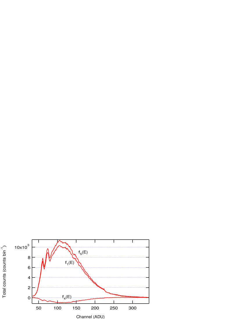
Figure 5: Spectrum before and after pile-up correction. The Sensor-0 Chip-1 data of 1994 are presented as an example. The observed spectrum before correction $f_{1}(E)$, the calculated pure pileup component $f_{4}(E)$, and the resultant pileup-corrected spectrum $f_{5}(E)$ are shown. Energy is expressed in analog-to-digital-converter units (ADU), and the range is between 0.5–10 keV. In the lower energy band (50–200 ADU), photons are lost by pileup and thus $f_{4}(E)$ is negative by definition. In the higher energy band ($>$ 250 ADU), pseudo photons are made by pileup. Although it is difficult to discern by eye in a linear plot, the effect in the higher band is not negligible.

where $f_{1}(E)$ is the observed spectrum before the correction. In Fig. 5, an example of the pileup correction is exhibited.

Table 1: Observation log

No.	Start	End	Exposure Time	SIS Mode
	(UT)	(UT)	(ks)
1	1994/09/27 00:40	1994/09/27 13:00	10	BRIGHT
2	1995/04/20 09:50	1995/04/20 22:40	16	FAINT
3	1996/10/23 02:40	1996/10/23 18:20	11	BRIGHT
4	1997/04/25 08:10	1997/04/25 21:00	20	BRIGHT
5	1998/04/04 16:20	1998/04/05 03:30	20	BRIGHT
6	1999/04/15 20:10	1999/04/16 15:00	20	BRIGHT

Table 2: Best-fit parameters of the GIS spectral continuum

No.	$N_{\rm H1}$	$f$	$N_{\rm H2}$	$A$	$E_{\rm fold}$	$\Gamma$	$\chi^{2}_{\nu}$ ($\nu$)
	($10^{22}$ cm-2)		($10^{22}$ cm-2)		(keV)
1	$2.97^{+0.10}_{-0.10}$	$0.551^{+0.040}_{-0.040}$	$55^{+6}_{-5}$	$4.67^{+0.44}_{-0.41}$	$1.28^{+0.04}_{-0.04}$	$-0.91^{+0.13}_{-0.13}$	1.13 (131)
2	$3.46^{+0.10}_{-0.10}$	$0.563^{+0.065}_{-0.070}$	$81^{+10}_{-10}$	$5.84^{+0.69}_{-0.60}$	$1.35^{+0.05}_{-0.05}$	$-1.18^{+0.13}_{-0.13}$	1.13 (131)
3	$4.75^{+0.07}_{-0.04}$	$0.219^{+0.066}_{-0.045}$	$71^{+22}_{-14}$	$17.6^{+1.4}_{-1.2}$	$4.61^{+0.28}_{-0.27}$	$1.50^{+0.07}_{-0.08}$	1.12 (174)

Table 3: Best-fit parameters of the feature around iron-K absorption

Model Component	Parameter	1994	1995
Emission Line	Energy (keV)	$6.484^{+0.044}_{-0.045}$	$\cdots$
	Width (eV)	0 (fixed)	$\cdots$
	EW (eV)	$15.8^{+6.3}_{-6.9}$	$\cdots$
Negative Gaussian A	Energy (keV)	$6.720^{+0.015}_{-0.017}$	$6.690^{+0.028}_{-0.034}$
	Width (eV)	$<39$	$<89$
	EW (eV)	$35.8^{+3.7}_{-7.8}$	$27.5^{+4.7}_{-6.3}$
Negative Gaussian B	Energy (keV)	$7.000^{+0.020}_{-0.014}$	$6.964^{+0.012}_{-0.024}$
	EW (eV)	$43.2^{+6.3}_{-5.3}$	$48.3^{+5.4}_{-5.7}$
Negative Gaussian C	Energy (keV)	$7.843^{+0.037}_{-0.035}$	$7.839^{+0.043}_{-0.037}$
	EW (eV)	$30.8^{+11.2}_{-5.8}$	$29.9^{+8.4}_{-8.5}$
Negative Gaussian D	Energy (keV)	$8.199^{+0.065}_{-0.064}$	$8.181^{+0.060}_{-0.057}$
	EW (eV)	$22^{+11}_{-12}$	$19^{+9}_{-10}$
Absorption Edge	Energy (keV)	$\cdots$	7.117 (fixed)
	Max. Opt. Depth	$\cdots$	$0.122^{+0.027}_{-0.027}$
$\chi^{2}_{\nu}$ ($\nu$)		1.03 (56)	1.05 (57)

Table 4: Best-fit parameters of the absorption features at 4 keV

Model Component	Parameter	1994	1995
Negative Gaussian X	Energy (keV)	$4.071^{+0.068}_{-0.097}$	$4.05^{+0.11}_{-0.11}$
	Width (eV)	$<210$	10 (fixed)
	EW (eV)	$10.2^{+7.5}_{-5.4}$	$<7.9$
$\chi^{2}_{\nu}$ ($\nu$)		0.80 (56)	1.24 (57)

Table 5: Absorption-line candidates

Ion	Upper Level	Energy	Oscillator Strength	Einstein Coefficient
		(keV)		(s-1)
Fe xxv	$1s^{1}2p^{1}$ $\rm{}^{3}P_{1}$	6.6684925 (1)	0.0687 (1)	$4.42\times 10^{13}$
Fe xxv	$1s^{1}2p^{1}$ $\rm{}^{1}P_{1}$	6.7011266 (1)	0.703 (1)	$4.57\times 10^{14}$
Fe xxvi	$2p^{1}$ $\rm{}^{2}P_{1/2,3/2}$	6.9519639, 6.9731781 (3)	0.44 (4)	$1.5\times 10^{14}$
Ni xxvii	$1s^{1}2p^{1}$ $\rm{}^{3}P_{1}$	7.7668938 (1)	0.0883 (1)	$7.70\times 10^{13}$
Ni xxvii	$1s^{1}2p^{1}$ $\rm{}^{1}P_{1}$	7.8062340 (1)	0.683 (1)	$6.02\times 10^{14}$
Fe xxv	$1s^{1}3p^{1}$ $\rm{}^{1}P_{1}$	7.8820244 (2)	0.138 (2)	$1.24\times 10^{14}$
Ni xxviii	$2p^{1}$ $\rm{}^{2}P_{1/2,3/2}$	8.0731039, 8.1017429 (3)	0.44 (4)	$2.07\times 10^{14}$
Fe xxvi	$3p^{1}$ $\rm{}^{2}P_{1/2,3/2}$	8.2636944, 8.2526875 (3)	0.046 (4)	$2.3\times 10^{13}$

Table 6: Column density of absorbing ions

	High-Temperature Limit ($kT=1000$ keV)
	Fe xxv	Fe xxvi	Ni xxvii	Ni xxviii
1994	$17.7^{+0.1}_{-0.1}$	$18.0^{+0.1}_{-0.1}$	$17.5^{+0.2}_{-0.2}$	$17.6^{+0.3}_{-0.7}$
1995	$17.6^{+0.1}_{-0.1}$	$18.1^{+0.1}_{-0.1}$	$17.5^{+0.2}_{-0.2}$	$17.4^{+0.5}_{-0.9}$
	Low-Temperature Limit ($kT=0.1$ keV)
	Fe xxv	Fe xxvi	Ni xxvii	Ni xxviii
1994	$19.3^{+0.1}_{-0.2}$	$20.3^{+0.1}_{-0.1}$	$18.8^{+0.4}_{-0.3}$	$19.4^{+0.5}_{-1.2}$
1995	$19.0^{+0.1}_{-0.2}$	$20.4^{+0.1}_{-0.1}$	$18.8^{+0.3}_{-0.4}$	$19.1^{+0.8}_{-1.5}$

Table 7: Parameters of the photo-ionized plasma

	$L$	$\xi_{0}$	$r_{0}$	$\xi_{1}$	$r_{1}$	$n\rm_{p}$
	(erg s-1)	(erg s-1 cm)	(cm)	(erg s-1 cm)	(cm)	(cm-3)
1994	$4.0\times 10^{38}$ (fixed)	$10^{5.5}$ (fixed)	$9\times 10^{10}$	$10^{3.8}$	$6\times 10^{11}$	$1.5\times 10^{11}$
1995	$8.8\times 10^{38}$ (fixed)	$10^{5.5}$ (fixed)	$14\times 10^{10}$	$10^{3.8}$	$9\times 10^{11}$	$1.5\times 10^{11}$

Calculated from ionization parameter $\xi$, and not a free parameter.

Table 8: Model prediction of ion column density

	H ii	O viii	Si xiv	S xvi	Ca xx	Fe xxv	Fe xxvi	Ni xxvii	Ni xxviii
1994	22.9	16.1	15.9	16.0	15.9	17.7	18.0	15.1	16.7
1995	23.1	16.4	16.0	16.1	15.9	17.6	18.1	16.7	16.9

(a) 1994 September

(b) 1995 April

(c) 1996 October

Figure 1: GIS Spectra. (a) 1994 September, (b) 1995 April, and (c) 1996 October. Observed data (cross), best-fit model (histogram), and residuals (bottom panel) are plotted. Each error bar includes systematic uncertainties of 2 %. The data of GIS-2 and GIS-3 were combined. Dead time and telemetry saturation were not corrected. The energy range 6–8 keV in the data of 1994 and 1995 was excluded in fitting. The structure at 4.7 keV is due to an instrumental Xe-L edge.

(a) 1994 September

(b) 1995 April

(c) 1996 October

Figure 2: SIS Spectra. (a) 1994 September, (b) 1995 April, and (c) 1996 October. Observed data (cross), best-fit model (histogram), residuals (crosses in lower panel), and residuals for the model without absorption lines (solid line in lower panel) are plotted. Absorption features are clearly seen in the solid curve. As for the data of 1994 and 1995, only the range around the iron absorption features are plotted, while the overall spectrum is plotted for 1996. The data of SIS-0 and SIS-1 were combined. The structure around 2–2.5 keV is instrumental.

(a) Fe xxv K$\alpha$

(b) Fe xxvi K$\alpha$

(c) Fe xxv K$\beta$

(d) Fe xxvi K$\beta$

(e) Ni xxvii K$\alpha$

(f) Ni xxviii K$\alpha$

Figure 3: Curves of growth. (a) Fe xxv K$\alpha$, (b) Fe xxvi K$\alpha$, (c) Fe xxv K$\beta$, (d) Fe xxvi K$\beta$, (e) Ni xxvii K$\alpha$, and (f) Ni xxviii K$\alpha$. The curves in each panel correspond to kinematic temperature of 1000 keV, 100 keV, 10 keV, 1 keV, and 0.1 keV, from high to low.

Erratum: “ASCA Observations of the Absorption-Line Features from the Super-Luminal Jet Source GRS 1915+105” (ApJ, 539, 413 [2000])

We have discovered errors in the calculation of some of the Einstein coefficients in Table 5 and some plots in Figure 3. Due to the errors, the square-root section of the curves of growth of Fe xxvi K$\alpha$ and K$\beta$, and Ni xxviii K$\alpha$ in Figure 3 were a few times underestimated. We correct Table 5 and re-plot Figure 3 together with the unaffected curves. We thank Aya Kubota and Chirs Done for pointing out this error.

TABLE 5

Absorption-line candidates Ion Upper Level Energy Oscillator Strength Einstein Coefficient (keV) (s^-1) Fe xxv $1s^{1}2p^{1}$ $\rm{}^{3}P_{1}$ 6.6684925 (1) 0.0687 (1) $4.42\times 10^{13}$ Fe xxv $1s^{1}2p^{1}$ $\rm{}^{1}P_{1}$ 6.7011266 (1) 0.703 (1) $4.57\times 10^{14}$ Fe xxvi $2p^{1}$ $\rm{}^{2}P_{1/2,3/2}$ 6.9519639, 6.9731781 (3) 0.44 (4) $3.1\times 10^{14}$ Ni xxvii $1s^{1}2p^{1}$ $\rm{}^{3}P_{1}$ 7.7668938 (1) 0.0883 (1) $7.70\times 10^{13}$ Ni xxvii $1s^{1}2p^{1}$ $\rm{}^{1}P_{1}$ 7.8062340 (1) 0.683 (1) $6.02\times 10^{14}$ Fe xxv $1s^{1}3p^{1}$ $\rm{}^{1}P_{1}$ 7.8820244 (2) 0.138 (2) $1.24\times 10^{14}$ Ni xxviii $2p^{1}$ $\rm{}^{2}P_{1/2,3/2}$ 8.0731039, 8.1017429 (3) 0.44 (4) $4.1\times 10^{14}$ Fe xxvi $3p^{1}$ $\rm{}^{2}P_{1/2,3/2}$ 8.24636944, 8.2526875 (3) 0.046 (4) $4.5\times 10^{13}$

Fig. 3a                                      Fig. 3b

Fig. 3c                                      Fig. 3d

Fig. 3e                                      Fig. 3f

Fig. 3—Curves of growth. (a) Fe xxv K$\alpha$, (b) Fe xxvi K$\alpha$, (c) Fe xxv K$\beta$, (d) Fe xxvi K$\beta$, (e) Ni xxvii K$\alpha$, and (f) Ni xxviii K$\alpha$. The curves in each panel correspond to kinematic temperature of 1000 keV, 100 keV, 10 keV, 1 keV, and 0.1 keV, from high to low.

This figure replaces Fig. 3 of the original manuscript. The square-root section of the curves in Fig. 3b, 3d, and 3f are a few times increased by this correction. The unaffected figures, 3a, 3c, and 3e are also shown.

References

- (1) Belloni, T., Mendez, M., King, A. R., Van Der Klis, M. & Van Paradijs, J. 1997, ApJ, 479, L145
- (2) Castro-Tirado, A. J., Brandt, S., & Lund, N. 1992, IAUC, 5590
- (3) Drake, G. W. F. 1979, Phys. Rev. A, 19, 1387
- (4) Ebisawa, K. 1997a, in X-Ray Imaging and Spectroscopy of Cosmic Hot Plasmas, ed. F. Makino & K. Mitsuda (Tokyo; Universal Academy Press), 427
- (5) Ebisawa, K. 1997b, in All-Sky X-Ray Observations in the Next Decade, ed. M. Matsuoka & N. Kawai (Saitama; RIKEN), 69
- (6) Ebisawa, K., Ueda, Y., Inoue, H., Tanaka, Y., & White, N. E. 1996, ApJ, 467, 419
- (7) Ebisawa, K., Takeshima, T., White, N. E., Kotani, T., Dotani, T., Ueda, Y., Harmon, B. A., Robinson, C. R., et al. 1998, in IAU Symp., 188, The Hot Universe, ed. K. Koyama, S. Kitamoto, & M. Itoh (Dordrecht; Kluwer Academic Publishers), 392
- (8) Gendreau, K. C., 1995, Ph. D Thesis, MIT
- (9) Hjellming, R. M., & Rupen, M. P. 1995, Nature, 375, 464
- (10) Lin, C. D., Johnson, W. R., & Dalgarno, A. 1977, ApJ, 217, 1011
-
(11)
Kallman, T.R., & Krolik J.H., XSTAR User’s
Guide Version 1.27,
ftp://legacy.gsfc.nasa.gov/software/plasma_codes/xstar (1996). - (12) Kotani, T., Kawai, N., Matsuoka, M., Dotani, T., Inoue, H., Nagase, F., Tanaka, Y., Ueda, U., et al. 1997a, in The Proceedings of the Fourth Compton Symposium, ed. C. D. Dermer, M. S. Strickman, & J. D., Kurfess (New York; American Institute of Physics), 922
- (13) Kotani, T., Kawai, N., Matsuoka, M., & Brinkmann, W. 1997b, in X-Ray Imaging and Spectroscopy of Cosmic Hot Plasmas, ed. F. Makino & K. Mitsuda (Tokyo; Universal Academy Press, Inc.), 443
- (14) Kotani, T., Ebisawa, K., Inoue, H., Nagase, N., Ueda, Y. 1999a, in Proceedings of 3rd INTEGRAL Workshop, Extreme Universe, in press
- (15) Kotani, T., Ebisawa, K., Inoue, H., Kawai, N., Matsuoka, M., Nagase, F., Robinson, C. R., Takeshima, T., et al. 1999b, Advances in Sp. Research, in press
- (16) Makishima, K., et al. 1996, PASJ, 48, 171
- (17) Mewe, R., Gronenschild, E. H. B. M., & van den Oord, G. H. J. 1985, A&AS, 62, 197
- (18) Mirabel, I. F., Dhawan, V., Chaty, S., Rodriguez, L. F., Marti, J., Robinson, C. R., Swank, J. & Geballe, T. 1998, A&A, 330, L9
- (19) Mirabel, I. F., & Rodríguez, L. F. 1994, Nature, 371, 46
- (20) Mirabel, I. F., & Rodríguez, L. F. 1996, in Solar and Astrophysical Magnetohydrodynamic Flows, ed. K. C. Tsinganos (Dordrecht; Kluwer Academic Publishers), 683
- (21) Mitsuda, K., et al. 1984, PASJ, 36, 741
- (22) Nagase, F., Inoue, H., Kotani, T., & Ueda, Y. 1994, IAUC, 6094
- (23) Ohashi, T., et al. 1996, PASJ, 48, 157
- (24) Rybicki, G. B. & Lightman, A. P. 1979, Radiative Processes in Astrophysics (John Wiley & Sons, Inc., Toronto)
- (25) Sazonov, S., Sunyaev, R., Alexandrovich, N., & Borozdin, K. 1994, IAUC, 6080
- (26) Serlemitsos, P. J., et al. 1995, PASJ, 47, 105
- (27) Spitzer, Jr., L. 1978, Physical Processes in the Interstellar Medium (Toronto; John Wiley & Sons, Inc.)
- (28) Sugar, J., & Corliss, C. 1985, J. Phys. Chem. Ref. Data, 14, Supplement No. 2
- (29) Yamashita, A., et al. 1997, IEEE Transaction on Nucl. Sci., 44, 847
- (30) Ueda, Y., Inoue, H., Tanaka, Y., Ebisawa, K., Nagase, F. & Kotani, T. 1997, in All-Sky X-Ray Observations in the Next Decade, ed. M. Matsuoka & N. Kawai (Saitama; RIKEN), 141
- (31) Ueda, Y., Inoue, H., Tanaka, Y., Ebisawa, K., Nagase, F., Kotani, T., & Gehrels, N. 1998, ApJ, 492, 782; 1998, ApJ, 500, 1069 (Erratum)