Using HI to probe large scale structures at $z\sim 3$ .

Abstract

The redshifted $1420\,\rm MHz$ emission from the HI in unresolved damped Lyman-$\alpha$ clouds at high z will appear as a background radiation in low frequency radio observations. This holds the possibility of a new tool for studying the universe at high-$z$, using the mean brightness temperature to probe the HI content and its fluctuations to probe the power spectrum. Existing estimates of the HI density at $z\sim 3$ imply a mean brightness temperature of $1\,{\rm mK}$ at $320\,{\rm MHz}$. The cross-correlation between the temperature fluctuations across different frequencies and sight lines is predicted to vary from $10^{-7}\,\rm K^{2}$ to $10^{-8}\,\rm K^{2}$ over intervals corresponding to spatial scales from $10\,{\rm Mpc}$ to $40\,{\rm Mpc}$ for some of the currently favoured cosmological models. Comparing this with the expected sensitivity of the GMRT, we find that this can be detected with $\sim 10\,\rm hrs$ of integration, provided we can distinguish it from the galactic and extragalactic foregrounds which will swamp this signal. We discuss a strategy based on the very distinct spectral properties of the foregrounds as against the HI emission, possibly allowing the removal of the foregrounds from the observed maps.

1 Introduction

The problem of determining the distribution of matter on large scales in the universe and understanding the large scale structure (LSS) formation is of prime importance in modern cosmology. Observing the angular positions and redshifts of galaxies has been the most straightforward method of mapping the LSS in the present day universe (Peebles 1993, Peebles 1980), but the interpretation of these observations is complicated by the fact that the relation between the distribution of galaxies and the distribution of underlying matter is not fully understood (Bardeen et al.  1986). Other direct methods use galaxy clusters or super-clusters as tracers to map the large scale structures. A large variety of techniques have been developed and applied to quantify the distribution of galaxies, and amongst these the correlation functions (two-, three-point correlation functions, etc) and their Fourier counterparts (power spectrum, bi-spectrum, etc.) have been most popular (Peebles 1980). Much of the work comparing the observations with different theories has been based on these.

An alternative approach is to use observations of fluctuations in the diffuse extragalactic background radiation at different wavelengths to probe the large scale structure. Here, the observations of anisotropies in the cosmic microwave background radiation (CMBR) have been most important. These observations probe the clustering of matter at the last scattering surface (e.g. Bond 1996), and combined with the information from the galaxy surveys, they have been successful in narrowing down the allowed class of theoretical models of LSS formation (e.g., Peacock 1999 and reference therein). The study of diffuse background at other wavelengths has been used to infer the clustering properties of matter at more recent epochs. Shectman (1974) observed fluctuations in the optical background; the results of this observation are consistent with predictions from galaxy counts (Peebles 1980). This method has also been applied to far-infrared background (Kashlinsky et al. 1997) and recently the first detection of fluctuations in this background has been reported (Kashlinsky et al. 1999). Gorjian, Wright and Chary (1999) have recently reported a tentative detection of a near-infrared background. There are similar predictions for fluctuations in the X-ray background (Barcons et al.  2000, Barcons et al.  1998).

In this paper we investigate the possibility of using the extragalactic background radiation at low radio frequencies (meter wave) to probe the LSS. This is largely motivated by the fact that the Giant Meter-wave Radio Telescope (GMRT; Swarup et al.  1991) which is designed to observe in several frequency bands in the interval $150\,{\rm MHz}$ to $1420\,{\rm MHz}$ has recently started functioning. This frequency range corresponds to the $1420{\rm MHz}$ emission from HI in the redshift range $0\leq z\leq 8.5$. Absorption studies along sight lines to quasars indicate that most of the HI in the redshift range $0\leq z\leq 3$ is in damped Lyman-$\alpha$ (DLA) clouds and the density of HI in DLAs has been determined reasonably well from absorption studies (Lanzetta, Wolfe, & Turnshek 1995). Although the HI emission from individual DLAs at high $z$ is too faint to detect using presently available telescopes, the redshifted HI emission from unresolved DLAs will contribute to the background radiation at low frequencies. In this paper we investigate how the brightness temperature of this radiation is related to the density and peculiar velocity of the HI. We consider the possibility of detecting correlations in the fluctuations in this component of the background radiation and using this to probe LSS at high $z$.

The possibility of observing the redshifted 21 cm emission from HI at high $z$ has been discussed earlier by many authors in a large variety of contexts. One of the first papers (Sunyaev & Zel’dovich, 1975) considers the possibility of meter-wave observations to detect protogalaxies and protoclusters at $z\leq 10$. There have been several attempts to detect the HI in proto-clusters and proto-super clusters (see Subrahmanyan & Anantharamaiah 1990 and reference therein).

More recently Subramanian and Padmanabhan (1993) have calculated the abundance of protoclusters as a function of the redshifted HI flux density for various redshifts for both the CDM and HDM models. In a later paper Kumar, Padmanabhan and Subramanian (1995) have calculated the line profile of the HI emission from a spherically symmetric protocluster. Bagla, Nath and Padmanabhan (1997) and Bagla (1998) have used a combination of N-body simulations and a model for the behaviour of the baryons to calculate the abundance and the expected flux from the HI in structures like protoclusters at high redshifts. A major uncertainty in all of these works is in the assumptions about the HI content of the universe at high redshifts. The main focus of all of these works has been on individual peaks of the density fluctuations (protoclusters) which will manifest themselves as detectable features in low-frequency radio maps. Subramanian and Padmanabhan (1993) have also studied the possibility of detecting the excess variance in radio images due to the density fluctuations in the HI at high $z$.

Katz, Weinberg and Hernquist (1998) have used smoothed particle hydrodynamic simulations to study the distribution of HI gas at high $z$ and they consider the possibility of detecting HI emission from galaxies at $z>2$.

Tozzi et al.  (1999) and Shaver et al.  (1999) have studied the possibility of detecting the HI in the IGM at $z>5$. The state of the HI at these redshifts is unknown and these works are based on different scenarios for the reionization of the universe.

The work presented here differs significantly from the previous papers in that:

• It is restricted to $z<3.5$ where the HI content of the universe is well determined from DLA absorption studies. We use the results of these observations as inputs to our calculations.

• Instead of looking at the possibility of detecting individual features (as has been the focus of a large number of previous papers) we have studied the statistical properties of the fluctuations in the brightness temperature in low frequency radio maps. The statistical quantity we have studied is the cross-correlation between the temperature fluctuations along different lines of sight in radio map made at different frequencies. Individual features corresponding to protoclusters are rare events and protoclusters with flux in the range $1.5-3\,{\rm m\,Jy}$ are predicted to occur with abundances in the range $10^{-8}-10^{-7}\,{\rm Mpc}^{-3}$ in the CDM model (Subramanian and Padmanabhan, 1993). Even small density fluctuations will contribute to the cross-correlation signal and our proposal has the advantage of simultaneously using the signal in all the pixels in all the frequency channels across the bandwidth of observation.

The structure of the paper is as follows: in §2 we discuss the basic formalism of calculating the brightness temperature and fluctuations in the redshifted 21 cm radiation, in §3 we discuss the numerical results for two currently favoured cosmological models. In §4, the observational difficulties in the presence galactic and extragalactic foregrounds are presented, and we discuss a possible strategy for overcoming these. §5 gives a summary of our main results.

2 Formalism.

We treat the HI in damped Lyman-$\alpha$ (DLA) systems as a continuous distribution with $n_{\rm HI}(\boldsymbol{x},t)$ denoting the comoving number density of HI atoms in the excited state of the hyperfine transition. Such a treatment is justified in a situation where the resolution of the observations is not sufficient to detect individual DLAs. In addition, the fact that the HI actually does not have a continuous distribution but is distributed in discrete objects can, if required. be taken into account when calculating statistical measures of the fluctuation in the HI distribution.

The HI emission which is at a frequency $\nu_{e}=1420{\rm MHz}$ in the rest frame of the gas it is emitted from is redshifted to a frequency $\nu$ for an observer located at the origin of the coordinate system. Taking into account the effects of both the expansion of the universe as well as the peculiar velocity $\boldsymbol{v}(\boldsymbol{x},t)$ of the HI at the time of emission and $\boldsymbol{v}(0,t_{0})$ of the observer at the present time, the comoving coordinate $\boldsymbol{x}$ of the HI and $\nu$ are related by

$$\boldsymbol{x}=\boldsymbol{n}\,c\int_{\frac{\nu}{\nu_{e}(1-W)}}^{1}\frac{d\,a}{a^{2}H(a)}$$ (1)

in a spatially flat universe. Here $\boldsymbol{n}=\boldsymbol{x}/x$ is a unit vector along the line of sight to the HI, $W(\boldsymbol{x})=\boldsymbol{n}\cdot[\boldsymbol{v}(\boldsymbol{x},t)-\boldsymbol{v}(0,t_{0})]/c$ accounts for the effects of the peculiar velocities and

$$H(a)=\frac{\dot{a}(t)}{a(t)}=H_{0}\sqrt{\Omega_{m0}a^{-3}+\lambda_{0}}$$ (2)

is the Hubble parameter at the epoch when the scale factor has value $a$.

When discussing observations of the redshifted HI emission, it is convenient to use ${\boldsymbol{\nu}}=\boldsymbol{n}\nu$ to simultaneously denote the frequency and the direction of the observation. The vector $\boldsymbol{\nu}$ fixes both the comoving position $\boldsymbol{x}$ of the HI from where the radiation originates and the time $t$ at which the radiation originates, and we shall use $\boldsymbol{\nu}$ and $(\boldsymbol{x},t)$ interchangeably. Here we calculate how $T(\boldsymbol{\nu})$ the brightness temperature of the radiation is related to the density $n_{\rm HI}(\boldsymbol{x},t)$ and the the peculiar velocity $\boldsymbol{v}(\boldsymbol{x},t)$ of the HI.

The energy flux in the frequency interval $d^{3}\nu$ can be calculated if we know the number of excited HI atoms in the comoving volume $d^{3}x$ from where the radiation originates and it is given by

$${\rm Flux}=\frac{h_{P}\,\nu_{e}\,A_{21}\,n_{\rm HI}(\boldsymbol{x},t)\,d^{3}x}{4\,\pi\,r^{2}_{L}(\boldsymbol{x})}$$ (3)

Here $r_{L}$ is the luminosity distance which is given by

$$r_{L}(\boldsymbol{x})=x\,[1-W]\,\frac{\nu_{e}}{\nu}$$ (4)

The flux is also related to the specific intensity as follows

$${\rm Flux}=\frac{I(\boldsymbol{\nu})}{\nu^{2}}d^{3}\nu$$ (5)

which allows us to calculate the specific intensity to be

$$\frac{I(\boldsymbol{\nu})}{\nu^{2}}=\frac{h_{P}\,\nu_{e}\,A_{21}\,n_{\rm HI}(\boldsymbol{\nu})}{4\,\pi\nu_{e}^{2}}\left\{\frac{1}{[1-W(\boldsymbol{\nu})]}\frac{\nu}{x}\right\}^{2}\left|\frac{\partial\boldsymbol{x}}{\partial\boldsymbol{\nu}}\right|\,.$$ (6)

where $|\frac{\partial\boldsymbol{x}}{\partial\boldsymbol{\nu}}|$ is the Jacobian of the transformation from $\boldsymbol{\nu}$ to $\boldsymbol{x}$ given in equation (1).

It should be noted here that the effect of the peculiar velocity $(i.e.W)$ can be neglected if we restrict the analysis to scales which are much smaller than the horizon. This is not true for the spatial derivatives of the peculiar velocities which appears in the Jacobian and we retain such terms in our analysis. Calculating the Jacobian gives us

$$\left|\frac{\partial\boldsymbol{x}}{\partial\boldsymbol{\nu}}\right|=\left(\frac{x}{\nu}\right)^{2}\frac{c}{H(\frac{\nu}{\nu_{e}})}\frac{\nu_{e}}{\nu^{2}}\left[1-\frac{\nu_{e}}{\nu}\frac{(\boldsymbol{n}\cdot\boldsymbol{\nabla})(\boldsymbol{n}\cdot\boldsymbol{v})}{H(\frac{\nu}{\nu_{e}})}\right]\,.$$ (7)

Equations (6) and (7) allows us to calculate the brightness temperature of the radiation

$$T(\boldsymbol{\nu})=\left(\frac{c^{2}}{2k_{B}}\right)\frac{I(\boldsymbol{\nu})}{\nu^{2}}$$ (8)

which gives us

$$T(\boldsymbol{\nu})=\frac{T_{21}N_{21}(\boldsymbol{\nu})}{8\pi}\frac{A_{21}}{H(\frac{\nu}{\nu_{e}})}\left(\frac{\nu_{e}}{\nu}\right)^{2}\left[1-\frac{\nu_{e}}{\nu}\frac{(\boldsymbol{n}\cdot\boldsymbol{\nabla})(\boldsymbol{n}\cdot\boldsymbol{v})}{H(\frac{\nu}{\nu_{e}})}\right]\,.$$ (9)

where $T_{21}=h_{p}\nu_{e}/k_{B}$ and $N_{21}(\boldsymbol{\nu})=(c/\nu_{e})^{3}\,n_{HI}(\boldsymbol{\nu})$ is the number of HI atoms in the excited state in a comoving volume $(21{\rm cm})^{3}$.

The number density $n_{\rm HI}(\boldsymbol{\nu})$ can be written as a sum of two parts, namely the mean $\bar{n}_{HI}(\nu)$ and the fluctuation $\Delta n_{HI}(\boldsymbol{\nu})$. We assume that the fluctuation in the number density of HI can be related to the perturbations in the underlying dark matter distribution $\delta(\boldsymbol{\nu})$ through a time dependent linear bias parameter $b(\nu)$ which gives us

$$N_{21}(\boldsymbol{\nu})=\bar{N}_{21}(\nu)[1+b(\nu)\delta(\boldsymbol{\nu})]\,.$$ (10)

We use this to calculate the isotropic part of the temperature

$$\bar{T}(\nu)=\frac{2.38\,{\rm K}h^{-1}\,\bar{N}_{21}(\nu)}{\sqrt{\Omega_{m0}(\frac{\nu_{e}}{\nu})^{3}+\lambda_{0}}}\left(\frac{\nu_{e}}{\nu}\right)^{2}$$ (11)

and the fluctuation

$$\Delta T(\boldsymbol{\nu})=\bar{T}(\nu)\left[b(\nu)\delta(\boldsymbol{\nu})-\frac{\nu_{e}}{\nu}\frac{(\boldsymbol{n}\cdot\boldsymbol{\nabla})(\boldsymbol{n}\cdot\boldsymbol{v})}{H(\frac{\nu}{\nu_{e}})}\right]$$ (12)

Now, in the linear theory of density perturbations, both the perturbation and the peculiar velocity can be expressed in terms of a potential i.e.

$$\delta(\boldsymbol{x},t)=D(t)\nabla^{2}\psi(\boldsymbol{x})$$ (13)

and

$$\boldsymbol{v}(\boldsymbol{x},t)=-f(\Omega_{m})H(t)a(t)D(t)\bf{\nabla}\psi(\boldsymbol{x})\,.$$ (14)

where $D(t)$ is the growing mode of linear density perturbations (Peebles 1980). In a spatially flat universe the function $f$ can be well approximated by the form (Lahav et. al. 1991)

$$f(\Omega_{m})=\Omega_{m}^{0.6}+\frac{1}{70}[1-\frac{1}{2}\Omega_{m}(1+\Omega_{m})]$$ (15)

where the time dependence of $\Omega_{m}$ can be expressed as

$$\Omega_{m}(\nu)=\left(\frac{H_{0}}{H(\frac{\nu}{\nu_{e}})}\right)^{2}\left(\frac{\nu_{e}}{\nu}\right)^{3}\Omega_{m0}\,.$$ (16)

Using this and defining a time dependent linear redshift space distortion parameter $\beta(\nu)=f(\Omega_{m})/b(\nu)$ we can express the fluctuation in the temperature as

$$\Delta T(\boldsymbol{\nu})=\bar{T}_{A}(\nu)b(\nu)D(\nu)\left[\nabla^{2}+\beta(\nu)(\boldsymbol{n}\cdot\bf{\nabla})^{2}\right]\psi(\boldsymbol{x})$$ (17)

We next calculate the cross-correlation between the temperature fluctuations along two different lines of sight $\boldsymbol{n}_{1}$ and $\boldsymbol{n}_{2}$ at two different frequencies $\nu_{1}$ and $\nu_{2}$. The quantity we consider is the correlation

$${w}(\boldsymbol{\nu}_{1},\boldsymbol{\nu}_{2})=\langle\Delta T(\boldsymbol{\nu}_{1})\Delta T(\boldsymbol{\nu}_{2})\rangle$$ (18)

which is a function of the two frequencies $\nu_{1}$, $\nu_{2}$ and $\theta$ the angle between the two lines of sight. Using equation (17) and defining $\phi(x_{12})=\langle\psi(\boldsymbol{x}_{1})\psi(\boldsymbol{x}_{2})\rangle$ to be the two point correlation of the potential $\psi(\boldsymbol{x})$, we obtain

$${w}(\boldsymbol{\nu}_{1},\boldsymbol{\nu}_{2})=\bar{T}_{1}\bar{T}_{2}D_{1}D_{2}b_{1}b_{2}\left[\nabla^{2}+\beta_{1}(\boldsymbol{n}_{1}\cdot\boldsymbol{\nabla})^{2}\right]\left[\nabla^{2}+\beta_{2}(\boldsymbol{n}_{2}\cdot\boldsymbol{\nabla})^{2}\right]\phi(x_{12})$$ (19)

where $x_{12}=\mid\boldsymbol{x}_{1}-\boldsymbol{x}_{2}\mid$ and we have used the notation $\bar{T}_{1}=\bar{T}(\nu_{1})$, etc.

The function $\phi(x)$ is related to the correlation of the perturbations in the underlying dark matter distribution, and $\xi(\boldsymbol{x}_{1},t_{1},\boldsymbol{x}_{2},t_{2})=\langle\delta(\boldsymbol{x}_{1},t_{1})\delta(\boldsymbol{x}_{2},t_{2})\rangle$ the two point correlation of the perturbation in the dark matter density at the point $\boldsymbol{x}_{1}$ at the epoch $t_{1}$ and $\boldsymbol{x}_{2}$ at the epoch $t_{2}$ can be written in terms of the potential $\phi$ as

$$\xi(\boldsymbol{x}_{1},t_{1},\boldsymbol{x}_{2},t_{2})=D(t_{1})D(t_{2})\tilde{\xi}(x_{12})=D(t_{1})D(t_{2})\nabla^{4}\phi(x_{12})\,.$$ (20)

We have introduced the function $\tilde{\xi}(x_{12})$ so that we can write $\xi(\boldsymbol{x}_{1},t_{1},\boldsymbol{x}_{2},t_{2})$ as a product of two parts, one which has the temporal variation and another the spatial variation. Equation (20) can be inverted to express the different derivatives of $\phi(x_{12})$ which appear in equation (19) in terms of moments of $\tilde{\xi}(x_{12})$ which are defined as

$$\tilde{\xi}_{n}(x_{12})=\frac{n+1}{x^{n+1}_{12}}\int^{x_{12}}_{0}\tilde{\xi}(y)y^{n}d\,y\,.$$ (21)

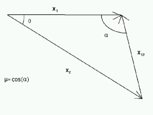
Figure 1: This shows the various distances and angles involved in calculating ${w}(\nu_{1},\nu_{2},\theta)$, where $\nu_{1}$ can be converted to $x_{1}$ using equation (1).

The form of the angular correlation is further simplified if we restrict $\theta$ to be very small. Under this assumption $\boldsymbol{n}_{1}\simeq\boldsymbol{n}_{2}$, and we use $\boldsymbol{n}$ to denote the common line of sight. We also use $\mu=\boldsymbol{n}\cdot(\boldsymbol{x}_{1}-\boldsymbol{x}_{2})/x_{12}$ for the cosine of the angle between the line of sight $\boldsymbol{n}$ and the vector $\boldsymbol{x}_{1}-\boldsymbol{x}_{2}$ joining the two points between which we are measuring the correlation. The relation between the different distances and angles is shown in figure 1, and we have $x_{12}=\sqrt{x_{1}^{2}+x_{2}^{2}-2x_{1}x_{2}\cos(\theta)}$ and $\mu=(x_{1}-x_{2}\cos(\theta))/x_{12}$. Using these we finally obtain the following expression for the two point correlation of the temperature

$${w}(\nu_{1},\nu_{2},\theta) = \bar{T}_{1}\bar{T}_{2}D_{1}D_{2}b_{2}b_{2}\left\{\left[(1+\beta_{1}\mu^{2})(1+\beta_{2}\mu^{2})\right]\tilde{\xi}(x_{12})\right.$$ (22)

$$+ \left.\left[(\frac{1}{3}-\mu^{2})(\beta_{1}+\beta_{2})+(\frac{1}{2}-3\mu^{2}+\frac{5}{2}\mu^{4})\beta_{1}\beta_{2}\right]\tilde{\xi_{2}}(x_{12})\right.$$

$$- \left.\left[\frac{3}{10}+3\mu^{2}-\frac{7}{2}\mu^{4}\right]\tilde{\xi_{4}}(x_{12})\right\}$$

3 Predictions for different models.

The density of HI ($\Omega_{\rm HI}$) in DLAs has been determined reasonably well for $0\leq z\leq 3$ from absorption studies (Lanzetta, Wolfe, & Turnshek 1995) and they find that the observed evolution of $\Omega_{\rm HI}$ is well approximated by $\Omega_{\rm HI}(z)=\Omega_{\rm HI0}\exp(\alpha\,z)$ with $\Omega_{\rm HI0}=0.18\pm 0.04\times 10^{-3}h^{-1}$ and $\alpha=0.60\pm 0.15$ for $q_{0}=0$, and $\Omega_{\rm HI0}=0.19\pm 0.04\times 10^{-3}h^{-1}$ and $\alpha=0.83\pm 0.15$ for $q_{0}=0.5$, We have used this to calculate the isotropic part of the background brightness temperature due to the redshifted HI emission (equation 17). We have considered two spatially flat FRW cosmological models with parameters (I) $\Omega_{m0}=1.0$ and $\lambda_{0}=0$, and (II) $\Omega_{m0}=0.3$ and $\lambda_{0}=0.7$, with $h=0.5$ in both cases. It should be pointed out that the fits given Lanzetta et al. (1995) are not valid for the model with a cosmological constant, and we use the $q_{0}=0$ fit in this case.

Figure 2 shows the brightness temperature as a function of frequency for both the cases.

We find that the temperature increases rapidly as we go to lower frequencies (higher $z$) and it is around $1\,{\rm mK}$ at $\nu\sim 330{\rm MHz}$ which corresponds to $z\sim 3$. The increase in the temperature is a direct consequence of the increase of HI density with increasing redshift. The HI density is not very well determined at $z>3$ and there is evidence that $\Omega_{\rm HI}$ falls off at higher redshifts (Storrie–Lombardi et al. 1996).

We next consider ${w}(\nu_{1},\nu_{2},\theta)$ the cross-correlation in the temperature fluctuation at different frequencies which we have calculated for the two cases discussed above. We have calculated the dark-matter two point correlation function (equation 20) using the analytic fitting form for the CDM power spectrum given by Efstathiou, Bond and White (1992). For case (I) we use a value of the shape parameter $\Gamma=0.25$ and for (II) we use $\Gamma=0.14$. The power spectra are normalized using the results of Bunn and White (1996) based on the 4-year COBE data. It should be noted that he redshift evolution of the matter correlation function and $f(\Omega_{m})$ are quite different in the two cases that we have considered. The predictions for ${w}(\nu_{1},\nu_{2},\theta)$ are shown in figures 3 and 4. We have assumed that the HI faithfully traces the matter distribution and set $b(\nu)=1$ throughout.

In our analysis we have kept $\nu_{1}$ fixed at $320{\rm MHz}$ and let $\nu_{2}$ vary over a band of $16{\rm MHz}$ centered around $\nu_{1}$, while $\theta$ takes values upto $2^{\circ}$. In order to measure ${w}(\nu_{1},\nu_{2},\theta)$ over this range we would need radio images of the background temperature fluctuation in a $2^{\circ}\times 2^{\circ}$ field at different frequencies in a $16{\rm MHz}$ band centered around $320{\rm MHz}$ and ${w}(\nu_{1},\nu_{2},\theta)$ could be estimated using

$${w}(\nu_{1},\nu_{2},\theta)=\langle\Delta T_{\nu_{1}}(\boldsymbol{n}_{1})\Delta T_{\nu_{2}}(\boldsymbol{n}_{2})\rangle$$ (23)

where $\Delta T_{\nu_{1}}(\boldsymbol{n}_{1})$ refers to the temperature fluctuation along the direction $\boldsymbol{n}_{1}$ in the image made at frequency $\nu_{1}$, and the angular brackets denote average over all pairs of directions $\boldsymbol{n}_{1}$ and $\boldsymbol{n}_{2}$ which are separated by an angle $\theta$. The central frequency, bandwidth and angular range have been chosen keeping in mind the Giant Meter wave Radio Telescope (GMRT, Swarup et al.  1991) which has recently become operational. The frequency intervals and angular separation can be converted to a corresponding comoving length-scale and in case (I) $1{\rm MHz}=8.9{\rm Mpc}$ and $1^{{}^{\prime}}=1.8{\rm Mpc}$, while in case (II) $1{\rm MHz}=16.0{\rm Mpc}$ and $1^{{}^{\prime}}=2.7{\rm Mpc}$. The linear theory of density perturbations which we have used here can be applied at scales $\geq 10{\rm Mpc}$, which covers most of the region shown in the figures.

We find that ${w}(\nu_{1},\nu_{2},\theta)$ is between $10^{-7}{\rm K}^{2}$ to $10^{-8}{\rm K}^{2}$ when the comoving-distance corresponding to the separation in frequencies and direction is less between $10{\rm Mpc}$ and $40{\rm Mpc}$ beyond which it falls off. The cross-correlation between the temperature fluctuations is expected to be larger at small scales where the linear theory of density perturbations will not be valid and we have not considered these scales here. The temperature fluctuations are anti-correlated when the separation in frequencies exceeds the angular separation. This occurs because of the effect of the peculiar velocity which produces a “distortion” very similar to the effect it has on the two-point correlation function in redshift surveys.

4 Observational prospects

In this section we discuss the prospects of actually observing the background radiation from the HI in damped Lyman-$\alpha$ clouds. Our discussion is restricted to observations at around $320\,{\rm MHz}$ largely because we have reliable estimates of the HI content at $z\leq 3$ and there are indications that $z\simeq 3$ might be the redshift where the HI content of the universe is maximum (Storrie–Lombardi et al. 1996). Another reason for our choice of this frequency range is that the GMRT (Swarup et al.  1991) which is already functioning at these frequencies is expected to have an angular resolution of $10^{{}^{\prime\prime}}$ and reach noise levels of $100{\rm\mu K}$ in around 10 hrs of integration. The angular resolution and sensitivity of the GMRT will be sufficient for detecting both the isotropic component as well as the correlations in the component of the background radiation arising from the HI at $z\simeq 3$ (Figures 2, 3 and 4) provided we can distinguish this component from the contribution due to other sources.

4.1 Galactic and extra-galactic foregrounds

Any observations at low frequencies will have a very large contribution from the synchrotron radiation from our own galaxy. Observations at $408\,\rm MHz$ (Haslam et al. 1982) with resolution $1^{\circ}\hbox{x}1^{\circ}$ indicate a minimum temperature of $\simeq 10\,\rm K$ at $408\,{\rm MH}z$. Using $T\propto\nu^{-2.7}$ as indicated by the spectral index of galactic synchrotron radiation, the temperature at $\nu\simeq 320\,\rm MHz$ is $\simeq 20\,\rm K$. Comparing this number with the expected background from redshifted HI radiation (Figure 2) the galactic foreground is seen to be several orders above the expected signal. Another quantity of interest to us is the fluctuations in the galactic radiation at angles $\lower 2.15277pt\hbox{$\;\buildrel<\over{\sim}\;$}1^{\circ}$. However as the resolution of Haslam maps is $\simeq 1^{\circ}$ it cannot be used to make any predictions about the fluctuations at the angular scales of interest.

Another source of contamination is the continuum radiation from unresolved extragalactic sources (the resolved ones will be removed from the image before analysis) and we use results from the recent FIRST survey (for details see White et al. 1997 and references therein) to estimate this. Tegmark & Estathiou (1995) provide an analytic fit for the number of sources per unit flux $\phi[{\rm mJy}]$ per steradian in this survey, and at flux levels $\phi\ll 100{\rm mJy}$ this can be approximated by

$${dn\over d\phi}={5.24\times 10^{5}\over{\rm mJy\,sr}}\left({\phi\over 0.75{\rm mJy}}\right)^{-1.65}\,.$$ (24)

We use this to estimate the total contribution from sources fainter than $100\,\mu{\rm Jy}$, and converting this to brightness temperature we find that the continuum emission from unresolved radio sources is expected to produce a background radiation with brightness temperature $\sim.1\rm K$ at $1.5\,{\rm Ghz}$. For the purposes of estimating an order-of-magnitude we assume this value to be representative of what we expect at $\sim 320\,\rm MHz$.

The two-point correlation function of the sources detected by FIRST has been estimated (Cress et al. 1996): $w(\theta)\simeq 0.18\theta^{-1.1}$, with $\theta$ in $\rm arcminutes$. Little is known about the correlations expected in the fluctuations in the contribution to the background radiation from unresolved radio sources.

It is clear from the foregoing discussion that both galactic and extragalactic continuum signals are likely to be so high that they would totally swamp the signal which we want to detect and therefore it is not possible to directly detect the radiation from HI unless we find some method for removing the foregrounds.

At present the most promising strategy is to use the proposed observations themselves to determine the foreground and remove this from the data, and we next discuss a possible method for doing this.

4.2 Removing foregrounds

We consider the GMRT band centered at $325\,\rm MHz$ for our discussion in this section. The total bandwidth of $16\,\rm MHz$ is divided in 128 channels each with $\Delta\nu=1.25\,\rm kHz$, and the signal in any frequency channel is expected to be dominated by the foregrounds.

Here we briefly review the standard method of continuum subtraction which is generally used in spectral line detections and then discuss how this method can be used for the analysis proposed here. The reader is referred to Subrahmanyam and Anantharamaiah (1990) and references therein for examples of how this method is applied in searches for HI emission from protoclusters.

We represent the observed signal $y_{i}(\boldsymbol{n})$ in the $i$ th frequency channel in the direction $\boldsymbol{n}$ as:

$$y_{i}(\boldsymbol{n})=x_{i}(\boldsymbol{n})+f_{i}(\boldsymbol{n})+N_{i}$$ (25)

where $x_{i}(\boldsymbol{n})$ and $f_{i}(\boldsymbol{n})$ are the contribution to the output signal from the HI and the foregrounds respectively, and $N_{i}$ is the receiver noise.

We should at this stage remind ourselves that foregrounds are sources which are emitting continuum radiation—the primary such source being the synchrotron radiation from our own galaxy. We also have the contribution from unresolved extragalactic radio sources which, as we have seen above, is a smaller contribution. The sum total of these along any line of sight is expected to be a smooth function of the frequency. On the contrary the contribution from the HI will come from individual damped Lyman $\alpha$ clouds along the line of sight with a velocity width $\simeq 200\,\rm km\,sec^{-1}$ (Prochaska & Wolfe 1998) and this will correspond to lines of width:

$$\Delta\nu\sim\frac{\Delta V}{c}\nu\simeq 0.2{\rm MHz}.$$ (26)

Although the total number of damped Lyman-$\alpha$ clouds in a $1^{\circ}\times 1^{\circ}\times\,16\,{\rm MHz}$ field is expected to be quite large $(\simeq 3\times 10^{4})$ we expect to have only one damped Lyman-$\alpha$ cloud along a single $20^{{}^{\prime\prime}}\times 20^{{}^{\prime\prime}}\times 16\,{\rm MHz}$ synthesized GMRT beam. The probability of two damped Lyman-$\alpha$ clouds occurring right next to each other in the same synthesized beam and causing confusion is quite small, and hence the signal we are looking for will come in the form of lines of width $\sim 0.2{\rm MHz}$ which we will not be able to detect as the individual lines will be swamped by both the foreground as well as the noise. What we can do is to fit the smooth component of the signal $y_{i}(\boldsymbol{n})$ by a function $F_{i}(\boldsymbol{n})$ and subtract this from the output signal to remove the effect of the foregrounds

$$S_{i}(\boldsymbol{n})=y_{i}(\boldsymbol{n})-F_{i}(\boldsymbol{n})=x_{i}(\boldsymbol{n})+N_{i}(\boldsymbol{n})+E_{i}(\boldsymbol{n})$$ (27)

where we call $S_{i}(\boldsymbol{n})$ the reduced signal and $E_{i}(\boldsymbol{n})$ is the possible error in the fitting procedure. If our foreground subtraction works correctly, the reduced signal should have contributions from only the HI signal and the noise.

We first determine the mean reduced signal

$$\bar{S}_{i}=\left\langle S_{i}(\boldsymbol{n})\right\rangle=\left\langle x_{i}(\boldsymbol{n})\right\rangle+\left\langle N_{i}(\boldsymbol{n})\right\rangle+\left\langle E_{i}(\boldsymbol{n})\right\rangle$$ (28)

where the angular brackets denote average over all lines of sight. If the errors in the foreground subtraction can be made smaller than the signal i.e. $\langle E_{i}(\boldsymbol{n})\rangle\,<\,\langle x_{i}(\boldsymbol{n})\rangle$ then this will give an estimate of the background brightness temperature due to the HI emission i.e. $\bar{T}(\nu)=\bar{S}_{i}$ where the index $i$ refers to the channel with central frequency $\nu$.

We next consider the quantity

$$\Delta S_{i}(\boldsymbol{n})=S_{i}(\boldsymbol{n})-\bar{S}_{i}$$ (29)

which gives the fluctuation in the brightness temperature. We can use this to estimate the cross-correlation in the fluctuations at different frequencies

$${w}(\nu_{1},\nu_{2},\theta)=\langle\Delta S_{i}(\boldsymbol{n})\Delta S_{j}({\bf m})\rangle$$ (30)

where $i$ and $j$ are the channel with frequency $\nu_{1}$ and $\nu_{2}$ respectively, and $\boldsymbol{n}$ and ${\bf m}$ are two lines of sight separated by an angle $\theta$ and the angular brackets denote average over all such pairs of lines of sight.

5 Summary and Conclusions

We have investigated the contribution from the HI in unresolved damped Lyman-$\alpha$ clouds at high redshifts to the background radiation at low frequency radio waves (meter waves). The isotropic part of this radiation depends on the density of HI and the background cosmological model, while the fluctuations in this component of the background radiation have an added dependence on the fluctuations in the distribution of the damped Lyman-$\alpha$ clouds and their peculiar velocities.

We have used estimates of the HI density available from absorption studies to calculate the brightness temperature of this radiation. We find that this has a value $\sim 1\,{\rm mK}$ at $320\,{\rm MHz}$ which corresponds to $z\sim 3$. The distribution of damped Lyman-$\alpha$ clouds is assumed to trace the underlying dark matter distribution which also determines the peculiar velocities. Using this and the linear theory of density perturbations, we have calculated the relation between the fluctuation in this component of the background radiation and the density perturbations at high $z$. Observations of the cross-correlations of the fluctuations at different sight lines across images produced at different frequencies holds the possibility of allowing us to probe the two point correlation function (or power spectrum) at high redshifts. We have calculated the expected cross-correlations for two currently acceptable CDM models and find it to be in the range $10^{-7}{\rm K^{2}}$ to $10^{-8}{\rm K^{2}}$ at $\nu\sim 320{\rm MHz}$ for separations in sight lines and frequencies such that the corresponding spatial separation is in the range $10\,{\rm Mpc}$ and $40\,{\rm Mpc}$. The cross-correlations are expected to be larger at smaller scales where the linear theory cannot be applied. Our results show that both the isotropic background (Figure 2) and its fluctuations (Figure 3 and  4) can be detected by GMRT which is the largest telescope operating at meter waves at present, provided this signal can be distinguished from other sources which contribute to the low frequency background radiation.

The biggest obstacles in detecting the HI contribution are the galactic and extra-galactic foregrounds, both of which are many orders larger than the signal we want to detect. The fact that both those sources of contamination emit continuum radiation while the HI contribution is from individual damped Lyman-$\alpha$ clouds each of which emits a spectral line with a relatively small velocity width keeps alive the possibility of being able to distinguish this signal from the contamination. We have, in this paper, considered one possible approach which might allow us to model and subtract the foreground along any line of sight. More work is needed in this direction and work is currently underway in investigating other viable possibilities for foreground removal.

Figure 2: This shows the isotropic part of the brightness temperature at different frequencies. The solid line shows model (I) and the dashed line model (II) of section 3.

Figure 3: For $\Omega_{m0}=1,h=0.5$, (a) shows ${w}(\nu_{1},\nu_{2},\theta)$ in ${\rm K}^{2}$ vs. $\theta$ with $\nu_{1}=320{\rm MHz}$ and curves (1),(2) and (3) corresponding to $\nu_{2}=320{\rm MHz}$, $322{\rm MHz}$ and $324{\rm MHz}$ respectively; (b) shows contours of equal ${w}(\nu_{1},\nu_{2},\theta)$ at logarithmic intervals of ${w}$ with $\nu_{1}=320{\rm MHz}$. Here $1{\rm MHz}=8.9{\rm Mpc}$ and $1^{{}^{\prime}}=1.8{\rm Mpc}$. The dashed lines show negative values of $w$.

Figure 4: For $\Omega_{m0}=0.3,\lambda_{0}=0.7,h=0.5$, (a) shows ${w}(\nu_{1},\nu_{2},\theta)$ in ${\rm K}^{2}$ vs. $\theta$ with $\nu_{1}=320{\rm MHz}$ and curves (1),(2) and (3) corresponding to $\nu_{2}=320{\rm MHz}$, $322{\rm MHz}$ and $324{\rm MHz}$ respectively; (b) shows contours of equal ${w}(\nu_{1},\nu_{2},\theta)$ at logarithmic intervals of ${w}$ with $\nu_{1}=320{\rm MHz}$. Here $1{\rm MHz}=16.0{\rm Mpc}$ and $1^{{}^{\prime}}=2.7{\rm Mpc}$. The dashed lines show negative values of $w$.

References

- Bagla (1999) Bagla, J. S. 1999, ASP Conf. Ser. 156: Highly Redshifted Radio Lines, 9
- (2) Bagla J.S., Nath B. and Padmanabhan T. 1997, MNRAS, 289, 671
- (3) Barcons, X., Carrera, F. J., Ceballos, M. T., & Mateous, S. 2000, astro-ph/0001191
- (4) Barcons, X., Fabian, A. C., & Carrera, F. J. 1998, MNRAS, 293, 60
- (5) Bond, J. R. 1996, Observations of Large-Scale Structure in the universe , Ed. R. Schaeffer et al. , Les Houches, Elsevier Science
- (6) Bardeen, J. M., Bond, J. R., Kaiser, N., & Szalay, A. S. 1986, ApJ, 304, 1
- (7) Bunn E. F. & White M. 1996, astro-ph/9607060
- (8) Cress, C. M., et al. 1996, ApJ, 473, 7
- (9) Gorjian, V.. Wright E. L. & Chary R.R., 1999, ApJ, in Press, astro-ph/9909428
- (10) Haslam, C. G. T., Stoffel, H. , Salter, C. J. & Wilson, W. E. 1982, ApJS, 47, 1
- (11) Kashlinsky, A., Mather, J. C., & Odenwald, S. 1999, astro-ph/9908304
- (12) Kashlinsky, A., Mather, J. C., & Odenwald, S. 1997, astro-ph/9701216
- Katz, Hernquist and Weinberg (1999) Katz, N., Hernquist, L. and Weinberg, D. H. 1999, ASP Conf. Ser. 156: Highly Redshifted Radio Lines, 1
- (14) Kumar A., Padmanabhan T. and Subramanian K. 1995, MNRAS, 272, 544
- (15) Lahav O., Lilje P. B., Primack J. R. and Rees M., 1991, MNRAS, 251, 128
- (16) Lanzetta, K. M., Wolfe, A. M., Turnshek, D. A. 1995, ApJ, 430, 435
- (17) Peacock, J. A. 1999, Cosmological Physics , Cambridge, Cambridge University Press
- (18) Peebles, P. J. E. Principles of Physical Cosmology , Princeton, Princeton University Press
- (19) Peebles, P. J. E. 1980, The Large-Scale Structure of the Universe , Princeton, Princeton University Press
- (20) Prochaska, J. X. & Wolfe, A. M. 1998, ApJ, 507, 113
- Shaver, Windhorst, Madau and de Bruyn (1999) Shaver, P. A., Windhorst, R. A., Madau, P. and de Bruyn, A. G. 1999, A&A, 345, 380
- (22) Shectman, S. A. 1974, ApJ, 188, 233
- (23) Storrie–Lombardi, L.J., McMahon, R.G., Irwin, M.J. 1996, MNRAS, 283, L79
- (24) Subramanian, K. and Padmanabhan, T. 1993, MNRAS, 265, 101
- (25) Subrahmanyam. R. & Anantharamaiah, K. R. JAA, 1990, 11, 221:
- (26) Sunyaev, R. A. & Zel’dovich, Ya. B. 1975, MNRAS, 171, 375
- (27) Swarup, G., Ananthakrishan, S., Kapahi, V. K., Rao, A. P., Subrahmanya, C. R., & Kulkarni, V. K. 1991, Curr. Sci., 60, 95
- (28) Tegmark, M, & Efstathiou, G. 1996, MNRAS, 281, 1297
- Tozzi, Madau, Meiksin and Rees (2000) Tozzi, P., Madau, P., Meiksin, A. and Rees, M. J. 2000, ApJ, 528, 597
- (30) White, R. L., Becker, R. H., Gregg, M. D. & Helfand, D. J. 1997, ApJ, 475, 479
- (31) Efstathiou, G., Bond, J. R. & White, S. D. M. 1992, MNRAS, 250, 1p