Ekman layers and the damping of inertial r-modes in a spherical shell: application to neutron stars

Abstract

Recently, eigenmodes of rotating fluids, namely inertial modes, have received much attention in relation to their destabilization when coupled to gravitational radiation within neutron stars. However, these modes have been known for a long time by fluid dynamicists. We give a short account of their history and review our present understanding of their properties. Considering the case of a spherical container, we then give the exact solution of the boundary (Ekman) layer flow associated with inertial r-modes and show that previous estimations all underestimated the dissipation by these layers. We also show that the presence of an inner core has little influence on this dissipation. As a conclusion, we compute the window of instability in the temperature/rotation plane for a crusted neutron star when it is modeled by an incompressible fluid.

1 Introduction

Recently much work has been devoted to the study of the rotational instability of neutron stars resulting from a coupling between gravitational radiation and the so-called “r-modes” of a rotating star Andersson (1998); Friedman and Morsink (1998); Lindblom et al. (1998); Kokkotas and Stergioulas (1999). Such an instability may indeed play a key role in the distribution of rotation periods of neutron stars as well as it may be an important source of gravitational radiation.

In this paper, we shall first clarify a point of history concerning “r-modes” which are in fact a special class of inertial modes; we shall then review their singular properties which have been clarified only very recently in Rieutord and Valdettaro (1997), Rieutord et al. (2000a) and Rieutord et al. (2000b). The last section will present the analytical derivation of the damping rate of inertial r-modes in a neutron star with a crust and/or a core through the boundary layer analysis within the framework of newtonian theory. We conclude on the stability of crusted neutron stars when modeled by an incompressible viscous fluid in a rotating sphere.

2 A short point of history

The very first work on rotating fluids oscillations which are presently known as inertial modes dates back to Thomson (1880) who analysed the case of a fluid contained in a cylinder. However, another impetus to the study of these oscillations was given soon after by Poincaré’s (1885) work on the stability of rotating self-gravitating masses, a work applied to MacLaurin spheroids by Bryan (1889) and later continued by Cartan (1922) who christened the equation of inertial modes as “Poincaré equation”. In these studies, however, the effect of rotation is combined to the one of gravity through (for an incompressible fluid) surface gravity waves. In fact, except for the work of Thomson, investigations on the oscillations specific of rotating fluids seem to have started with the work of Bjerknes et al. (1933) where they are called “elastoid-inertial oscillations” since conservation of angular momentum makes axis-centered rings of fluid behave elastically; but see Fultz (1959) or Aldridge (1967) for an account on this part of history. In the sixties, much work has been devoted to these oscillations, mainly by Greenspan who introduced the terminology of “inertial oscillations”. The presently used denomination “inertial modes” has been “officially” given by Greenspan’s book (Greenspan, 1969).

However, inertial modes are somewhat too general for applications in some specific domains like atmospheric sciences. In this field indeed motions are essentially two dimensional and inertial modes may be simplified into the well-known Rossby (or planetary) waves.

The introduction of r-modes by Papaloizou and Pringle (1978) was quite unfortunate since they associated eigenmodes of rotating fluids with a very special class of inertial modes, namely purely toroidal inertial modes. This lead following authors to introduce weird names such as “hybrid modes” or “generalized r-modes” (Lockitch and Friedman, 1999) for describing the general class of inertial modes. We therefore encourage authors to use, as fluid dynamicists, inertial modes unless they discuss the very specific r-modes.

3 The present theory of inertial modes

Inertial modes are a class of modes of oscillation of rotating fluids which owe their existence to the Coriolis force. This force of inertia has indeed a restoring action on perturbations of rotating fluids since it insures the global conservation of angular momentum. These modes have many properties similar to those of gravity modes of stably stratified fluids (Rieutord and Noui, 1999).

The dynamics of inertial modes may be appreciated when all other effects are suppressed: no compressibility, no magnetic fields, no gravity, etc… only an incompressible inviscid rotating (like a solid body) fluid. In this case, perturbations of velocity $\delta{\bf v}$ and pressure $\delta P$ obey

$$\frac{\partial\delta{\bf v}}{\partial t}+2{\bf\Omega}\times\delta{\bf v}=-{\rm NewA}\delta P,\qquad{\rm NewA}\cdot\delta{\bf v}=0$$ (1)

where ${\bf\Omega}$ is the angular velocity of the fluid. Concentrating on time-periodic oscillations and choosing $(2\Omega)^{-1}$ as the time scale, (1) can be written

$$i\omega{\bf u}+{\bf e}_{z}\times{\bf u}=-{\rm NewA}p,\qquad{\rm NewA}\cdot{\bf u}=0$$ (2)

with non-dimensional variables; $\omega$ is the non-dimensional (real) frequency. When the velocity ${\bf u}$ is eliminated in favor of the pressure perturbation $p$, one is left with

$$\Delta p-\frac{1}{\omega^{2}}\frac{\partial^{2}p}{\partial z^{2}}=0$$ (3)

which is known as Poincaré equation since Cartan (1922). This equation is remarkable in the fact that it is hyperbolic spatially since $|\omega|\leq 1$ (Greenspan, 1969). As the solution of (3) must meet boundary conditions, namely ${\bf u}\cdot{\bf n}=0$, we see that inertial modes are solutions of an ill-posed boundary value problem. This property means that, in general, inertial modes are singular; in other words they cannot exist physically if the fluid is strictly inviscid. These properties are detailed in Rieutord and Valdettaro (1997) and Rieutord et al. (2000a); to make a long story short, one may summarize the situation as follows.

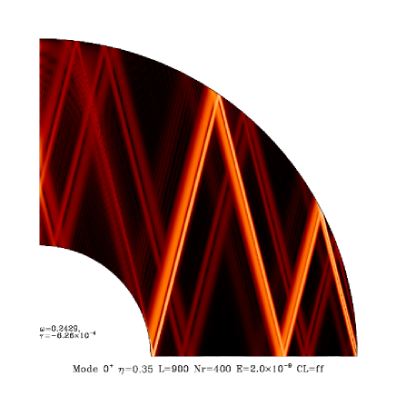
Figure 1: The kinetic energy distribution in a meridional plane of an inertial mode in a spherical shell associated with an equatorial attractor. A co-existing polar attractor is also slightly excited. The mode is axisymmetric with equatorial symmetry. Stress-free boundary conditions have been used on both shells; this solution was computed with an Ekman number of 2 10^-9 and required 1300 spherical harmonics and 450 radial grid points (Gauss-Lobatto). The ratio of the inner radius to the outer radius is $\eta=0.35$. $\omega=0.2429$ and the damping rate $\tau=-6.26\times 10^{-4}$ are given in dimensionless units as equation (2).

Let us first recall that in hyperbolic systems, energy propagates along the characteristics of the equation. For the Poincaré problem, these are straight lines in a meridional plane. A way to approach the solutions of this difficult problem is to examine the propagation of characteristics as they reflect on the boundaries. They define trajectories which depend strongly on the container. Let us therefore concentrate on the case of a spherical shell as a container; this configuration is relevant for neutron stars with a central core due to some phase transition of the nuclear matter (see Haensel, 1996). In this case, it may be shown that characteristic trajectories generically converge towards attractors which are periodic orbits. It may be shown (Rieutord et al., 2000a) that in this case, the associated solutions are singular, namely the velocity field is not square-integrable. However, inertial r-modes are still solutions of the problem since they meet the boundary conditions ($u_{r}=0$); in fact they are the only regular (square-integrable) solutions of the Poincaré problem in a spherical shell. In a more mathematical way, we may say that the spectrum of eigenvalues of the Poincaré problem in a spherical shell is empty except for the inertial r-modes. In this sense, these modes are quite exceptional. This situation occurs because there exists no system of coordinate in which the dependent variables of the Poincaré equation can be separated. This is a consequence of the conflict between the symmetry of the Coriolis force (cylindrical) and the geometry of the boundaries. Thus, when this constraint is relaxed, like in the case of a cylindrical container, regular solutions exist and a dense spectrum of eigenvalues appears in the allowed frequency range, namely $[0,2\Omega]$. In the case the container is a full sphere, attractors also disappear and eigenmodes exist; they are also related to a dense spectrum of eigenfrequencies. In this case, Poincaré equation is exactly solvable (Greenspan, 1969).

However, real fluids have viscosity ($\nu$) and equation (2) should be transformed into

$$\lambda{\bf u}+{\bf e}_{z}\times{\bf u}=-{\rm NewA}p+E\Delta{\bf u},\qquad{\rm NewA}\cdot{\bf u}=0$$ (4)

where $\lambda$ is the complex eigenvalue and $E=\nu/2\Omega R^{2}$ is the Ekman number ($R$ is the outer radius of the shell).

Using no-slip (${\bf u}={\bf 0}$) or stress-free boundary conditions, (4) yields a well-posed problem. Yet, the singularities of the associated inviscid solutions show up through the existence of shear layers. As shown by fig. 1, the shape of inertial modes is deeply influenced by the underlying singularity of the inviscid solution. We have shown (Rieutord et al., 2000a) that these shear layers are in fact nested layers with different scales for their inner part scales as $E^{1/3}$ and their outer part seems to scale with $E^{1/4}$. Because of these internal shear layers, these modes are strongly damped.

We therefore see that according to whether a neutron star has a central core or not, the damping of inertial modes will be extremely different. If there is a central core, the only regular modes are the inertial r-modes which will be by far the least damped; if there isn’t any core then a dense spectrum exists (Greenspan, 1969; Lockitch and Friedman, 1999) but inertial r-modes remain the most unstable because of their simple structure.

4 Damping of toroidal inertial modes in a sphere or a shell

We shall now give the expression of the viscous damping of inertial r-modes when one of the boundary is solid therefore when the dissipation is due to Ekman boundary layers; we shall thus complete the works of Bildsten and Ushomirsky (2000) and Andersson et al. (2000) by giving the rigorous estimate of the damping rate; the method which we use here has been outlined in Greenspan (1969).

The damping rate is given by:

$$\gamma=\Re e(\lambda)=-E\frac{\int({\rm NewA}:{\bf u})^{2}dV}{\int{\bf u}^{2}dV}$$ (5)

where $({\rm NewA}:{\bf u})^{2}$ stands for the squared rate-of-strain tensor (see below). The velocity field of r-modes is

$$\overline{u}_{\theta}=Ar^{m}(\sin\theta)^{m-1}\sin(m\phi+\omega_{m}t)$$

$$\overline{u}_{\varphi}=Ar^{m}(\sin\theta)^{m-1}\cos\theta\cos(m\phi+\omega_{m}t)$$

The kinetic energy integral may be evaluated explicitly

$$\int{\bf u}^{2}dV=\pi A^{2}\left(1-\eta^{2m+3}\right)\frac{2^{m+1}(m+1)!}{m(2m+3)!!}$$ (6)

where $\eta$ is the ratio of the radius of the inner boundary to the one of the outer boundary.

The dissipation integral need more work if one of the boundary is no-slip. In this case, dissipation is essentially coming from the Ekman layers and thus we need to derive the flow in these layers. The method has been given by Greenspan from whom we know that the boundary layer correction $\tilde{u}$, is related to the interior solution $\overline{u}$ by

$$\tilde{u}_{\theta}+i\tilde{u}_{\varphi}=-(\overline{u}_{\theta}+i\overline{u}_{\varphi})_{r=r_{b}}e^{-\zeta\sqrt{i\cos\theta\pm i\omega}}$$ (7)

where $\zeta$ is the radial scaled variable $(r-r_{b})/\sqrt{E}$ with $r_{b}$ as the radius of the boundary (1 or $\eta$). The complete solution is then ${\bf u}=\tilde{u}+\overline{u}$; setting $\beta=\omega t+m\varphi$ we have

$$\overline{u}_{\theta}+i\overline{u}_{\varphi}=\frac{Ar^{m}(\sin\theta)^{m-1}}{2i}\hskip 56.9055pt$$

$$\qquad\times\left\{(1-\cos\theta)e^{i\beta}-(1+\cos\theta)e^{-i\beta}\right\}$$

from which it follows that

$$\tilde{u}_{\theta}+i\tilde{u}_{\varphi}=\frac{Ar_{b}^{m}(\sin\theta)^{m-1}}{2i}\left\{(1+\cos\theta)e^{-i\beta-\zeta\sqrt{i\cos\theta-i\omega}}\right.$$

$$-\left.(1-\cos\theta)e^{i\beta-\zeta\sqrt{i\cos\theta+i\omega}}\right\}$$

Now we need the expression of the square of the rate-of-strain tensor $s_{ij}=\partial_{i}v_{j}+\partial_{j}v_{i}$ in spherical coordinates, viz

$$({\rm NewA}:{\bf u})^{2}=s_{rr}^{2}+s_{\theta\theta}^{2}+s_{\phi\phi}^{2}+2(s_{r\theta}^{2}+s_{r\phi}^{2}+s_{\theta\phi}^{2})$$

Since the radial derivatives dominate, this expression reduces to the contribution of the tangential stresses. Using the scaled coordinate, $\zeta=|r-r_{b}|/\sqrt{E}$, we have

$$({\rm NewA}:{\bf u})^{2}=\frac{2}{E}\left\{\left(\frac{\partial u_{\theta}}{\partial\zeta}\right)^{2}+\left(\frac{\partial u_{\varphi}}{\partial\zeta}\right)^{2}\right\}_{r=r_{b}}$$

We now set $p=\cos\theta-\omega$ and $q=\cos\theta+\omega$. We thus get

$$({\rm NewA}:{\bf u})^{2}=\frac{A^{2}r_{b}^{2m}(\sin\theta)^{2m-2}}{2E}\left\{(1+\cos\theta)^{2}|p|e^{-\zeta\sqrt{2|p|}}\right.$$

$$+(1-\cos\theta)^{2}|q|e^{-\zeta\sqrt{2|q|}}$$

$$\left.-2\sin^{2}\theta\sqrt{pq}\;\Re e\left(e^{2i\beta-\zeta(\sqrt{iq}+\sqrt{-ip})}\right)\right\}$$

Integrating over the $\varphi$-variable yields

$$\int_{0}^{2\pi}({\rm NewA}:{\bf u})^{2}d\varphi=\frac{\pi A^{2}r_{b}^{2m}(\sin\theta)^{2m-2}}{E}\hskip 56.9055pt$$

$$\times\left\{(1+\cos\theta)^{2}|p|e^{-\zeta\sqrt{2|p|}}+(1-\cos\theta)^{2}|q|e^{-\zeta\sqrt{2|q|}}\right\}$$ (8)

We now integrate over the radial variable:

$$\int_{\eta}^{1}\int_{0}^{2\pi}({\rm NewA}:{\bf u})^{2}d\varphi\;r^{2}dr=\hskip 56.9055pt$$

$$\frac{\pi A^{2}(\sin\theta)^{2m-2}}{E}\int_{\eta}^{1}r^{2m+2}f(\zeta)dr$$

with $f(\zeta)=(1+\cos\theta)^{2}|p|e^{-\zeta\sqrt{2|p|}}+(1-\cos\theta)^{2}|q|e^{-\zeta\sqrt{2|q|}}$; since $r=\eta+\sqrt{E}\zeta$ or $r=1-\sqrt{E}\zeta$ according to which side of the integral is chosen, it turns out that

$$\int_{\eta}^{1}\!\int_{0}^{2\pi}({\rm NewA}:{\bf u})^{2}d\varphi\;r^{2}dr$$

$$= K\int_{0}^{\infty}\left[(1+\cos\theta)^{2}|p|e^{-\zeta\sqrt{2|p|}}\right.$$

$$+\left.(1-\cos\theta)^{2}|q|e^{-\zeta\sqrt{2|q|}}\right]d\zeta$$

$$= \frac{K}{\sqrt{2}}\left[(1+\cos\theta)^{2}\sqrt{|\cos\theta-\omega|}\right.$$

$$+\left.(1-\cos\theta)^{2}\sqrt{|\cos\theta+\omega|}\right]$$

with $K=\pi A^{2}(\sin\theta)^{2m-2}P(\eta)/\sqrt{E}$, where $P(\eta)$ is a function depending on the boundary conditions (see table 1). Finally integrating over $\theta$, we find

$$\int({\rm NewA}:{\bf u})^{2}dV=\frac{2\pi A^{2}P(\eta)}{\sqrt{2E}}{\cal I}_{m}$$ (9)

with

$${\cal I}_{m}=\int_{0}^{\pi}(1+\cos\theta)^{2}\sqrt{|\cos\theta-\omega|}\sin^{2m-1}\theta d\theta$$ (10)

Finally grouping (6) and (9), we find the damping rate

$$\gamma=-\frac{m(2m+3)!!}{2^{m+3/2}(m+1)!}Q(\eta){\cal I}_{m}\sqrt{E}$$ (11)

where $Q(\eta)=P(\eta)/\left(1-\eta^{2m+3}\right)$.

Outer B.C. no-slip stress-free Inner B.C. no-slip $1+\eta^{2m+2}$ $\eta^{2m+2}$ stress-free 1 No Ekman layer

Table 1: Expression of the $P(\eta)$ function according to boundary conditions.

For the cases $m=1$ and $m=2$ we evaluated the expression of ${\cal I}_{m}$, viz

$${\cal I}_{1}=\frac{\sqrt{2}}{35}\left(3^{5/2}+19\right)$$

$${\cal I}_{2}=4\left(\frac{2}{3}\right)^{11/2}\frac{3401+2176\sqrt{2}}{5\times 7\times 9\times 11}$$

Other values are computed numerically and given in table 2.

The values given by (11) may be compared to other derivations, in particular that of Greenspan (1969) for $m=1$ who finds $\gamma/\sqrt{E}=-2.62/\sqrt{2}=-1.8526$ ! For $m=2$, a direct numerical calculation, similar to that of Rieutord and Valdettaro (1997), gives $-2.482\sqrt{E}$ at $E=10^{-8}$ which is in good agreement with the analytical formula.

$m=1$ $m=2$ $m=3$ $m=4$ ${\cal I}_{m}$ 1.3976 0.80411 0.58075 0.46155 ${\gamma\over\sqrt{E}}$ -1.8526 -2.4876 -3.0318 -3.5339

Table 2: Values of the first integrals ${\cal I}_{m}$ and the corresponding values of the scaled damping rates; this latter value equals that of Greenspan (1969) when multiplied by $\sqrt{2}$ because of our choice of the time scale.

5 Application to neutron stars and conclusions

Let us now apply these results to the case of rapidly rotating neutron stars. We take the viscosity from Bildsten and Ushomirsky (2000), $\nu=1.8\,f/T^{2}_{8}$ m²/s where $f$ is a dimensionless parameter taking into account the different transport mechanisms in the fluid (superfluid phases for instance) and $T_{8}$ is the temperature in 10⁸K unit. Using a radius of 12.53 km and an angular frequency of $2\pi\times$1kHz, we find an Ekman number $\sim 10^{-12}$ which is indeed very small and thus boundary layer theory applies.

Figure 2: Curves of critical angular velocity, normalized by $\Omega_{K}=\frac{2}{3}\sqrt{\pi G\overline{\rho}}$, for different models. The solid line shows the result of the present work, the dashed-dotted one is that of Andersson et al. (2000) and the dashed one is for Bildsten and Ushomirsky (2000). The dotted line is the critical curve for a non-crusted star. No core has been included ($\eta=0$).

We may now estimate the charateristic time scale for the damping of the $m=2$-mode. We find

$$T_{d}=26.7{\rm s}\;\frac{T_{8}}{\sqrt{f}}\left(\frac{R}{10\;\rm km}\right)\left(\frac{1\;\rm kHz}{\nu_{s}}\right)^{1/2}$$ (12)

which is a somewhat smaller value than the previous estimate of Bildsten and Ushomirsky (2000) and Andersson et al. (2000) who find a characteristic time of 100 s and 200 s respectively. Our disagreement with these authors comes from their approximate evaluation of the boundary layer dissipation and from the resulting functional dependence with respect to mass and density. Let us first evaluate the damping rate according to Landau and Lifchitz (1989); it turns out that

$$2\gamma=-\left(\frac{\omega E}{2}\right)^{1/2}\frac{\left(\int_{4\pi}{\bf u}^{2}\sin\theta d\theta d\varphi\right)(r=1)}{\int_{(V)}\!{\bf u}^{2}dV}$$ (13)

where we used our non-dimensional units. Since the radial dependence of the modes is in $r^{m}$ and $\omega=1/(m+1)$, we easily find that

$$\gamma=-\frac{2m+3}{2\sqrt{2m+2}}\sqrt{E}$$

When this expression is applied to the $m=2$-mode, we find that $\gamma=-1.429\sqrt{E}$ which is a factor $1.74$ weaker than the correct result.

If we use, as previous authors, a step function for describing the density difference between that of the crust and the mean density, we find that the damping rate reads

$$\gamma_{Ek}=-2.4876\sqrt{E}\frac{\rho_{b}}{\overline{\rho}}\,2\Omega=-0.0346\frac{\rho_{b}}{\overline{\rho}}\frac{\sqrt{f\Omega_{\star}}}{T_{8}}{\rm s}^{-1}$$ (14)

where $\rho_{b}$ is the density of the fluid just below the crust and $\Omega_{\star}=\Omega/\sqrt{\pi G\overline{\rho}}$.

Our calculation therefore shows that the window of instability in the $\Omega,T$ plane is smaller than previously estimated for crusted neutron stars.

Considering a 1.4 M_⊙ neutron star with a radius of 12.53 km as a test case, the growth rate of the mode due to gravitational radiation is $\gamma_{gw}=0.658{\rm s}^{-1}\Omega_{\star}^{6}$ (we use the expression given in Lindblom et al., 1998); although, it is not relevant for an incompressible fluid, we take into account the damping rate due to bulk viscosity in order to ease comparison with previous work; from Lindblom et al. (1999), we find $\gamma_{bulk}=-2.2\,10^{-12}\;{\rm s}^{-1}\;T_{9}^{6}\Omega_{\star}^{2}$. From (14), we have $\gamma_{Ek}=-1.53\,10^{-3}\;{\rm s}^{-1}\;\Omega_{\star}^{1/2}/T_{9}$ where we took $\rho_{b}=1.5\,10^{17}$kg/m³; solving the equation

$$\gamma_{gw}+\gamma_{Ek}+\gamma_{Bulk}=0$$

for different values of the temperature yields the curves displayed in figure 2.

As expected, we see that the window of instability narrows compared to Andersson et al. (2000): for a given temperature, the critical angular velocity raises by $\sim$10% typically.

Another interesting conclusion of this work is that the presence of a solid inner core does not change the damping rates very much unless its radius is close to unity. The reason for that is to be found in the shape of the inertial r-modes whose amplitudes are concentrated near the outer boundary. Therefore, the rotating instability of rapidly rotating stars is quite insensitive to the presence of a solid core and more generally to any phase transition which does not occur close to the surface.

References

- Aldridge (1967) Aldridge, K. D.: 1967, Ph.D. thesis, M.I.T.
- Andersson (1998) Andersson, N.: 1998, Astrophys. J. 502, 708
- Andersson et al. (2000) Andersson, N., Jones, D. I., Kokkotas, K. D., and Stergioulas, N.: 2000, submitted to ApJ pp 1–5
- Bildsten and Ushomirsky (2000) Bildsten, L. and Ushomirsky, G.: 2000, Astrophys. J. 529, L33
- Bjerknes et al. (1933) Bjerknes, V., Bjerknes, J., Solberg, H., and Bergeron, T.: 1933, Physikalische hydrodynamik, Springer, Berlin
- Bryan (1889) Bryan, G.: 1889, Phil. Trans. R. Soc. Lond. 180, 187
- Cartan (1922) Cartan, E.: 1922, Bull. Sci. Math. 46, 317
- Friedman and Morsink (1998) Friedman, J. L. and Morsink, S. M.: 1998, Astrophys. J. 502, 714
- Fultz (1959) Fultz, D.: 1959, J. Meteor. 16, 199
- Greenspan (1969) Greenspan, H. P.: 1969, The theory of rotating fluids, Cambridge University Press
- Haensel (1996) Haensel, P.: 1996, in J.-A. Marck and J.-P. Lasota (eds.), Astrophysical sources of gravitational radiation
- Kokkotas and Stergioulas (1999) Kokkotas, K. D. and Stergioulas, N.: 1999, Astron. & Astrophys. 341, 110
- Landau and Lifchitz (1989) Landau, L. and Lifchitz, E.: 1971-1989, Mécanique des fluides, Mir
- Lindblom and Ipser (1999) Lindblom, L. and Ipser, J.: 1999, Phys. Rev. D 59, 044009
- Lindblom et al. (1999) Lindblom, L., Mendell, G., and Owen, B.: 1999, Phys. Rev. D 60, 104014
- Lindblom et al. (1998) Lindblom, L., Owen, B., and Morsink, S.: 1998, Phys. Rev. Letters 80, 4843
- Lockitch and Friedman (1999) Lockitch, K. H. and Friedman, J.: 1999, Astrophys. J. 521, 764
- Papaloizou and Pringle (1978) Papaloizou, J. and Pringle, J.: 1978, Mon. Not. R. astr. Soc. 182, 423
- Poincaré (1885) Poincaré, H.: 1885, Acta Mathematica 7, 259
- Rieutord (1997) Rieutord, M.: 1997, Une introduction à la dynamique des fluides, Masson
- Rieutord et al. (2000a) Rieutord, M., Georgeot, B., and Valdettaro, L.: 2000a, to appear in J. Fluid Mech.; physics/0007007
- Rieutord et al. (2000b) Rieutord, M., Georgeot, B., and Valdettaro, L.: 2000b, Phys. Rev. Letters 85, 4277
- Rieutord and Noui (1999) Rieutord, M. and Noui, K.: 1999, Eur. Phys. J. B 9, 731
- Rieutord and Valdettaro (1997) Rieutord, M. and Valdettaro, L.: 1997, J. Fluid Mech. 341, 77
- Thomson (1880) Thomson, W.: 1880, Phil. Mag. 10, 155