The head-tail structure of high-velocity clouds

Abstract

We present new observational results on high-velocity clouds (HVCs) based on an analysis of the Leiden/Dwingeloo H i survey. We cataloged all HVCs with N${}_{\rm HI}\geq 1\cdot$10${}^{19}\,{\rm cm^{-2}}$ and found 252 clouds that form a representative flux limited sample. The detailed analysis of each individual HVC in this sample revealed a significant number of HVCs (nearly 20%) having simultaneously a velocity and a column density gradient. These HVCs have a cometary appearance in the position-velocity representation and are called henceforward head-tail HVCs (HT HVCs). The head is the region with the highest column density of the HVC, while the column density of the tail is in general much lower (by a factor of 2 - 4). The absolute majority of the cataloged HVCs belongs to the well known HVC complexes. With exception of the very faint HVC complex L, all HVC complexes contain HT HVCs. The HT HVCs were analyzed statistically with respect to their physical parameters like position, velocity ($v_{\rm LSR},\leavevmode\nobreak\ v_{\rm GSR}$), and column density. We found a linear correlation between the fraction of HVCs having a head-tail structure and the peak column density of the HVCs. While there is no correlation between the fraction of HT HVCs and v_LSR, we found a dependence of the fraction of HT HVCs and v_GSR. There is no significant correlation between the fraction of HT HVCs and the parameters galactic longitude and latitude. The HT HVCs may be interpreted as HVCs that are currently interacting with their ambient medium. In the context of this model the tails represent material that is stripped off from the HVC core. We discuss the implications of this model for galactic and extragalactic HVCs.

1 Introduction

HVCs – first discovered by Muller et al. (muller (1963)) – are defined as neutral atomic hydrogen clouds with unusual high radial velocities (relative to the local–standard–of–rest frame, LSR) which deviate significantly from a simple galactic rotation model.

Despite 36 years of eager investigations there is no general consensus on the origin and the basic physical parameters of HVCs. This is mainly because HVCs are difficult to detect in emission other than H i 21-cm line radiation. HVCs mostly appear as “pure” neutral atomic hydrogen clouds. Absorption line studies provide information on the ionization state and the metalicity of HVCs. Their results indicate that the bright and very extended HVC complexes consist (at least partly) of processed material, having $\leq$ 1/3 of the solar abundances (see Wakker & van Woerden wakker-rev (1997) for a recent review). Recent observational results present evidence for emission of ionized atoms associated with HVCs. Tufte et al. (tufte (1998)) for instance presented H$\alpha$ emission associated with the HVC complexes M, A and C. Also the Magellanic Stream was found to be bright in the H$\alpha$ line emission (Weiner & Williams weiner (1996)). In the soft X-ray regime evidence is presented that the HVC complexes M, C, D and GCN are associated with excess soft X-ray radiation, produced by a plasma of a temperature $T_{\rm plasma}=10^{6.2}$ K (Herbstmeier et al. herbstmeier (1995), Kerp et al. kerp (1999)). Also in the $\gamma$-ray regime the detection of excess $\gamma$-ray emission is claimed towards the HVC complex M (Blom et al. blom (1997)).

However, the most critical issue of HVC research is the distance uncertainty to the HVCs. Danly et al. (danly (1993)), Keenan et al. (keenan (1995)) and Ryans et al. (ryans (1997)) consistently determined an upper distance limit of z $\leq$ 3.5 kpc to HVC complex M. The most important step forward is the very recently determined distance bracket of 2.5 $\leq$ z $\leq$ 7 kpc towards HVC complex A by van Woerden et al. (van Woerden (1999)). These results clearly indicate that the HVC complexes M and A belong to the Milky Way and its gaseous halo.

Parallel to the growing evidence that a significant fraction of the HVC complexes belong to the Milky Way and its halo, Blitz et al. (blitz (1999)) supported the hypothesis that some HVCs are of extragalactic origin. They argued, that it is reasonable to assume that primordial gas – left over from the formation of the Local Group galaxies – may appear as HVCs. Observational evidence for such a kind of HVC may be found by the detection of the highly ionized high-velocity gas clouds by Sembach et al. (sembach (1999)), because of its very low pressure of about 5 K ${\rm km\leavevmode\nobreak\ s^{-1}}$.

The Magellanic System is a special case outside both major approaches. The Magellanic Stream (MS) and the Leading Arm (LA) (Putman et al. putman (1998)) both form coherent structures over several tens of degrees having radial velocities in the HVC regime. Their gas represents most likely the debris caused by the tidal interaction of the Magellanic Clouds with the Galaxy at distances of tens of kpc.

The physical conditions of the HVCs located in the gaseous Galactic halo or in the intergalactic space as well as their chemical compositions should be significantly different. HVCs located in the intergalactic space are only exposed to the extragalactic radiation field. It is reasonable to assume that their column density distribution is dominantly modified by gravitational forces of the Local Group galaxies. In contrast, the gaseous distribution of the HVCs located within the neighborhood of the Milky Way is not only modified by gravitational forces but also by the ambient medium in the gaseous halo and by the strong radiation field consisting of stellar UV-photons, soft X-rays and cosmic-rays.

Meyerdierks (meyerdierks (1991)) detected a HVC that appears like a cometary shaped cloud with a central core and an asymmetric envelope of warm neutral atomic hydrogen (the particular HVC is denoted in literature as HVC A2). He interpreted this head-tail structure as the result of an interaction between the HVC and normal galactic gas at lower velocities. Towards HVC complex C Pietz et al. (pietz96 (1996)) discovered the so-called H i “velocity bridges” which seem to connect the HVCs with the normal rotating interstellar medium. The most straight forward interpretation for the existence of such structures is to assume that a fraction of the HVC gas was stripped-off from the main condensation.

In the present paper, we extend the investigations of Meyerdierks (meyerdierks (1991)) and Pietz et al. (pietz96 (1996)) over the entire sky covered by the new Leiden/Dwingeloo H i 21-cm line survey (henceforward abbreviated as LDS, Hartmann & Burton hartmann97 (1997)). For this aim, we investigated the shape and the column density distribution of a complete sample of HVCs to search for distortions in the HVC velocity fields accompanied by column density gradients.

In Sect. 2 we give a brief summary of observational parameters concerning the LDS. In Sect. 3 we present our HVC-sample selection and the characteristic parameters. In Sect. 4 we describe the detection process of head-tail structures in our sample and show the distribution of head-tail structures within the individual HVC complexes. In Sect. 5 we discuss possible implications for the existence of the head-tail structures. In Sect. 6 we summarize our results.

2 The Leiden/Dwingeloo survey

The Leiden/Dwingeloo survey of Galactic neutral atomic hydrogen (Hartmann & Burton hartmann97 (1997)) comprises observations of the entire sky north of $\delta$=$-30\degr$. It represents an improvement over earlier large-scale H i surveys by an order of magnitude or more in at least one of the principal parameters of sensitivity, spatial coverage or spectral resolution. Most important for our scientific aim is the correction of the LDS for the influence on stray radiation to the H i spectra (Kalberla et al. kalb (1980), Hartmann et al. hartmann96 (1996)). The survey parameters were compiled by Hartmann (hartmann (1994)) and Hartmann & Burton (hartmann97 (1997)). Here we summarize only the major properties important for this work.

The angular resolution of the survey is determined by the beam size of the 25-m Dwingeloo telescope to 36’. The observations were performed on a regular grid with a true-angle lattice spacing of $0\aas@@fstack{\circ}5$ in both, $l$ and $b$. The velocity resolution was set to 1.03 $\rm km\leavevmode\nobreak\ s^{-1}$per channel of the auto-correlator. The effective velocity coverage (measured with respect to the Local Standard of Rest, LSR) covers the range -450 $\rm km\leavevmode\nobreak\ s^{-1}$$\leq v_{\rm LSR}\leq$ 400 $\rm km\leavevmode\nobreak\ s^{-1}$. The characteristic RMS limit of the evaluated brightness-temperature intensities is about 0.07 K. The residual uncertainties, introduced for instance by baseline fitting, are about 0.04 K.

3 The HVC-sample

3.1 Selection criteria

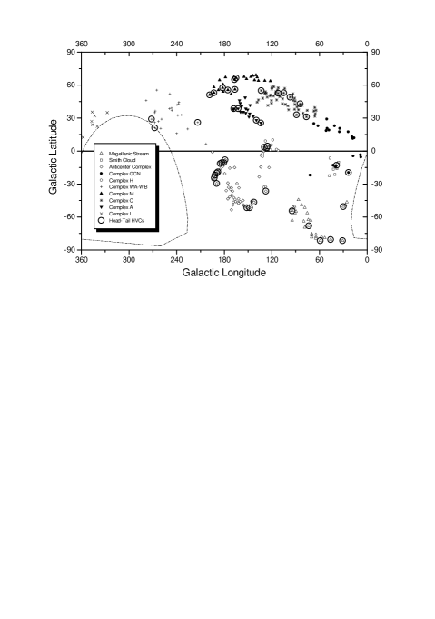
Figure 1: The distribution of the individual HVCs of our sample. Each marker represent an individual HVC of our sample. In total 252 HVCs are identified. The HVCs showing a head-tail structure are indicated by a superposed open circle. The dashed line indicates the southern limit of the LDS at $\delta$ = -30°.

The aim of the present work is to perform a systematic search for HVCs with a head-tail structure in the entire data base of the LDS (Brüns bruens (1998)). For a statistical analysis we need a well defined and representative sample. Therefore we define three conditions which all have to be fulfilled by the HVCs under consideration.

• We identify H i emission lines as high-velocity H i profiles if their radial velocities are at least $|v_{\rm LSR}|\geq$ 90 $\rm km\leavevmode\nobreak\ s^{-1}$and deviate at least 50 $\rm km\leavevmode\nobreak\ s^{-1}$  from a simple galactic rotation model (the second condition is important for areas near the Galactic Plane).

• The HVC must be traceable within three individual H i spectra, to overcome residual baseline uncertainties and broad but faint residual interference signals. We demand further that the signal is not correlated with the observational grid. The minimum three H i spectra are discarded if they are aligned only in galactic longitude or latitude. Accordingly, the three spectra build up the smallest allowed map of a HVC of interest. This corresponds to cloud-sizes larger 1°.

• The minimum H i column density of the studied HVCs is $N_{\rm\hbox{{H {i}}}\leavevmode\nobreak\ }=1\cdot 10^{19}$$\rm cm^{-2}$ . This constraint is introduced to analyze only high-velocity H i profiles with a sufficient signal-to-noise ratio, allowing to study the shape of the H i emission lines in detail.

Applying the three conditions compiled above to the LDS data, we build up a new “bright source catalogue of extended HVCs” for the northern sky offering an angular resolution below $1\degr$.

3.2 General properties of the HVC sample

Fig. 1 shows the distribution of the selected HVCs across the galactic sky. The dashed-dotted line represents the southern declination boundary of the LDS at $\delta=-30\degr$. Each individual marker represents a single HVC selected according to the three criteria mentioned above (Sect. 3.1). In total we identified 252 HVCs. Because of the applied selection criteria, each marker represents a unique line of sight to a HVC. The selected HVCs follow in detail the positional distribution of the well known HVC complexes (Wakker & van Woerden wakker-rev (1997)). The open circles mark the location of HVCs with a head-tail structure (see Sect. 4).

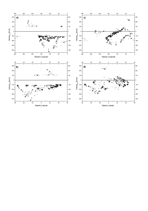
Figure 2: The distribution of the HVCs - radial velocity (in $v_{\rm LSR}$ and $v_{\rm GSR}$) as a function of the parameters galactic longitude and latitude: a $v_{\rm LSR}$ vs. galactic longitude, b $v_{\rm LSR}$ vs. galactic latitude, c $v_{\rm GSR}$ vs. galactic longitude, d $v_{\rm GSR}$ vs. galactic latitude. The transformation from LSR to GSR was calculated according Eq. 1. The HVCs showing a head-tail structure are marked (as in Fig. 1) with open circles.

Figure 3: These histograms show the number of HVCs versus a peak column density, b $v_{\rm LSR}$ and c $v_{\rm GSR}$. The entire HVC sample is plotted in light gray, the HT HVCs are plotted in dark gray. ($\Sigma_{HVC}$ = 252, $\Sigma_{head-tail}$ = 45)

In Fig. 2a the radial velocity (in the local standard-of-rest frame) is plotted versus the galactic longitude. Most of the HVCs have velocities in the range of -200 $\rm km\leavevmode\nobreak\ s^{-1}$$\leq v_{\rm LSR}\leq$ -100 $\rm km\leavevmode\nobreak\ s^{-1}$or +100 $\rm km\leavevmode\nobreak\ s^{-1}$$\leq v_{\rm LSR}\leq$ +200 $\rm km\leavevmode\nobreak\ s^{-1}$. Only HVCs belonging to the Magellanic Stream, the anti-center complex and some clouds near the Galactic Center show radial velocities of v${}_{\rm LSR}\leq$ -200 $\rm km\leavevmode\nobreak\ s^{-1}$. All these more extreme velocity HVCs are located on the southern galactic sky. The absence of a significant number of HVCs with positive radial velocities is because of the limitation to $\delta\geq-30\degr$ of the LDS data. In particular the Magellanic Cloud System is traceable in H i 21-cm line radiation with positive $v_{\rm LSR}$ velocities (see Putman et al. putman (1998) or Putman putman99 (1999) for a recent overview).

Fig. 2b shows the radial velocity (in the local standard of rest) as a function of the galactic latitude. In this figure the north/south asymmetry is visible, i.e. the HVCs in the northern galactic sky have relatively low radial velocities while the HVCs on the southern galactic sky show in general much higher radial velocities.

Figs. 2c and d show our HVC sample in a different representation: radial velocities are transformed into the galactic standard-of-rest frame.

$$v_{\rm GSR}=v_{\rm LSR}+220\leavevmode\nobreak\ {\rm sin}(l){\rm cos}(b)$$ (1)

In Fig. 2c the radial velocity (v_GSR) is plotted versus the galactic longitude. The HVC complexes are grouped now to coherent structures, which are even larger than the extent of an individual HVC complex. For example, the HVC complexes M, A and C build up the largest coherent structure in this representation. Most of the HT HVCs belong to this structure. The Magellanic Stream forms a parallel shifted feature. There is one cloud complex that is clearly outside the main distribution: the Smith cloud (l = 38°, b = –13°, Smith smith (1963)) shows radial velocities v${}_{\rm GSR}\approx$ +250 $\rm km\leavevmode\nobreak\ s^{-1}$while all other clouds have v${}_{\rm GSR}\leq$ +75 $\rm km\leavevmode\nobreak\ s^{-1}$. This may be a hint for a different origin of the Smith cloud. Bland-Hawthorn et al. (bland-hawthorn (1998)) claimed an association of the Smith cloud with the Sgr dwarf.
Fig. 2d shows the radial velocity (v_GSR) as a function of the galactic latitude. The north/south asymmetry is still visible.

Fig. 3 shows histograms of the HVC distribution for the parameters peak column density, $v_{\rm LSR}$ and $v_{\rm GSR}$. The histogram of peak column density versus number distribution of the corresponding HVCs contain information on the studied ensemble. We evaluated the log($N$)-log($S$) correlation (where $N$ is the number of HVCs per flux interval and $S$ is the flux) and found a correlation coefficient of -0.91, clearly indicating a linear relation between both quantities. The linear equation is log($N$) = $(0.53\,\pm\,0.07)\times$ log($S$) +  $(3.00\,\pm\,0.06)$. Within the uncertainties these numbers are equal to the values of Wakker & van Woerden (wakker91 (1991)) on the log($N$)-log($S$) of the population of positive and negative HVCs distributed across the northern sky. This result demonstrates, that our ensemble of HVCs is a representative flux-limited sample of HVCs.
Fig. 3b shows the number distribution with respect to the radial velocity ($v_{\rm LSR}$). Most of the HVCs have velocities in the intervals centered on $v_{\rm LSR}$ = –150 $\rm km\leavevmode\nobreak\ s^{-1}$and –100 $\rm km\leavevmode\nobreak\ s^{-1}$. Fig. 3c shows the number distribution with respect to the velocity ($v_{\rm GSR}$). The bulk of the studied HVCs reveal low radial velocities with respect to the galactic standard of rest frame. The mean $v_{\rm GSR}$ velocity is negative ($\overline{v_{\rm HVC}}$ = –62.3 $\rm km\leavevmode\nobreak\ s^{-1}$$\pm$ 7.5 $\rm km\leavevmode\nobreak\ s^{-1}$), indicating that the majority of HVCs in our sample are moving towards the Galactic Disk. Wakker & van Woerden (wakker91 (1991)) showed that the inclusion of the southern hemisphere H i data on HVCs in their sample does not change this general $v_{\rm GSR}$ velocity behavior.

4 Head-Tail structures

Our HVC sample, selected according to the conditions compiled in Sect. 3, provide information on the distribution of the HVCs relative to the observational parameters galactic longitude and latitude, radial velocity ($v_{\rm LSR},\leavevmode\nobreak\ v_{\rm GSR}$) and peak column density.

In the following step we analyze each individual HVC of the sample with respect to the shape of its H i line profiles, for instance for the variation of the mean velocity and the variation of the column density across the HVC extent.

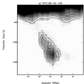
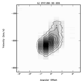
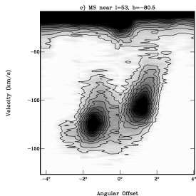
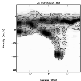
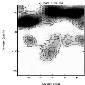
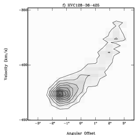
Figure 4: Examples of HVCs with a head-tail structure. These position-velocity diagrams are oriented along the velocity gradient axis of each head-tail HVC: a HVC192-24-130, b HVC189-30-205, c two clouds in the Magellanic Stream (near l=53°, b=–80°.5, d HVC166+56-130 e HVC112+53-150 and f HVC128-36-425; the contour lines start at T_B = 0.21 K (3$\sigma$) in steps of $\Delta$T_B = 0.14 K(2$\sigma$), gray-scale indicates T_B, the darker the color the higher T_B (each Fig. has the same intensity scale). The contour lines in f start at T_B = 0.12 K (3$\sigma$ at $\Delta$v = 3$\rm km\leavevmode\nobreak\ s^{-1}$) in steps of $\Delta$T_B = 0.08 K(2$\sigma$).

4.1 Velocity gradients

We find that about 40% of the HVCs show up with a significant velocity gradient. These velocity gradients are very frequently associated with a column density gradient (20%). The detected velocity gradients are by them-self not a priori indicators for an intrinsic distortion of the HVC velocity field. There are several effects that can produce a velocity gradient.

• The HVCs of our sample are, because of the applied selection criteria, extended objects. Accordingly, the angle between the line of sight and the solar velocity vector varies across the extent of the HVC. This effect can produce a velocity gradient of about 10 $\rm km\leavevmode\nobreak\ s^{-1}$/${\rm[\degr]}$.

• The same kind of velocity gradient is also expected from the HVC velocity vector, because the angle between the HVC velocity vector and the line of sight changes with position, too. This velocity gradient depends on the unknown 3D velocity of a HVC.

• Two or more HVCs may be superposed on the same line of sight with comparable group velocities. The probability for an accidental superposition of two independent HVCs is very low. Nevertheless it is known that HVCs consist of several clumps. The superposition of two clumps that belong to the same HVC has a much higher probability. High angular resolution H i studies may disclose this kind of arrangement.

• Even if there is no evidence for a rotating HVC so far, a rotating HVC would show up with a velocity gradient similar to rotation curves of galaxies. Revealing a red- and blue-shifted extension in the position-velocity diagram.

The effect related to the solar velocity vector is well defined and therefore easy to calculate according to Eq. 1. All other velocity gradients are related to the HVC phenomenon.

4.2 Definition of head-tail structures

Our aim was to search for real distortions in the velocity field of individual HVCs, which may be an indicator for an interaction of the HVC with the surrounding interstellar medium. Accordingly, we studied those HVCs which reveal a velocity and a column density gradient simultaneously. This kind of HVC appears like a comet in the position-velocity domain, and justifies the name head-tail HVC (HT HVC). The head is the region with the highest column density of the HVC, while the column density of the tail is in general much lower (by a factor of 2 - 4). Fig. 4 shows six examples of the studied HT HVCs: the HVC shown in Fig. 4a and b belong to the anti-center complex (HVC189-30-205 and HVC192-24-130). In Fig. 4c two HVCs of the Magellanic Stream are displayed. Both show a head-tail structure. The HVC displayed in Fig. 4d (HVC166+56-130) is a special HT HVC, because the HVC appears to be connected with the H i gas in the Galactic Disk; it forms a so called velocity bridge. Up to now it is unknown, whether the HVC gas is really physically connected to the Galactic Disk gas or just an accidental superposition on the same line of sight. Fig. 4e shows a HT HVC where the head has a relatively low intensity. Fig. 4f shows the HT HVC with the highest observed radial velocity in our sample (v_LSR = –425 $\rm km\leavevmode\nobreak\ s^{-1}$). The velocity resolution was reduced to 3 $\rm km\leavevmode\nobreak\ s^{-1}$in this picture to give an idea of the extent of the tail. This HVC is a very-high-velocity cloud (VHVC) several degrees away from the galaxy M33 (–300 $\rm km\leavevmode\nobreak\ s^{-1}$$\leq$ v${}_{\rm LSR}(\rm M33)\leq$ –75 $\rm km\leavevmode\nobreak\ s^{-1}$).

Figure 5: Correlation between the fraction of HT HVCs on all HVCs of the sample in a certain column density interval versus the peak column density. The solid line marks the result of a weighted linear regression.

4.3 Results

In total, we found 45 HVCs associated with a HT structure in our HVC-sample containing 252 individual HVCs. The column density contrast between the head and the tail varies in general between factors 2 – 4. It is a general behavior that the column density maximum, the head, is located at higher radial velocities than the tail. The HT HVCs are extended objects and cover in general several square degrees.

Fig. 1 shows the distribution of the head-tail HVCs across the galactic sky. The HT HVCs are marked by open circles. Obviously all HVC complexes reveal HT HVCs, even in the northern part of the Magellanic Stream HT HVCs are present. Only in HVC complex L no HT HVCs were found. Fig. 2 shows the distribution of the HT HVCs in comparison to the HVC sample in respect to the parameters galactic longitude, latitude and radial velocity ($v_{\rm LSR}$ and $v_{\rm GSR}$).

In Fig. 3 histograms are plotted for the whole HVC sample and the HT HVCs with respect to the parameters peak column density, $v_{\rm LSR}$ and $v_{\rm GSR}$. We discuss these histograms further in the following subsections.

4.3.1 Peak column density

Fig. 3a shows histograms for the number of HVCs per column density interval. The histogram for the entire HVC sample is plotted in light gray, the histogram for the HT HVCs is plotted in dark gray. It is obvious that there are only relatively few HT HVCs at lower column densities (relative to the HVC sample).
A detailed analysis of the histogram for the peak column density revealed a linear relation between the fraction of head-tail HVCs and the peak column density. Fig. 5 shows this relation. The vertical error-bars are calculated with respect to the low statistics (there are very few HT HVCs with a high column density), the horizontal error-bars indicate the size of the individual $N_{\rm\hbox{{H {i}}}\leavevmode\nobreak\ }$ intervals. The solid line represents the linear regression fit:

$$\frac{\#HTs}{\#HVCs}=(0.0317\pm 0.0028)\frac{N(\hbox{{H {i}}}\leavevmode\nobreak\ )}{[10^{19}{\rm cm^{-2}}]}+$$

$$+(0.017\pm 0.012)$$ (2)

We like to emphasize that the lower limit of $N_{\rm\hbox{{H {i}}}\leavevmode\nobreak\ }=1\leavevmode\nobreak\ 10^{19}$$\rm cm^{-2}$ was chosen to derive statistical significant information on even the faintest HVCs in our sample (this limit is about a factor of 3 above the detection limit using the highest velocity resolution $\Delta$v = 1.03 $\rm km\leavevmode\nobreak\ s^{-1}$of the LDS data). The correlation displayed in Fig. 5 is not biased by a detection limit.
This empirical relation can be used to determine an expected number of HT HVCs for each individual HVC-complex in our sample. The comparison of the expected numbers of HT HVCs with the detected ones shows a good consistency. Only towards the Galactic Anti-Center a significantly larger number of HT HVCs is detected than expected. The correlation explains why we were not able to find HT HVCs in Complex L: this complex has only very few, faint HVCs (the expected number of HT HVCs for this complex is only 0.3).

4.3.2 Radial velocity ($v_{\rm LSR}$)

Fig. 3b shows histograms for the number of HVCs per velocity ($v_{\rm LSR}$) interval. The histogram for the entire HVC sample is plotted in light gray, the histogram for the HT HVCs is plotted in dark gray.
A large number of HT HVCs have radial velocities in the intervals centered on –100 and –150 $\rm km\leavevmode\nobreak\ s^{-1}$(62.2%). This is consistent with the fact that most HVCs have radial velocities in this regime (62.9%). The interval centered on –200 $\rm km\leavevmode\nobreak\ s^{-1}$contains a relatively large fraction of HT HVCs. The large number is expected because of the fact that there is a high percentage of high column density HVCs in this velocity interval, increasing the probability to detect a HT HVC according to Eq. 2. It remains unclear whether there are too many high column density HVCs or too few low column density HVCs in this velocity interval.

4.3.3 Radial velocity ($v_{\rm GSR}$)

Fig. 3c shows histograms for the number of HVCs per velocity ($v_{\rm GSR}$) interval. The histogram for the entire HVC sample is plotted in light gray, the histogram for the HT HVCs is plotted in dark gray.
The mean radial velocity $v_{\rm GSR}$ of the HT HVCs is more negative than the mean radial velocity of the HVC sample. A Gaussian fit to the histograms revealed mean velocities of $\overline{v_{\rm HTHVC}}$ = –86.1 $\rm km\leavevmode\nobreak\ s^{-1}$$\pm$ 3.8 $\rm km\leavevmode\nobreak\ s^{-1}$and $\overline{v_{\rm allHVC}}$ = –62.3 $\rm km\leavevmode\nobreak\ s^{-1}$$\pm$ 7.5 $\rm km\leavevmode\nobreak\ s^{-1}$. The difference between the mean velocities ($\Delta$v=23.8$\rm km\leavevmode\nobreak\ s^{-1}$) is significant. The probability to find a HT HVC increases with negative GSR velocity. We checked that this result is not caused by the relation shown in Fig. 5.
The velocity dispersion in Fig. 3c is nearly identical for the HT HVCs (FWHM = 174.0 $\rm km\leavevmode\nobreak\ s^{-1}$$\pm$ 7.5 $\rm km\leavevmode\nobreak\ s^{-1}$) and the complete HVC sample (FWHM = 179.9 $\rm km\leavevmode\nobreak\ s^{-1}$$\pm$ 15.1 $\rm km\leavevmode\nobreak\ s^{-1}$).

5 Discussion

In the following subsections we discuss possible interpretations for HVCs with a head-tail structure at different distances from the Galactic Disk.

5.1 HVCs in the gaseous Galactic halo

The gaseous halo of the Milky Way has a vertical scale height of 4.4 kpc (Kalberla & Kerp kalberla (1998)). At least the HVC complexes M (z $\leq$ 3.5 kpc, Danly et al. danly (1993), Keenan et al. (keenan (1995)) and Ryans et al. (ryans (1997))) and A (2.5 $\leq$ z $\leq$ 7 kpc, van Woerden et al. van Woerden (1999)) are located within the gaseous halo. As a natural consequence some kind of interaction is expected when a cloud has a high velocity relative to the ambient medium. In a ram-pressure model the head is the interacting HVC and the tail is gas which was recently stripped off from the HVC. In an absolutely homogeneous halo medium there should be a constant interaction rate for all HVCs with similar distances and velocities. The HVC complexes form coherent structures in position and in velocity, i.e. they may form also coherent structures in space. Therefore one would expect naively that all HVCs of a complex should show up with a head-tail structure. This is obviously not observed.
Kalberla & Kerp kalberla (1998) estimate that $\approx$ 10 % of the halo gas is neutral, having higher density than the surrounding plasma. This implies that only those HVCs are expected to show up with a head-tail structure that are passing through an area with locally higher halo density. Accordingly there is a 10 % probability for the creation of a HT HVC. Thus at least 10 % of the HVCs should have a head-tail structure.

In the following we estimate the life-time of a head-tail structure. The HVC tails have on the average a column density of a few times $10^{19}$ $\rm cm^{-2}$ . Because of the low dust abundance in galactic HVCs (in particular in case of the galactic HVC complex M, Wakker & Boulanger wakker86 (1986)) photoelectric heating can be neglected as an excitation process. Only the diffuse X-ray radiation of the galactic halo and the cosmic-rays heat the HVCs. According to Wolfire et al. (wolfirea (1995)a and b) column densities of a few $N_{\rm\hbox{{H {i}}}\leavevmode\nobreak\ }\sim 10^{19}$ $\rm cm^{-2}$ have a high ionization probability. This corresponds to a life-time in the neutral state of about $10^{5}$ – $10^{6}$ years. Compared to the free-fall time of a galactic HVC, of about $10^{7}$ years, the life-time of the stripped-off matter is very short. The tail of a high peak column density HVC contains more material and will survive significantly longer against the ionizing radiation of the diffuse X-rays and cosmic rays. This is consistent with the observational fact that the high peak column density HVCs reveal much more frequently a HT HVC (Fig. 5).
In addition, it is possible that the production or the life-time of a tail depends on the small scale structure of a HVC. HVCs consist of two components: cold clumps are surrounded by an envelope of warm gas. HT HVCs with clumps in their tails will survive much longer than tails that contain only diffuse warm gas. The angular resolution of the LDS is too low to resolve the inner parts of the HVCs. H i observations with high angular resolution are mandatory to study the effects of the small-scale structure.

5.2 The Magellanic Stream

The Magellanic Stream (MS) is the only HVC complex with a generally accepted origin: it is build up by gaseous debris caused by the tidal interaction between the Magellanic Clouds and the Milky Way. The distance of the southern end of the Magellanic Stream is assumed to be very similar to the distance to the Magellanic Clouds (D $\approx$ 50 kpc). In the opposite, the distance of the northern end is unknown. If it is located at low z-heights, i.e. in the gaseous halo, the observed head-tail structures may be produced by the same process as the HT HVCs in the complexes M and A. In this scenario the MS covers a large distance bracket of several tens of kpc. There should be no head-tail structures in the southern part of the stream. On the other hand, the northern part of the MS could have distances similar to the distance of the Magellanic Clouds. The existence of HT HVCs cannot be explained by an interaction with the gaseous halo, because it would be far outside the gaseous halo. A possible interaction partner could be the debris from previous revolutions of the Magellanic System. The ionizing radiation field is much weaker at these distances. Accordingly, the life-time of a tail in the MS is orders of magnitudes longer compared to HVCs in the lower Galactic halo.

5.3 HVCs at extragalactic distances

There is evidence that some HVCs are at intergalactic distances (Braun & Burton braun (1999), Blitz et al. blitz (1999), Sembach et al. sembach (1999)).
Sembach et al. (sembach (1999)) found highly ionized high-velocity gas clouds. Several lines of evidence, including very low thermal pressures (P/k $\approx$ 2 cm^-3 K), favor a location for the highly ionised high-velocity gas clouds in the Local Group or very distant Galactic halo.
Braun & Burton (braun (1999)) searched for compact, isolated HVCs. They classified HVCs as compact if they have angular sizes less than 2 degrees FWHM. They are isolated in that sense, that they are are separated from neighboring H i emission by expanses where no emission is seen to the detection limit of the data. They found 66 of these compact, isolated HVCs. A comparison between their and our sample reveal that the sample of Braun & Burton is much more uniformly distributed in the parameter space (position vs. velocity) than the HVCs of our sample. The different distributions may be an indication for different objects in origin and evolution. Braun & Burton claimed, that their HVCs are most likely located at intergalactic distances. The HVCs of our sample probably contain a significant number of HVCs located in the gaseous halo of the Milky Way. 11 HVCs of their sample are also included in our sample. Moreover, two of them show up with a head-tail structure (HVC271+29+181 and HVC30-51-119).
If these HVCs are located in the intergalactic space, the life-time of the head-tail structures would be much longer because of the much weaker ionizing radiation field at these distances. On the other hand, it is not straight forward to explain what kind of interaction process may produce the observed features at distances of several hundreds of kpc. Especially these (probably very distant) head-tail HVCs should be observed with a higher angular resolution in the near future.

6 Summary and conclusion

We performed a systematic analysis of the HT HVCs across the whole sky that is covered by the LDS (about 75% of the entire sky). We selected a representative flux limited HVC sample with column densities $N_{\rm\hbox{{H {i}}}\leavevmode\nobreak\ }\geq 1\leavevmode\nobreak\ 10^{19}$$\rm cm^{-2}$ and minimum angular diameter $\geq$ 1°. In total we found 252 HVCs.

Each individual HVC was analyzed with respect to velocity gradients and asymmetries in the H i line profiles. The so called head tail HVCs have a cometary shape in the position-velocity domain. We found that 45 out of 252 HVCs show up with a head-tail structure. These HT HVCs are randomly distributed over the whole sky covered by the LDS.

A statistical evaluation of the HVC ensemble revealed that the probability to detect a HT structure increases linear with the peak column density and with increasing negative radial velocity in the GSR frame. There is no significant correlation between the other parameters like galactic longitude, latitude and $v_{\mathrm{LSR}}$.

The detection of HT HVCs in nearly all prominent HVC complexes implies qualitatively comparable physical processes in all of the HVC complexes. Individual HVC cores seem to interact with their ambient medium. In case of the HVC complexes located within the Galactic halo and the Magellanic Stream the interaction with the gaseous halo medium or gaseous debris distributed along the orbit of the Magellanic Clouds may serve as a straight forward explanation for the existence of the HT HVC. At intergalactic distances the detection of HT HVCs is difficult to interpret, because the characteristic time-scale for heating and cooling of the HVC matter is orders of magnitude shorter than the assumed age of these HVC complexes.

High angular resolution H i observations of the detected 45 HT HVCs in future will improve our knowledge on the temperature structure and small-scale column density distribution of this special kind of HVCs. In addition the comparison with other wavelengths, e.g. with H$\alpha$ emission, will help to understand the existence of HT HVCs.

- (1) Bland-Hawthorn J., Veilleux S., Cecil G.N., Putman M.E., Gibson B.K., Maloney P.R., 1998, MNRAS 299, 611
- (2) Blitz L., Spergel D.N., Teuben P.J., Hartmann Dap, Burton W.B, 1999, ApJ 514, 818
- (3) Blom J.J., Bloemen H., Bykow A.M. et al., 1997, A&A 321, 288
- (4) Braun R., Burton W.B., 1999, A&A 341, 437
- (5) Brüns C., 1998, Diploma thesis, University of Bonn
- (6) Danly L., Albert C.E., Kuntz K.D., 1993, ApJ 416, L29
- (7) Hartmann D., 1994,Ph.D. thesis, University of Leiden
- (8) Hartmann D., Kalberla P.M.W, Burton W.B., Mebold U. , 1996, A&AS 119, 115
- (9) Hartmann D., Burton W. B., 1997, “An atlas of Galactic Neutral Hydrogen Emission”, Cambridge University Press
- (10) Herbstmeier U., Mebold U., Snowden S.L., et al., 1995, A&A 298, 606
- (11) Kalberla P.M.W., Kerp J., 1998, A&A 339, 745
- (12) Kalberla P.M.W., Mebold U., Reich W., 1980, A&A 82, 275
- (13) Keenan F.P., Shaw C.R., Bates B., Dufton P.L. Kemp S.N., 1995, MNRAS 272, 599
- (14) Kerp J., Burton W.B., Egger R., et al., 1999, A&A 342, 213
- (15) Meyerdierks H., 1991, A&A 251, 269
- (16) Muller C.A., Oort J.H., Raimond E., 1963, C.R. Acad. Sci. Paris 257, 1661
- (17) Pietz J., Kerp J., Kalberla P.M.W. et al., 1996, A&A 308, L37
- (18) Putman M.E., 1999, astro-ph 9909080, chapter for the book ”High-Velocity Clouds” (Kluwer: Dordrecht), edited by H. van Woerden, U. Schwarz, B. Wakker and K. de Boer
- (19) Putman M.E., Gibson B.K., Staveley-Smith L., et al., 1998, Nat 394, 752
- (20) Ryans R. S. I., Kenan F. P., Sembach K. R., Davies R. D., 1997, MNRAS 289, 83
- (21) Sembach K.R., Savage B.D., Lu L., Murphey E.M. 1999, ApJ 515, 108
- (22) Smith G., 1963, Bull. Astron. Inst. Netherlands 17, 203-208
- (23) Tufte S.L., Reynolds R.J., Haffner L.M., 1998, ApJ 504, 773
- (24) Wakker B.P., Boulanger F, 1986, A&A 170, 84
- (25) Wakker B.P., van Woerden H., 1991, A&A 250, 509
- (26) Wakker B.P. van Woerden H., 1997 A&AR 35, 217
- (27) Weiner B.J., Williams T.B., 1996, AJ 111, 1156
- (28) van Woerden H., Schwarz U.J., Peltier R.F., Wakker B.P., Kalberla P.M.W., 1999, Nat 400, 138
- (29) Wolfire M.G., McKee C.F., Hollenbach D., Tielens A.G.G.M. , 1995a, ApJ 453, 673
- (30) Wolfire M.G., Hollenbach D., McKee C.F., 1995b, ApJ 443, 673