The Sunyaev-Zel’dovich Effect in Abell 370

Abstract

We present interferometric measurements of the Sunyaev-Zel’dovich (SZ) effect towards the galaxy cluster Abell 370. These measurements, which directly probe the pressure of the cluster’s gas, show the gas distribution to be strongly aspherical, as do the x-ray and gravitational lensing observations. We calculate the cluster’s gas mass fraction in two ways. We first compare the gas mass derived from the SZ measurements to the lensing-derived gravitational mass near the critical lensing radius. We also calculate the gas mass fraction from the SZ data by deprojecting the three-dimensional gas density distribution and deriving the total mass under the assumption that the gas is in hydrostatic equilibrium (HSE). We test the assumptions in the HSE method by comparing the total cluster mass implied by the two methods and find that they agree within the errors of the measurement. We discuss the possible systematic errors in the gas mass fraction measurement and the constraints it places on the matter density parameter, $\Omega_{M}$.

to appear in Astrophysical Journal v538 Aug 1, 2000

1 Introduction

Clusters of galaxies, by virtue of being the largest known virialized objects, are important probes of large scale structure and can be used to test cosmological models. Rich clusters are extremely massive, $\sim$$\ 10^{15}M_{\odot}$, as indicated by the presence of strongly gravitationally lensed background galaxies and by the deep gravitational potential necessary to explain both the large velocity dispersion ($>$ 1000 km s^-1) in the member galaxies and the high measured temperature ($>5$ keV) of the ionized intracluster gas. Dynamical mechanisms for segregating baryonic matter from dark matter on these mass scales are difficult to reconcile with observations and standard cosmological models, and so within the virial radius the mass composition of clusters is expected to reflect the universal mass composition. Under the fair sample hypothesis, a cluster’s gas mass fraction, which is a lower limit to the its baryonic mass fraction, is then a lower limit to the universal baryon fraction, i.e., $f_{gas}\leq f_{B}$.

The luminous baryonic content of galaxy clusters is mainly contained in the gaseous intracluster medium (ICM). The gas mass is nearly an order of magnitude larger than the mass in optically observed galaxies (e.g., White et al. 1993, Forman & Jones 1982). Hence, the gas mass is not only a lower limit to the cluster’s baryonic mass, it is a reasonable estimate of it.

The intracluster medium has largely been studied through observations of its x-ray emission. The ICM is hot, with electron temperatures, $T_{e}$, from $\sim$5 to 15 keV; rarefied, with peak electron number densities of $n_{e}\simeq 10^{-3}$ ${\rm cm}^{-3}$; and cools slowly ($t_{cool}>t_{Hubble}$), mainly via thermal Bremsstrahlung in the x-ray band. The x-ray surface brightness is proportional to the emission measure, $S_{x}\propto\int n_{e}^{2}\Lambda(T_{e})dl$, where the integration is along the line of sight, and so, under simplifying assumptions, the gas mass can be calculated from an x-ray image deprojection and the measured gas temperature. Since the sound crossing time of the cluster gas is much less than the dynamical time, one may reasonably assume that, in the absence of a recent merger, the cluster gas is relaxed in the cluster’s potential. The total binding mass can be extracted from the gas density and temperature distribution under this assumption. A significant body of work exists in which the gas mass fraction, $f_{g}$, is measured in this way, with $f_{g}$ measurements out to radii of 1 Mpc or more (White & Fabian 1995; David et al. 1995; Neumann & Bohringer, 1997; Squires et al. 1997; Mohr, Mathiesen & Evrard 1999). The mean cluster gas mass fraction within approximately the virial radius was calculated in Mohr et al. (1999) to be (0.0749 $\pm 0.0005)h^{-3/2}$. Here, and throughout the paper, we assume the value of the Hubble constant to be $H_{\circ}=100h$ km s^-1 Mpc^-1.

To derive the gas mass fraction from x-ray imaging data, one is required to deproject the surface brightness into a model for the density distribution. As the x-ray emission is proportional to the square of the gas density, the gas mass measurement can be biased by clumped, multi-phase gas, should it be present. Also, the emission from the cores of relaxed clusters may be dominated by cooling flows, which complicate the interpretation of the x-ray data and may bias the result strongly if not taken into account (Allen 1998; Mohr et al. 1999). In addition, the x-ray surface brightness is diminished in proportion to its distance; $S_{x}\propto 1/(1+z)^{4}$, where $z$ is the redshift of the cluster, neglecting experiment-specific K-corrections, and so it becomes increasingly difficult to make sensitive x-ray measurements of the ICM as the cluster redshift increases. We present a scheme for measuring the gas mass fractions with the Sunyaev-Zel’dovich effect which is different from the x-ray method in a number of ways, and also provides an independent measurement of $f_{g}$.

The Sunyaev-Zel’dovich (SZ) effect is a spectral distortion of Cosmic Microwave Background (CMB) radiation due to scattering of CMB photons by hot plasma (Sunyaev & Zel’dovich 1970). The SZ effect can be detected significantly in galaxy clusters, where the ionized intracluster gas serves as the scattering medium. A small fraction, $\leq 1\%$, of CMB photons are inverse-Compton scattered and, on average, gain energy. At frequencies less than about 218 GHz, the intensity of the CMB radiation is diminished as compared to the unscattered CMB, and the SZ effect is manifested as a brightness temperature decrement towards the cluster. This decrement, $\Delta T_{SZ}$, has a magnitude proportional to the total number of scatterers, weighted by their associated temperature, ${\Delta T_{SZ}\over T_{CMB}}\propto\int n_{e}T_{e}dl$, where $n_{e}$ is the number density of electrons, $T_{e}$ is the electron temperature, $T_{CMB}$ is the temperature of the CMB, and the integration is again along the line of sight. Note that this is simply proportional to the integrated electron pressure. Also, the magnitude of the SZ decrement is independent of redshift, so as the long as the cluster is resolved (the experiment’s characteristic beamsize is not larger than the angle subtended by the cluster), the SZ effect can be measured towards arbitrarily distant clusters.

A cluster’s gas mass is directly proportional to its integrated SZ effect if the gas is isothermal. So under the isothermality condition, an image deprojection is not strictly required to obtain the gas mass. The cluster’s gas mass fraction can be calculated by comparing the integrated SZ decrement, in effect a surface gas mass, to the total cluster mass in the same volume. The total mass can be measured with strong or weak gravitational lensing, for example. The SZ images may also be deprojected to infer the three-dimensional gas mass and the HSE mass. Since the SZ decrement is directly propotional to the electron density, the SZ image deprojection will not be affected strongly by clumped gas. Thus, the cluster’s gas mass fraction can then be measured as a function of cluster radius as well.

Recent cluster gas mass fraction measurements from SZ effect observations are presented in Myers et al. (1997). In this work, the integrated SZ effect is measured using a single radio dish operating at centimeter wavelengths. The integrated SZ effect is used to normalize a model for the gas density from published x-ray analyses, and this gas mass is compared to the published total masses to determine the gas mass fraction. For three nearby clusters, A2142, A2256 and the Coma cluster, Myers et al. find a gas mass fraction of $(0.061\pm 0.011)h^{-1}$ at radii of 1-1.5 $h^{-1}$ Mpc; for the cluster Abell 478, they report a gas mass fraction of $(0.16\pm 0.014)h^{-1}$.

In this work, we describe a method to calculate cluster gas mass fractions from interferometric SZ observations. Here, the shape parameters are derived directly from the SZ dataset rather than from an x-ray image. We apply this method to the SZ effect measurements towards the cluster Abell 370, which were made as part of an SZ survey of distant clusters, the first results of which were reported in Carlstrom, Joy & Grego (1996), and are further reported in Carlstrom et al. (1997). We choose this primarily because it has been studied at optical and x-ray wavelengths, and so allows a comparison of the SZ data with other observations. Upon detailed investigation, it is apparent that this cluster is one of the most difficult in our sample to analyze, with significant ellipticity and complicated optical and x-ray structure; as such, it serves as a test of the gas mass fraction analysis method, which we plan to use on a large sample of clusters.

With the interferometric SZ measurements, complemented by observations at other wavelengths, we measure the cluster’s gas mass fraction in two ways. First, we calculate the surface gas mass from the SZ measurements and the surface total mass from strong gravitational lensing observations and models. Second, we measure the gas mass fraction in a manner similar to x-ray analyses. The gas mass is inferred from a deprojected model; the total mass is determined from the spatial distribution of the gas under the isothermal hydrostatic equilibrium (HSE) assumption. We test the assumptions made in the HSE analysis by comparing the total cluster masses derived in the two methods.

The optical and x-ray observations of this cluster are discussed in Section 2, and the SZ observations are discussed in Section 3. The method for modeling the SZ data is presented in Section 4, and the gas mass fraction results and the systematic uncertainties are discussed in Section 5. The cosmological implications of the results and plans for future work are discussed in Section 6.

2 Optical and X-ray Observations

The spatial distribution and redshifts of a number of Abell 370’s constituent galaxies have been measured optically. Mellier et al. (1988), using their 29 best galaxy spectra, find Abell 370 has a mean redshift z = 0.374 and velocity dispersion $\sigma_{v}=1340^{+230}_{-150}\ {\rm km\ s^{-1}}$. These observations also show that the cluster is dominated by two giant elliptical galaxies, at ($\alpha_{J2000}=02^{h}\ 39^{m}\ 52.7^{s}$, $\delta_{J2000}=-01^{\circ}\ 34^{\prime}\ 20.3^{\prime\prime}$) and ($\alpha_{J2000}=02^{h}\ 39^{m}\ 53.2^{s}$, $\delta_{J2000}=-01^{\circ}\ 34^{\prime}\ 57.6^{\prime\prime}$), with a projected separation of about $40^{\prime\prime}$ in the north-south direction. The major axes of these two dominant galaxies are also oriented nearly north–south. The Mellier et al. optical isopleth map shows two density peaks, with similar north-south orientation, although these are not centered on the two elliptical galaxies. The 29 galaxy velocities do not appear to be distributed in a Gaussian manner, although the statistics on this modest sample are not conclusive. Should this be significant, its may suggest that the cluster is bimodal or that it is not yet fully relaxed, and the assumption of a simple one-component model in hydrostatic equilibrium would not be appropriate. The mean velocities in the two isopleth peaks are not found to differ significantly, however, nor are the calculated barycenters of the two peaks, and so it is difficult to make a firm conclusion on the state of the cluster based on these data alone.

Abell 370 was the first cluster found to have an associated strongly gravitationally lensed arc $(z_{arc}=0.725$; Soucail et al. 1988). In addition to this giant arc, which apparently consists of multiple images of a single source, three faint pairs of images, each pair presumed to be lensed images of a single galaxy (Kneib et al. 1993), and a radial arc (Smail et al. 1996) have been found to be associated with this cluster. Gravitational lens models have been used to map the total mass distribution in the core region of Abell 370. Kneib et al. (1993) find the position and elongation of the giant arc and the positions of the multiple images are best reproduced by a bimodal distribution of matter, with the two centers of mass nearly coincident with the cluster’s two large elliptical galaxies. A subsequently discovered radial arc is consistent with this model without modifications (Smail et al. 1996).

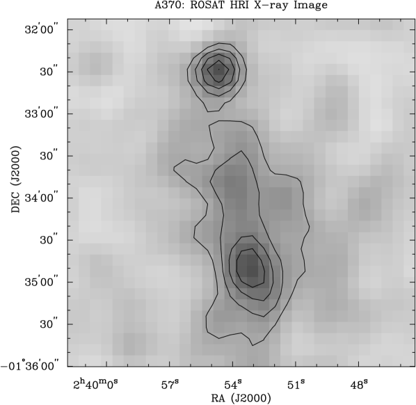
Figure 1: X-ray image of the galaxy cluster Abell 370 observed with the ROSAT HRI. The x-ray image was filtered to include only PHA channels 1-7, binned in 8^′′ x 8^′′ pixels, and smoothed with an 10^′′ Gaussian filter. The background level is 2.8 x 10^-3 HRI counts sec^-1 arcmin ^-2 and the countour levels are at 5.8, 7.2, 8.7, 9.5, 10.1, and 11.6 x 10^-3 HRI counts sec^-1 arcmin ^-2. The x-ray emission peak is associated with a pointlike source located $\sim 2.5^{\prime}$ to the north of the cluster center.

Abell 370 was observed with the High Resolution Imager (HRI) of the ROSAT x-ray satellite. In the ROSAT bandpass (0.1-2.4 keV), x-ray Bremsstrahlung emission from a plasma at gas temperatures typical of clusters depends only weakly on the gas temperature. In Figure 1, we show an HRI image of A370, the result of $\sim$ 30 kiloseconds of observation time. The bright source to the north, at $\alpha_{J2000}=02^{h}\ 39^{m}\ 55^{s}$, $\delta_{J2000}=-01^{\circ}\ 32^{\prime}\ 33^{\prime\prime}$, is coincident with what appears in the Digital Sky Survey to be a nearby elliptical galaxy, NPM1G -01.0096 (Klemola, Jones & Hanson 1987), and does not appear to be associated with A370. The image indicates that the intra-cluster medium also is elongated in the north-south direction, and the emission is strongly peaked at the position of the southern dominant elliptical galaxy, numbered 35 in Mellier et al. (1988), and is offset from the center of the large scale emission. The cluster gas distribution does not appear clearly bimodal at this resolution.

We determine the x-ray surface brightness from the ROSAT HRI image, which has been filtered to include only PHA channels 1-7 in order to reduce the background level (David et al. 1997) and blocked into 8${}^{\prime\prime}\times$ 8^′′ pixels. A circular region with a radius of 24^′′ centered on the pointlike x-ray source to the north of the cluster was excluded from our modeling. We fit a $\beta$-model to the data; this model described in more detail in Section 4, which parametrizes the x-ray surface brightness with a core radius, $\theta_{c}$, and a power law index, $\beta$. The surface brightness of a spheroidally symmetric, isothermal gas distribution will have elliptical contours, and so we also fit for the axis ratio.

We find the best-fit axis ratio of the x-ray image to be 0.73$\pm 0.03$, with major axis exactly north-south, and the center position to be $\alpha_{J2000}=02^{h}\ 39^{m}\ 53^{s}$, $\delta_{J2000}=-01^{\circ}\ 34^{\prime}\ 33^{\prime\prime}$. The best fitting shape parameters for the elliptical model are $\beta$= 0.70$\pm 0.03$ and $\theta_{c}$= 85.0$\pm 3.5^{\prime\prime}$. If the axis ratio is set to equal 1.0, the best fitting shape parameters are $\beta$= 0.72$\pm 0.03$ , $\theta_{c}$= $(70.1\pm 3.2)^{\prime\prime}$ (90% confidence on a single parameter).

Abell 370 was also observed with the Einstein IPC for 4000 seconds. In the IPC image, the northern point source is not apparent. This may be because the FWHM of the instrument point spread function is about 90^′′ at the middle of the 0.4-4.0 keV spectral range of the instrument. (It improves to about 60^′′ at higher energies.) The point source is offset by less than 120^′′ from the center of the extended emission, and so may not be resolved in this image. It may also be explained by source variation; if the point source is an AGN, its surface brightness may have significantly varied between the 1979 IPC observation and the 1994-1995 HRI observations. The image looks less elliptical than does the HRI image, but because the point source emission cannot be excluded from the cluster emission in the IPC data, it is not useful for constraining the spatial distribution of the cluster gas.

Abell 370 has also been observed with the ASCA x-ray satellite. Using 37.5 kiloseconds of ASCA GIS/SIS observations, Mushotzky & Scharf (1997) determined the emission-weighted average temperature of the cluster to be $7.13^{+1.05}_{-0.83}$ keV. Analyzing the same data, Ota, Mitsuda, & Fukazawa (1998) find the emission-weighted temperature to be $6.6^{+1.1}_{-0.9}$ keV. Both of these values are systematically lower than the value obtained in the first analysis of these data by Bautz et al. (1994), who obtain a value of $8.8\pm 0.8$ keV. The discrepancy is presumably because the Mushotzky et al. and Ota et al. analyses used the values of the response matrices of the ASCA telescope and x-ray detectors which have been refined since the Bautz et al. analysis (M. Bautz, private communication). For our analysis, we adopt the Ota et al. value of $6.6^{+1.1}_{-0.9}$ keV, because this published analysis includes detailed discussion of the spectral fitting procedure.

The bright point source evident in the ROSAT HRI image has not been removed from the ASCA spectra in any of the three published analyses. If this emission originates in Bremsstrahlung emission from hot gas in the elliptical galaxy, its characteristic temperature is expected to be less than 1 or 2 keV (Sarazin & White 1988 and references therein). Since the sensitivity of ASCA is optimized for higher energies than this, we would not expect the measured temperature to be greatly contaminated. We assess whether the source is extended, and find that it is pointlike at the resolution of the HRI with a 2.4 $\sigma$ certainty. As the source is unresolved, this emission is also consistent with a galactic cooling flow; if this were the case, the temperature again shouldn’t be greatly contaminated. Should the emission originate from an AGN in the galaxy, though, the effect on the measured temperature is more difficult to predict, and will depend strongly on the index of the power law of the AGN spectrum.

Without further measurements, we cannot rule out that the cluster’s spectrum is contaminated by emission from an AGN. It is also possible that if the cluster is in fact bimodal with two distinct subclusters, the measured emission-weighted average $T_{e}$ will be a value between the temperatures of the two subclusters. Lacking more definitive measurements, we continue with our assumption that the gas is isothermal at $kT=6.6^{+1.1}_{-0.9}$ keV. The estimated effects of the described uncertainties on the results are discussed in Section 5.3.

We compare A370’s measured line-of-sight velocity dispersion with our adopted gas temperature, and find $\beta_{spec}\equiv{\mu m_{p}\sigma^{2}_{v}}/{{kT_{e}}}=1.87^{+1.02}_{-0.59}$. If the energy per unit mass contained in the galaxies is equal to that in the gas, and the cluster is spherical, we expect $\beta_{spec}$ to be $\sim 1$. If the temperature measurement is biased low, e.g., from an AGN, this will contribute to the $\beta_{spec}$ discrepancy. Elongation of the cluster potential along the line of sight or a alignment of two (or more) subclusters will also enhance the measured $\beta_{spec}$.

The optical and x-ray observations suggest that A370 is not a relaxed cluster, and may be heavily substructured, but due to insufficient signal-to-noise ratios and contaminating sources, these observations still leave some ambiguity.

3 SZ Observations

We observed Abell 370 for 50 hours over nine days with the Owens Valley Radio Observatory (OVRO) Millimeter Array in 1996 August and 43 hours over six days with the Berkeley-Illinois-Maryland Association (BIMA) Millimeter Observatory in 1997 June-August. We set our pointing center to $\alpha_{J2000}=02^{h}\ 39^{m}\ 52.5^{s}$, $\delta_{J2000}=$ $-01^{\circ}\ 34^{\prime}\ 20^{\prime\prime}$, the position of the northern dominant elliptical galaxy.

We outfitted the millimeter telescopes with centimeter-wavelength receivers to broaden the instrument’s angular resolution to the large angular scales typical of clusters. The receivers are based on low noise High Electron Mobility Transistor (HEMT) amplifiers (see Pospieszalski 1995), operating from 26 to 36 GHz. The single-mode receivers are constructed to respond only to circularly polarized light. The receivers interface with each array’s delay lines and correlator. The standard observational scheme entailed interleaving 20 minute cluster observations with observations of a strong reference source near the cluster, which allows monitoring of the instrumental amplitude and phase gain. The amplitude gain drifts were minimal; the gain changes were less than a percent over a many hour track, and the average gains were quite stable from day to day. The amplitude gains were calibrated by comparing the measured flux of Mars with that predicted by the Rudy model for Mars’ whole disk brightness temperature (Rudy, 1987) at the observed frequency and the apparent size of Mars as indicated by the Astronomical Almanac. The Rudy model is a radiative transfer model with an estimated accuracy of 4% (90% confidence) at centimeter wavelengths. Data taken when the projected baseline was within 3% of the shadowing limit were not used.

The OVRO Millimeter array consists of six 10.4 meter telescopes. The OVRO continuum correlator was used to correlate two 1 GHz bands centered at 28.5 GHz and 30 GHz. The system temperatures ranged from 40-60 K, depending on elevation and atmospheric water content. The primary beams of the telescopes were measured holographically and can be approximated as Gaussian with a full width at half maximum (FWHM) of 252^′′. The data were calibrated and edited using the MMA data reduction package (Scoville et al. 1993) taking care to remove data taken during poor weather or which show any anomalous phase jumps.

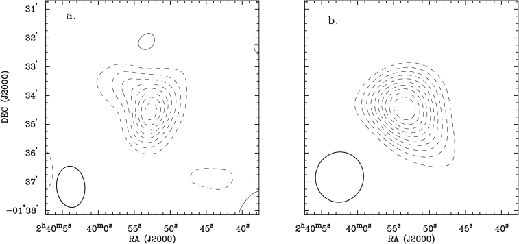
Figure 2: a. Image of Abell 370 from OVRO observations. The restoring beam, shown in the lower left hand corner, has a Gaussian FWHM of $59^{\prime\prime}$ x $86^{\prime\prime}$. The RMS noise in the map is 50 $\mu$Jy beam^-1, or 14.9 $\mu$K, and the integrated flux density of the source is $-1.54\pm 0.17$ mJy. b. Image of A370 from BIMA observations. The restoring beam has FWHM of $91^{\prime\prime}$ x $95^{\prime\prime}$. The RMS noise in the map is 180 $\mu$Jy beam^-1, or 31.4 $\mu$K, and the integrated flux density of the source is $-4.34\pm 0.52$ mJy.

We image the data using the DIFMAP package (Shepard, Pearson, & Taylor 1994). Examining images of A370 made with projected baselines greater than 2.0 $k{\lambda}$, we find a point source 45^′′ to the east of the map center (map center is the pointing center) in both continuum bands. Its measured flux density in the 28.5 GHz band, attenuated by the instrumental primary beam pattern, is +0.69 $\pm$ 0.10 mJy and is +0.84 $\pm$ 0.10 mJy in the 30 GHz band. This source, 0237-0147, is discussed further in Cooray et al. 1998. We combine the two continuum channels, and find the best fitting model is a point source with flux density of $0.725\pm 0.07$ mJy. The point source model is removed from the $u$-$v$  or spatial frequency, data set in order to construct the SZ decrement map. A Gaussian taper with FWHM of 1.2 $k\lambda$ is applied in the $u$-$v$ plane to the combined dataset and map was CLEANed, restricting the CLEAN components to the central 200^′′, about the size of the decrement in the primary. The map presented in Figure 2a is made with a restoring beam of Gaussian FWHM $59^{\prime\prime}$ x $86^{\prime\prime}$, with contour intervals of 1.5 $\sigma$. The $rms$ noise in the map is 50 $\mu$ Jy beam^-1, or 14.9 $\mu$K, and the integrated flux density of the source is $-1.54\pm 0.17$ mJy.

We employed nine of the 6.1 meter telescopes of the BIMA array for SZ observations, using the same centimeter-wave receivers we used at OVRO. We center the 800 MHz bandwidth of the BIMA digital correlator at 28.5 GHz. We achieved system temperatures of 30-55 K, scaled to above the atmosphere, depending on elevation and atmospheric water content. Holographic antenna pattern measurements were also made with this system. The primary beam at BIMA is nearly Gaussian with a $396^{\prime\prime}$ FWHM. The data were edited and reduced using the MIRIAD data reduction program (Sault, Teuben & Wright 1995), taking care to the remove any spurious interference from the spectral channels and dropping the low signal-to-noise channels at the spectral filter edges.

Again using DIFMAP, we find the same point source at about $45^{\prime\prime}$ to the east of the pointing center in a high resolution (projected baselines longer than $1.4~{}k\lambda$) image. The point source measured at BIMA in 1997 has flux density of +0.70 $\pm$ 0.17 mJy. The primary beam attenuation at the point source position in the BIMA system is $\sim 6\%$ less than the attenuation at this position at OVRO, and so the point source observations are consistent with the flux being constant in time. We model and subtract the point source from the data set, apply a Gaussian taper with FWHM of 0.8 $k\lambda$ in the $u$-$v$ plane and construct a map of the decrement. The map was CLEANed, restricting the CLEAN components to the central $\sim 300^{\prime\prime}$ of the image, about the size of the primary beam. The restoring beam used to make the map in Figure 2b. is a Gaussian with FWHM $91^{\prime\prime}$ x $95^{\prime\prime}$, and the contours presented are at intervals of 1.5 $\sigma$. The $rms$ noise in the map is 180 $\mu$Jy beam^-1, or 31.4 $\mu$K, and the integrated flux density of the source is $-4.34\pm 0.52$ mJy.

It is instructive to compare the general characteristics of the SZ images to the x-ray map. At the resolution of both the OVRO and BIMA instruments, the gas is extended in the north-south direction, though less markedly than in the x-ray map. The substructure suggested by the lensing and velocity dispersion data is not evident here. We produce maps from each of the datasets, increasing the image resolution, but the gas still does not show significant substructure or bimodality. The SZ decrement distribution is not peaked at the pointing center, but south of it, at a position about halfway between the two elliptical galaxies (this will be quantified in the next section). The detailed appearance of the SZ map, especially the shapes of the least significant contours, depends on the specific method of point source removal and the CLEANing of the data, and so it is not useful to compare the spatially filtered and CLEANed SZ and x-ray images at such a level of detail. As we will discuss in the following section, the quantitative analysis of the SZ data is done using the $u$-$v$ data directly.

4 Modeling

In order to assess the data more quantitatively, we fit a parametrized model to the SZ brightness distribution. Since the SZ data are taken in the spatial frequency, or $u$-$v$, domain, we do the model comparisons in $u$-$v$ domain as well.

We measure the SZ temperature decrement in units of antenna temperature, $T_{a}$, which relates an observed intensity change to a Rayleigh-Jeans temperature change, $\Delta I_{\nu}={2k\nu^{2}\over c^{2}}\Delta T_{a}$. In order to recover the true blackbody temperature decrement, the $\Delta T_{RJ}$ measured and reported here should be multiplied by a factor of 1.021, as we are not strictly in the Rayleigh-Jeans limit. The SZ temperature decrement, ${\Delta T_{SZ}}\over{T_{CMB}}$, is proportional to the Compton $y$-parameter,

$$y={{k\sigma_{T}}\over{m_{e}c^{2}}}\int{n_{e}(l)T_{e}(l)dl},$$ (1)

where $k$ is Boltzmann’s constant, $\sigma_{T}$ is the Thomson scattering cross section, $m_{e}$ is the electron mass, $n_{e}$ is the electron density, $T_{e}$ is the electron gas temperature, and the integral extends along the line of sight ($dl$). The proportionality depends on the observing frequency; it depends also on the electron temperature when relativistic corrections are included (Rephaeli 1995, Challinor & Lasenby 1998).

At 28.5 GHz, ${\Delta T_{RJ}\over T_{CMB}}=-1.92$ $y$ in the non-relativistic Rayleigh-Jeans approximation, where we adopt the value of the CMB of Fixsen et al. (1996) derived from the COBE FIRAS measurements, $T_{CMB}=2.728$ K. Including the relativistic corrections for $kT_{e}=6.6$ keV, ${\Delta T_{SZ}\over T_{CMB}}=-1.86\ y$.

We fit a simple model to the SZ data. The $\beta$-model (Cavaliere & Fusco-Femiano 1976, 1978) is frequently used to fit the density profiles of galaxy clusters. The spherically symmetric, isothermal $\beta$-model describes $n_{e}$, the density distribution of the gas, as varying as a function of cluster radius, $r$:

$$n_{e}(r)=n_{e\circ}\left(1+{r^{2}\over r_{c}^{2}}\right)^{-3\beta/2},$$ (2)

where $n_{e\circ}$ is the number density of the gas at the center of the spheroidally symmetric gas distribution; $r_{c}$, the core radius, is a characteristic size of the cluster; and $\beta$ is the power law index.

Since the cluster appears elliptical in projection, we generalize the spherically-symmetric $\beta$-model and allow the gas density profile to be spheroidally symmetric, i.e., with biaxial symmetry. In the spheroidally symmetric model, the electron number density in a prolate spheroid is a function of $\eta^{2}=r^{2}+a^{2}z^{2}$, where $r$ and $z$ are the radial and height coordinates in the cylindrical coordinate system, and $a<1$ is the axis ratio of the two unique axes. If the spheroid is oblate, then the density is a function of $\eta^{2}=a^{2}r^{2}+z^{2}$, with $a<1$. The electron density then follows the distribution:

$$n_{e}(\eta)=n_{e\circ}\left(1+{\eta^{2}\over r_{c}^{2}}\right)^{-3\beta/2},$$ (3)

If the cluster gas is isothermal and its symmetry axis is in the plane of the sky, this electron density distribution leads to the following two-dimensional SZ temperature decrement:

$${\Delta T}\left(\theta\right)=\Delta T(0)\left(1+{\theta_{\eta}^{2}\over\theta_{c}^{2}}\right)^{{1\over 2}-{3\beta\over 2}},$$ (4)

where $\theta_{\eta}=\eta/D_{A}$, $D_{A}$ is the angular diameter distance, $\theta_{c}=r_{c}/D_{A}$, and $\Delta T(0)$ is the temperature decrement at zero projected radius,

$${\Delta T(0)\propto T_{e}n_{e\circ}\int\left(1+\left({l\over r_{c}}\right)^{2}\right)^{-{3\over 2}\beta}dl},$$ (5)

where the integral, $dl$ is along the line of sight. Formally, this integral extends from the observer along the line of sight through the cluster infinitely; in practice, a cutoff radius for the cluster is used. The $\beta$-model distribution of the electron density projects to a $\beta$-model distribution of the SZ decrement if the system obeys spherical or ellipsoidal symmetry.

We perform a $\chi^{2}$ analysis of the $\beta$-model, by comparing $\beta$-models to the combined BIMA and OVRO datasets. We vary the following parameters: centroid position, $\beta$, $\theta_{c}$, axis ratio (defined to be $<$ 1), position angle (defined counter clockwise from north), and $\Delta T(0)$. The position and flux density of the radio-bright point source are also fit. The fitting procedure is conducted in several steps. The model corresponding to each set of the seven cluster fit parameters and the three point source parameters is multiplied by the primary beam response. The Fourier transform of the result is compared directly with the interferometer data. We use the holographically determined primary beams when modeling the data, and the entire datasets are used to do the analysis. The inner $u$-$v$ radius cutoff is determined by the shadowing limit, the limit where one telescope would partially block another, i.e., when the projected baseline is less than the diameter of a telescope dish. For the BIMA data this limit is $0.58\ k\lambda$ and for the OVRO data it is $1\ k\lambda$. The $\chi^{2}$ statistic is minimized, and the best fit values are determined using a downhill simplex method.

Performing the fitting procedure, we find the best fit parameter values for A370 are: $\theta_{c}$ = $93^{\prime\prime}$, $\beta$ = 1.77, $\Delta T(0)$ $=-609$ $\mu K$, and axis ratio = 0.64 with major axis exactly north-south. The best fit central position is $20^{\prime\prime}$ to the south of the pointing center, at $\alpha_{J2000}=02^{h}\ 39^{m}\ 53.2^{s}$, $\delta_{J2000}=-01^{\circ}\ 34^{\prime}\ 40.4^{\prime\prime}$, about halfway between the two giant elliptical galaxies, and 7^′′ north of the fitted centroid for the x-ray image. The $\chi^{2}$ statistic for the best fit values is 135798 for 136136 degrees of freedom, yielding a reduced $\chi^{2}$ of 0.9975. As points of comparison, we fit to the data a null model for the cluster (with the point source component), which gives a reduced $\chi^{2}$ of 0.9986; we also fit the cluster to a negative point source, finding a reduced $\chi^{2}$ of 0.9986.

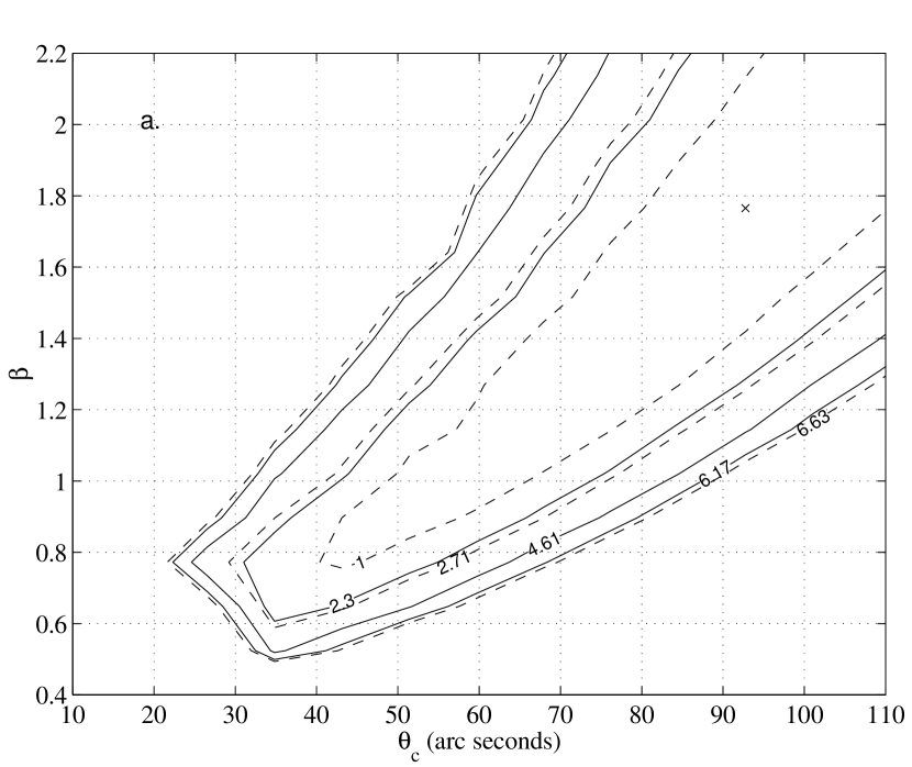
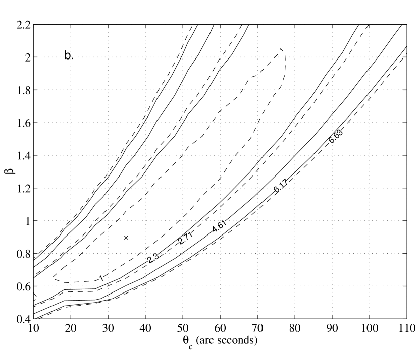
Figure 3: Confidence regions from the joint fit to the BIMA and OVRO SZ data using a. an elliptical $\beta$-model and b. a spherical $\beta$-model. In both plots, the best fit ($\beta$, $\theta_{c}$) point is indicated with an x and the full line contours show the $\Delta\chi^{2}$ = 2.3, 4.61, and 6.17 regions, which indicate 68.3%, 90.0%, and 95.4% confidence, respectively, for the two-parameter fit. The dashed lines show $\Delta\chi^{2}$ $=$1.0, 2.71, and 6.63 regions; the projection of these regions onto the $\beta$ or $\theta_{c}$ axis indicate the 68.3%, 90% and 99% confidence interval on the single parameter. The centroid and point source flux and position are fixed at the best fit values, and $\Delta T(0)$ is allowed to assume its best fit value at each ($\beta$, $\theta_{c}$) point.

In order to determine the uncertainties in these fitted parameters, the $\chi^{2}$ statistic is derived for a large range of $\beta$, $\theta_{c}$, and $\Delta T(0)$, keeping centroid position, position angle, and point source position and flux fixed to the best fit values. Presented in Figure 3a is a contour plot of the $\beta$ and $\theta_{c}$ fit results, where $\Delta T(0)$ is allowed to assume its best fit value at every pair of $\beta$ and $\theta_{c}$. The axis ratio is left to assume its best fit value at each set of $\beta$, $\theta_{c}$, and $\Delta T(0)$; it varies from 0.60 to 0.68 for points with $\Delta\chi^{2}$ $<$ 5 from the best fit point. The centroid position, when left to assume its best fit value at each point, does not appreciably change, varying less than 5^′′. Figure 3b shows the contours derived when fitting the data to a spherical model for the gas distribution, i.e., the axis ratio is fixed to a value of 1.0; in this case, the best fit parameter values are $\theta_{c}$ = $34^{\prime\prime}$, $\beta$ = 0.86, $\Delta T(0)$ $=-785$ $\mu K$, the reduced $\chi^{2}$ statistic was 0.9976.

The full line contours are marked for $\Delta\chi^{2}$  = 2.3, 4.61, and 6.17 which indicate 68.3%, 90.0%, and 95.4% confidence, respectively, for the two-parameter fit. The dashed lines indicate $\Delta\chi^{2}$ $=1.0$, 2.71, and 6.63; the projection onto the $\beta$ or $\theta_{c}$ axis of the interval contained by these contours indicate the 68.3%, 90% and 99% confidence interval on the single parameter. The values of $\Delta T(0)$ for which $\Delta\chi^{2}$ $<$ 1 at each ($\beta$, $\theta_{c}$) point range about 15% from the best fit value. This illustrates that $\beta$ and $\theta_{c}$ are correlated strongly and are not individually well constrained by these data. This poor constraint is at least partly due to the low declination of A370, which makes sampling non-redundant spatial frequencies difficult at OVRO and BIMA. The shape parameters fit from the x-ray data are not consistent with those from the SZ data. This could be a result of shocks and complexity in the gas phase which affect the x-ray emission and SZ effect differently. This discrepancy is difficult to resolve with the information at hand; for the purpose of the next section, investigating the gas mass fraction of the cluster using the SZ effect, we use the SZ fitted parameters only.

We also fit the data with a $\beta$-model which includes a truncation of the gas distribution at a given radius. With truncation radii from 300^′′ to 1000^′′, the shape parameters ($\beta$, $\theta_{c}$, $\Delta T(0)$) best fit values do not change appreciably, much less than the variation contained within the $\Delta\chi^{2}$ $<$ 1 region. The $\chi^{2}$ statistic changes only minimally for different cutoff radii, with $\Delta\chi^{2}$ less than 0.1. This indicates that the possible systematic uncertainty in the fitted parameters due to modeling the data without a cutoff is not significant.

Since the optical and x-ray data suggest that Abell 370 may have a bimodal gravitational potential, we also fit the data with a pair of circular $\beta$-models, each allowed independent shape parameters and position. The best fit two-component model has one component centered at $\sim 50^{\prime\prime}$ south of the pointing center, 10^′′ south of the large southern elliptical galaxy; the best fit position of the second component is $\sim 5^{\prime\prime}$ north of the pointing center, i.e., $5^{\prime\prime}$ north of the large northern elliptical. The southern component has best-fit parameters $\beta$ = 0.65, $\theta_{c}$= 10^′′, and $\Delta T(0)$ = $-765$ $\mu$K; the northern component has best-fit parameters $\beta$ = 0.83, $\theta_{c}$ = 27^′′, and $\Delta T(0)$ = $-605$ $\mu$K. Adding a second component reduces the $\chi^{2}$ statistic by 2 when 3 new parameters are introduced (compared to the single $\beta$-model with axis ratio and position angle free), and therefore is not a significantly better fit to the data. Allowing the axis ratios of the two components to vary does not improve the fit.

5 Analysis

5.1 Comparison of SZ Gas Mass to the Strong Lensing Mass Estimate

As indicated by Equation 1, the SZ brightness at any point in the two-dimensional projected image is simply proportional to the integrated electron density along the line of sight, if the gas is isothermal. Under the isothermal assumption, we can directly measure the total number of electrons in the gas contained in the cylindrical volume of a chosen radius, the long axis of which is defined by the line of sight. The total mass in the ionized phase can be calculated from this assuming a value for the number of nucleons per electron. If the gas has solar metallicity, as measured by Anders & Grevesse (1989), the nucleon/electron ratio is 1.16. The nucleon/electron ratio changes less than 1% for values of the metallicity from 0.1 to 1.0.

The interferometric measurements recover much of the total SZ decrement on the angular scales measured, i.e.  the integrated flux from the data comprises 40-50% (depending on the instrument) of the integrated flux in a best fit model to these data. And so the unmodeled interferometer data provides a strong lower limit to the integrated SZ decrement at the angular scales of interest. The model is fitted to the $u$-$v$ data in order to estimate the full, two-dimensional decrement, and thence the surface gas mass. This method does not assume anything about the state of the ICM other than that it is isothermal.

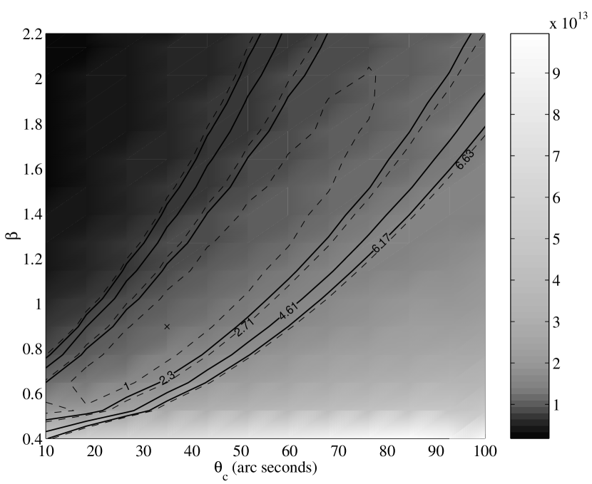
Figure 4: Gas Mass for Abell 370. The gas mass in a cylindrical volume with cross section of 65^′′ and axis ratio 0.64, in units of $M_{\odot}$ is shown in greyscale. The two-parameter confidence intervals for $\beta$ and $r_{c}$ are overlaid. At each point, $\Delta T(0)$ assumes its best fit value. The best fit point is marked with an x.

We fit the SZ data in the three-dimensional parameter space 0.4 $<\beta<$ 4.0, 10${}^{\prime\prime}<r_{c}<$250^′′, $-2000$ $\mu$K $<\Delta$T(0) $<$ $-200$ $\mu$K, both for elliptical and circular models. At each $\beta$, $\theta_{c}$, and $\Delta T(0)$ point, we calculate the surface gas mass and the $\chi^{2}$ statistic, from which confidence limits for the surface gas mass are determined. Although the 68% confidence region contains a large range of $\beta$ and $\theta_{c}$ values within 68% confidence, as was evident in Figure 3, the gas mass, which depends on all three gridded parameters, is constrained relatively well. In Figure 4, we show the derived surface gas mass at radius 65^′′ as it varies with $\beta$ and $\theta_{c}$ in the circular $\beta$-model fitting. The gas mass in this geometry is $1.5^{+0.7}_{-0.6}\times 10^{13}h^{-2}M_{\odot}$. The temperature decrement is allowed to assume its best fit value at each point for this figure, although for the quantitative analysis, the full range of $\Delta T(0)$ is used. The isomass surfaces, shown in greyscale, follow the shape of the confidence interval contours, indicating that sets of parameters which fit the data well will predict the same gas mass. This is to be expected, since under the isothermal assumption, the SZ flux is directly proportional to the gas mass, and the fit parameters must reproduce the same observed flux at the angular scales where the flux is best measured.

We derive a surface gas mass to compare with the lensing mass using our fitted model parameters. The lensed arc in Abell 370 has a radius of curvature of about 30^′′ centered nearly halfway between the dominant galaxies; this center is at about the same position of the gas density centroid in the one component $\beta$ model. We calculate the surface gas mass in a cylindrical volume centered at this position and with an elliptical (axis ratio = 0.64) cross-section, using the fits to the elliptical $\beta$-model. We choose a major radius of 40^′′ since the lens model should be most accurate near the lensed arc’s radius. The SZ-derived surface gas mass with the elliptical cross-section is $5.4^{+1.2}_{-1.0}\times 10^{12}h^{-2}M_{\odot}$, at 68% confidence. Included in the error estimates are the uncertainty due to the fit parameters, the SZ absolute calibration uncertainty, and the gas temperature measurement uncertainty. The uncertainty is not appreciably smaller if we restrict the shape parameters to those which typically found in x-ray image analyses of clusters, i.e., $\beta$ $<1.5$. The uncertainties of the masses derived from the elliptical fits are smaller than those from the spherical fits because the confidence contours follow the isomass contours more closely.

We also derive the gas mass in the model with two components. The best fitting two-component $\beta$-model parameters are integrated in a cylinder with radius 40^′′, centered on the centroid of the best fit single component model. This yields a gas mass of $4.84\times 10^{12}h^{-2}M_{\odot}$, consistent with the single component model. Since the bimodal model doubles the parameter space over which fits must be made, making a comprehensive parameter fit unfeasable, we approximate the statistical uncertainty from the fit to be the same as in the single model fit, about 20%.

These surface gas masses are compared to the cluster’s total mass in the same volume implied by the strong gravitational lensing measurements. The surface total mass can be inferred from a model of the cluster mass distribution which predicts the observed gravitational lensing. We calculate the gravitational mass using the lensing model in Kneib et al. (1993) for the same volume, centered at the SZ model fit center. Although the uncertainties on the model parameters are less than ten percent, we make a conservative estimate of 20% for the uncertainty, to allow for variations of this model. Comparing this mass, $9.6^{+1.9}_{-1.9}\times 10^{13}h^{-1}M_{\odot}$, to the single-component gas mass yields a gas mass fraction, $f_{g}$, of $(0.056^{+0.017}_{-0.015})h^{-1}$; the two-component model yields a slightly lower gas mass fraction of $(0.046\pm 0.013)h^{-1}$. The cluster’s angular diameter distance was calculated assuming $\Omega_{M}$ = 0.3 and $\Omega_{\Lambda}$ = 0. If $\Omega_{M}$ = 1.0, $\Omega_{\Lambda}$ = 0, the angular diameter distance to A370 will be 6.5% smaller, as will $f_{g}$. If $\Omega_{M}$ = 0.3 and $\Omega_{\Lambda}$ = 0.7, $f_{g}$ will be $\sim 9\%$ larger.

5.2 Comparison of SZ Gas Mass to Hydrostatic, Isothermal Mass Estimates

Since strong gravitational lensing in clusters is relatively rare and is restricted to the cores of clusters, and weak lensing analyses are published for only selected clusters, we also consider the more general means of calculating the cluster gas fraction, deprojection of the density model and the HSE assumption. We assume the gas is in hydrostatic equilibrium, is isothermal, and is spheroidally symmetric; for simplicity, we assume the symmetry axis is in the plane of the sky. The surfaces of constant electron density are then concentric ellipsoids. We then compare the gas mass and the HSE mass from the deprojected model to determine the gas mass fraction.

Specifically, to determine the gas mass, we extract the central electron density, $n_{e\circ}$, from the deprojected $\beta$-model and measured electron temperature by performing the integral along the line of sight in Equation 5 and integrating Equation 2. We do this for each set of $\beta$, $\theta_{c}$, and $\Delta T(0)$. These calculations require an assumption about the geometry of the cluster, since the core radius and extent of the cluster along the line of sight are not known. For an oblate ellipsoid, the axis of symmetry is the cluster’s minor axis, and the core radius in the line-of-sight direction is equal to the cluster’s observed major axis; for a prolate ellipsoid, the axis of symmetry is the major axis, and the core radius in the line-of-sight direction is equal to the minor axis.

The fit parameters are then used to constrain the total mass. Hydrostatic equilibrium implies

$${{1\over\rho_{gas}}\nabla p_{gas}=-\nabla\Phi},$$ (6)

where $\rho_{gas}$ and $p_{gas}$ are the gas density and pressure, respectively. The cluster’s gravitational potential, $\Phi$, can be related to the total mass density, $\rho_{grav}$, by Poisson’s equation,

$${\nabla^{2}\Phi=4\pi G\rho_{grav}},$$ (7)

where $G$ is the gravitational constant. We can solve for the density of the cluster’s gravitational mass by combining Equations 6 and 7:

$${\rho_{grav}=-{1\over{4\pi G}}\nabla\cdot\left({1\over\rho_{gas}}\nabla p_{gas}\right)}.$$ (8)

We relate the pressure, density, and temperature of the gas through the equation of state:

$${p_{gas}={{\rho_{gas}kT_{e}}\over{\mu m_{p}}}},$$ (9)

where $k$ is Boltzmann’s constant, $\mu$ is the mean molecular weight of the gas, and $m_{p}$ is the proton’s mass. To calculate $\mu$, we again assume the gas has the solar metallicity of Anders and Grevesse (1989) and that $\mu$ is constant throughout the gas. Making the assumption that the gas is isothermal, we write Equation 8 in the form:

$${\rho_{grav}=-{{kT_{e}}\over{4\pi G\mu m_{p}}}\nabla^{2}{\rm ln}\rho_{gas}}.$$ (10)

Note that the gravitational mass density depends only on the shape of the gas distribution, and so is independent of the value of the central gas density and the gas mass fraction. Using the derived shape parameters, $\beta$, $\theta_{c}$, and projected axis ratio, $a$, and the measured gas temperature, we estimate the total mass density of the cluster. We again choose the simplest geometries, that of oblate and prolate ellipsoids, and integrate the density within the same volume as we do the gas density.

For the same range of $\beta$, $\theta_{c}$, and $\Delta T(0)$ as we used in the cylindrical geometry analysis, we calculate the cluster’s ellipsoidal gas mass, HSE mass, and gas mass fraction for both prolate and oblate geometries, and the $\Delta\chi^{2}$ from the best fit parameters. From $\Delta\chi^{2}$ = 1 range of fit parameters, we derive the $68\%$ confidence intervals for the gas mass and the mean gas mass fraction calculated within different major axis radii.

We prefer to measure the masses and mass fractions in the largest volume permitted by our method, since the fair sample assumption is best at large radii and the cores of clusters may be affected significantly by physical processes not included in our HSE model (cooling flows, galaxy winds, magnetic fields). The largest scales on which we make our calculations are determined by the shortest baselines on which we detect the SZ effect. We calculate the statistical uncertainties in the $f_{g}$ measurement due to the shape parameter uncertainties on a number of scales, from 10^′′ to 150^′′. There is a broad minimum in uncertainty around radius 65^′′.

We calculate the gas mass fraction for the oblate and prolate spheroids at semi-major axis $65^{\prime\prime}$ ($\sim 330h^{-1}$kpc). The gas mass is the same for both oblate and prolate geometries; the change in central density and volume when the geometry changes exactly compensate. For the oblate ellipsoid, the gas mass fraction is (0.064${}_{-0.024}^{+0.024})h^{-1}$; for the prolate ellipsoid, the gas mass fraction is (0.096${}_{-0.034}^{+0.036})h^{-1}$. We also calculate $f_{g}$ in a spherical volume of radius $65^{\prime\prime}$, using the fits and uncertainties from the spherical fits and find $f_{g}$ = (0.080${}^{+0.04}_{-0.041})h^{-1}$. The calculated values are compiled in Table 1.

We also calculate the gas mass fraction for both components of the bimodal model, using a gas temperature of 6.6 keV for each and find that the gas mass fraction for each component is $\sim 0.040h^{-1}$.

The dark matter needed to produce concentrically ellipsoidal isopotential surfaces has a significantly more aspherical distribution than the potential. For the observed axis ratio of 0.64, this dark matter distribution is unphysical beyond a few core radii in the direction of the unique axis, as it requires the dark matter density to be negative. This also implies that the gas mass fraction will vary spatially. The difficulty of this model supporting very elliptical gas density distributions may be suggesting that the cluster is bimodal, but it is more likely an indictment of the simplified models we have used. We have considered the class of potentials with isopotential surfaces following concentric ellipsoids because they adequately describe the data and because their deprojections are straightforward. Such simplified models are seriously deficient, however, for the hydrostatic analysis. To produce a cluster with an observed axis ratio of less than $1/\sqrt{2}$ in this formalism, the cluster mass must be partially comprised of dark matter with negative density. It is improper, then, to measure the dark matter with this method out past a few core radii for a highly elliptical cluster.

The effect of using this simple ellipsoidal model to calculate $f_{g}$ is assessed in the following way. We construct a model cluster which has a physically motivated mass structure, predict its observed SZ effect, and then attempt to recover the simulated cluster’s mass using the same observation and analysis protocol used for the true observations. We arrange the dark matter of the simulated cluster in concentrically spheroidal shells with a $\beta$-model profile. The dark matter’s axis ratio is set to 2.0:3.5. Isothermal gas at 7 keV is added in hydrostatic equilibrium with the cluster potential, and a simulated two-dimensional SZ decrement map constructed, assuming the cluster is at redshift $z$ = 0.37. The decrement map is sampled with the $u$-$v$ coverage of a typical interferometric observation. Noise typical of a $\sim$ 40 hour observation is added. The resulting $u$-$v$ data are fit in the same manner described in Section 4, with the data fit to a concentrically ellipsoidal $\beta$-model, and the gas mass and gas mass fraction determined with the HSE method. Two simulations are used, one model cluster is an oblate spheroid and the other a prolate spheroid, both with the symmetry axis in the plane of the sky. In both cases, the best fit axis ratio of the gas distribution was 0.79. These gas masses and gas mass fractions are compared to the actual model values. These are shown in Table 2.

The model appears to be adequate at small radii, but deteriorates noticeably by a radius of 100^′′. This suggests it is reasonable to measure the gas mass fraction with this model near the same radius we constrain the data well. We restrict our analysis of the real observations to within radius of $65^{\prime\prime}(\sim$ 330$h^{-1}$ kpc), a region within which the approximation is valid.

5.3 Systematic Uncertainties

5.3.1 Comparing the Lensing and HSE Masses

If the assumptions made in the hydrostatic isothermal analysis are valid, the HSE predicted mass should equal the cluster’s lensing mass. We integrate the total mass density in Equation 10 in the same cylindrical volume in which the lensing mass is calculated. This comparison is potentially a means to discriminate between oblate and prolate models for the cluster, but, as discussed in Section 5.2, our model for ellipsoidal clusters breaks down at large radii. For the spherical model, this mass is calculated for each set of shape parameters and the 68% confidence limits are derived. Using an electron temperature of $6.6^{+1.1}_{-0.9}$ keV, the spherical geometry HSE mass integrated in the 40^′′ radius cylindrical volume is $1.47^{+0.49}_{-0.38}\times 10^{14}M_{\odot}$, consistent with the lensing mass in the same geometry of $1.59^{+0.30}_{-0.30}\times 10^{14}h^{-1}M_{\odot}$. The two-component $\beta$-model predicts about $1.25\times 10^{14}M_{\odot}$, and so it is also a consistent model.

This agreement does not guarantee that the assumptions in the HSE analysis are valid, however. For this reason, we examine possible systematic effects. Some comparisons of cluster total masses derived by the HSE method to lensing masses suggest that the HSE method systematically underpredicts the cluster’s mass (e.g., Miralda-Escudé & Babul 1994, Loeb & Mao 1994, Wu & Fang 1997). Some of the explanations suggested for the discrepancy include cluster ellipticity, non-thermal pressure support of the gas in the cluster core, multi-phase gas, and temperature gradients in the gas. In an examination of a large sample of clusters, however, Allen (1998) suggests such discrepancies can often be resolved by taking account of cooling flows when analyzing x-ray data, and ensuring that the lensing and x-ray masses probe the same line of sight. The mass discrepancy does remain for clusters in the Allen sample with small cooling flows or none, perhaps suggesting these clusters have undergone recent dynamical activity which have disrupted any pre-existing cooling flow. Such activity might invalidate the HSE assumption.

We have been careful to ensure that the strong lensing and SZ models probe the same lines of sight. There is no evidence for a cooling flow in Abell 370, although there may be other concerns about using the measured emission-weighted gas temperature.

5.3.2 Contamination of Emission-Weighted Temperature

If the measured average temperature is in error, i.e., due to contamination from a nearby AGN, the mass measurements will also be in error. The SZ gas mass is inversely proportional to the assumed temperature and the HSE mass is directly proportional to the temperature. The gas fraction from the HSE method is quite sensitive to temperature, $f_{g}\propto 1/T_{e}^{2}$.

5.3.3 Polytropic Temperature Gradient

An unresolved temperature gradient in the gas may systematically affect the gas and HSE masses. If such a gradient is present, the true temperature in the central region may be higher than the emission-weighted temperature we use, and the fitted shape parameters from the isothermal SZ analysis may no longer accurately describe the density distribution.

However, if the temperature of the intracluster medium declines slowly, and does not change appreciably over the angular scales to which we are sensitive, the interferometric measurement of the gas mass fraction at these angular scales will in fact not be strongly affected.

Currently, there are no strong observational constraints on temperature structure in moderately distant and distant clusters, as there have been no suitable telescope facilities for the task. However, an attempt to quantify temperature structure observed in nearby clusters is presented in Markevitch (1996). In this work, a slow decline in temperature with radius is observed, with the temperature falling to half its central value at 6-10 core radii. This structure may be approximately described by a gas with a polytropic index of $\gamma$ = 1.2. (For discussion of polytropic indices, see Sarazin (1988) and the references within.) If there temperature structure in Abell 370 and it is of the moderate variety presented in Markevitch (1996), it will not be a strong source of systematic uncertainty.

Abell 370 has a long observation scheduled with the Chandra observatory. Chandra has the necessary spatial and spectral resolution to remove the effects of contaminating sources in the field and with a long observation, could measure the spatial variation of the cluster temperature, should it exist.

5.3.4 Inclination Angle

The assumption that the cluster is biaxially symmetric with symmetry axis in the plane of the sky is certainly a simplification. Here, we estimate the effect on the gas mass fraction of an inclined symmetry axis. Analytical relationships between the inclination angle and the apparent shape of an biaxial ellipsoid are derived in Fabricant, Rybicki, & Gorenstein (1984). We derive the cluster gas mass and HSE mass for a cluster which reproduces the observed SZ map, but has an inclined symmetry axis. A biaxial cluster, when inclined, will retain a $\beta$-model distribution with the same value of $\beta$, but the central density and intrinsic axis ratio will change. The inclination angle $i$ is measured between the symmetry axis and the line of sight; $i=90^{\circ}$ for the analysis of Section 5.2.

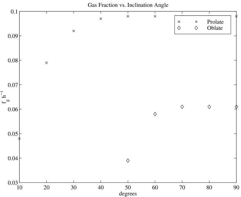
Figure 5: The ellipsoidal gas mass fraction, calculated with the isothermal HSE method, as a function of inclination angle, $i$. The mass is calculated using the best fit parameters from the elliptical $\beta$-model fit.

As inclination angle increases, so does the intrinsic axis ratio. In order to preserve the observed SZ effect, The value of the central density must vary inversely with the axis ratio. The gas mass, then, remains the same for all inclination angles. This is expected, as the gas mass is proportional to the total SZ flux, independent of its spatial arrangement. We evaluate the gas and HSE masses as a function of $i$, using the best fit parameters from A370. The gas mass fraction changes, but it changes significantly over a relatively small range of allowed inclination angles (see Figure 5).

6 Discussion

6.1 Gas Mass Fractions at $r_{500}$

To compare the $f_{g}$ we have measured within a fixed angular radius to $f_{g}$ measurements in clusters with different sizes and redshift, we extrapolate our measured $f_{g}$ to a fiducial radius. The ICM in nearby clusters has been observed to be distributed more uniformly than the dark matter (e.g., David et al. 1995), which is to be expected if energy has been added to the intracluster medium before collapse or from galactic winds. If this is generally true, the gas mass fraction measured depends on the radius within which the measurement is made. As suggested in Evrard (1997) and Metzler, Evrard, & Navarro (1998), we choose this radius to be that within which the average density of the cluster is 500 times the critical density, $\rho_{c}={{3H^{2}}\over{8\pi G}}$. These numerical simulations suggest that within this radius, $r_{500}$, the cluster’s baryon fraction should closely reflect the universal baryon fraction, if the current physical models of hierarchical structure formation are correct. We use the analytical expression of Evrard (1997) which describes the expected variation of $f_{g}$ with overdensity. This variation is found to be consistent with the $f_{g}$ variation reported in the David et al. (1995) sample.

$${f_{g}(r_{500}(T_{e}))=f_{g}(r_{X})\left({r_{500}(T_{e})\over r_{X}}\right)^{\eta}},$$ (11)

where $\eta$ = 0.17, $f_{g}(r_{500}(T_{e}))$ is the gas mass fraction at $r_{500}$, and $r_{X}$ is the radius within which the gas mass fraction is measured. We modify Evrard’s expression for $r_{500}$, derived for low redshift clusters, to include the change in the value of $\rho_{c}$ with redshift; $\rho_{c}(z)=\rho_{c}(z=0)(H/H_{\circ})^{2}$, where $H^{2}=H_{\circ}^{2}[(1+z)^{3}\Omega_{M}+(1+z)^{2}(1-\Omega_{M}-\Omega_{\Lambda})+\Omega_{\Lambda}]$

$${r_{500}(T_{e})=(1.24\pm 0.09)\left({T_{e}\over 10\ {\rm keV}(H/H_{\circ})^{2}}\right)^{1/2}h^{-1}{\rm Mpc}}.$$ (12)

The gas mass fraction values at $r_{500}$, estimated from those measured at 65^′′, are summarized in Table 1.

This experiment best measures $f_{g}$ at a given angular scale, which corresponds in Abell 370 to an overdensity of $\sim 5000\rho_{c}$. This is not the optimal radius at which to compare with numerical simulations, since resolution is limited in the cores of the clusters, and the gas in the core may also be sensitive to additional physics not yet included in the models, e.g., magnetic fields and cooling. For these reasons, the corrections should be taken with some caution.

6.2 Constraints on $\Omega_{M}$ from $f_{g}$

Under the fair sample hypothesis, A370’s gas mass fraction within $r_{500}$, a lower limit to the cluster baryon fraction, should reflect the universal baryon fraction:

$$f_{g}\leq f_{B}={\Omega_{B}\over\Omega_{M}},$$ (13)

where $f_{B}$ is the cluster’s baryon fraction, $\Omega_{M}$ is the ratio of the total mass density to the critical mass density, and $\Omega_{B}$ is the ratio of baryon mass density in the universe to the critical mass density. The cluster gas mass fraction measurements can then be used within the Big Bang Nucleosynthesis (BBN) paradigm to constrain $\Omega_{M}$:

$$\Omega_{M}\leq\Omega_{B}/f_{g}.$$ (14)

The value of $\Omega_{B}$ is constrained by BBN calculations and the measurements of light element abundances. The relative abundance of deuterium and hydrogen provides a particularly strong constraint on the baryonic matter density. A firm upper limit to $\Omega_{B}$ is set by the presence of deuterium in the local interstellar medium. This constrains the value of $\Omega_{B}$ to be less than $0.031h^{-2}$ (Linsky et al. 1995). Measurements of the D/H ratio in metal-poor Lyman-$\alpha$ absorption line systems in high-redshift quasars put a tighter constraint on the baryonic mass density. Such measurements made by Burles & Tytler (1998) predict a value of $\Omega_{B}=(0.019\pm 0.002)h^{-2}$ at 95% confidence.

The gas mass fractions measured for A370 from both lensing and HSE methods range from $5-13\%h^{-1}$. We consider the simplest $f_{g}$ measurement, that in the spherical model, and compare this gas mass fraction at $r_{500}$ to the Burles & Tytler (1998) value for $\Omega_{B}$. This gives an upper limit to the matter density parameter, $\Omega_{M}\leq 0.19^{+0.10}_{-0.10}h^{-1}$, at 68% confidence. However, the bimodal model gives a surface gas mass fraction at angular radius 40^′′ of 0.048$h^{-1}$, a value which permits $\Omega_{M}$ to be as high as 0.40$h^{-1}$ in this scheme. (We note again that the dependence of $f_{g}$ through the angular diameter distance is weak at this redshift, with a change in $f_{g}$ of 5-10% when a wide range of cosmological parameters is used.) These values are consistent with the limits on $\Omega_{M}$ from observations of supernovae, which are derived from geometrical arguments, rather than the $\Omega_{B}/f_{g}$ ratio. Depending on the method used to calibrate the sample, for a spatially flat universe, Garnavich et al. (1998) find $\Omega_{M}$ $<0.4-0.5$ at 68% confidence.

6.3 Conclusion & Future Work

We have measured the Sunyaev-Zel’dovich effect in the galaxy cluster Abell 370 and present spatially filtered images from these data. The optical and x-ray observations of this cluster show a complicated and perhaps bimodal mass distribution. The SZ effect image, however, looks smoothly distributed and significantly aspherical. We have fit both one-component and two-component $\beta$-models to the data and find that the two-component model does not fit significantly better. For both models, we calculate the gas mass fraction for the cluster using measurements of the total cluster mass from both the gravitational lens model (the “surface” gas mass fraction) and from the hydrostatic equilibrium assumption. When integrated in the same volume, the HSE masses are consistent with the mass derived from the gravitational lensing model for both the one- and two-component models, lending support to the HSE assumption. The surface gas mass fraction measurement is made within an angular radius of 40^′′ and the HSE gas mass fraction is made within a radius of 65^′′. The gas mass fraction near the virial radius is derived from the gas mass fractions at 65^′′ using a correction factor derived from numerical simulations. For the range of methods and models used, we find gas mass fraction values of $\sim(5-13)h^{-1}\%$.

Constraints on the Hubble parameter $H_{\circ}$ can in principle be derived from the SZ and x-ray measurements of a cluster. The SZ and x-ray observables depend on different moments of the electron density, and so the characteristic length scale of the cluster along the line of sight can be measured and the angular diameter distance of the cluster inferred. This is useful not only as a distance ladder-independent measurement of $H_{\circ}$, but, when compared with other $H_{\circ}$ measurements, can be used to explore possible systematic effects in the $f_{g}$ calculation, e.g., to constrain the deprojection of the gas distribution. However, the quality of the x-ray imaging data in this case and the apparent disagreement between the SZ and x-ray fitted models do not permit putting a strong constraint on the Hubble constant. A long observation with the Chandra x-ray observatory towards this cluster is planned, and should help resolve these issues.

The value of the baryonic mass fraction in any one cluster will be susceptible to systematic uncertainties which may be difficult to estimate. In order to use cluster gas mass fractions as a cosmological tool, one wants to ameliorate the effect of these errors by studying a large sample of clusters. A SZ effect survey in galaxy clusters is being carried out by this group at the BIMA and OVRO observatories, and an analysis of the gas mass fraction of the sample is in preparation.

Many thanks are due to the staff at the BIMA and OVRO observatories for their contributions to this project, especially Rick Forster, John Lugten, Steve Padin, Dick Plambeck, Steve Scott, and Dave Woody. Many thanks to Cheryl Alexander for her work on the system hardware. Thanks also to Jack Hughes and Doris Neumann for valuable discussions concerning the x-ray analysis, to Jean-Paul Kneib concerning his lensing analysis, and to Naomi Ota and collaborators for sharing their reduced ASCA data. This work is supported by NASA LTSA grant NAG5-7986. LG, EDR, and SKP gratefully thank the NASA GSRP program for its support. Radio astronomy with the OVRO and BIMA millimeter arrays is supported by NSF grant AST 93-14079 and AST 96-13998, respectively. The funds for the additional hardware for the SZ experiment were from a NASA CDDF grant, a NSF-YI Award, and the David and Lucile Packard Foundation.

Table 1: Gas Mass Fractions for Abell 370

geometry	$f_{g}$	$\frac{f_{g}(\delta_{500})}{f_{g}(65")}$	$f_{g}(\delta_{500})$
cylinder (radius=40′′)	$(0.056^{+0.017}_{-0.015})h^{-1}$	…	…
cylinder (radius=40′′), bimodal	$(0.046^{+0.013}_{-0.013})h^{-1}$	…	…
oblate ellipsoid (radius=65′′)	(0.064${}_{-0.024}^{+0.026})h^{-1}$	1.22	(0.078${}_{-0.029}^{+0.032})h^{-1}$
prolate ellipsoid (radius=65′′)	(0.106${}_{-0.044}^{+0.048})h^{-1}$	1.22	(0.129${}_{-0.054}^{+0.059})h^{-1}$
sphere (radius=65′′)	(0.080${}^{+0.044}_{-0.041})h^{-1}$	1.22	(0.098${}^{+0.050}_{-0.054})h^{-1}$

Note. — The surface $f_{g}$ (cylindrical geometry) is derived from the elliptical $\beta$-model (with $a=0.64$) and the two-component model for the SZ effect and the total mass from the strong gravitational lensing model of Kneib et al. (1993). The ellipsoidal gas mass fractions are calculated from deprojections of both the elliptical and spherical $\beta$-model fits to the SZ data and the isothermal HSE assumption. The major axis indicated in the first column and symmetry axes are assumed to be in the plane of the sky. The radius within which $f_{g}$ is measured is indicated in the first column; $f_{g}$ within $r_{500}$ is estimated in Column 4, using a correction factor (Column 3) from Equation 11.

Table 2: Comparison of Derived to True Gas Mass and Gas Mass Fraction

	Within 65′′	Within 100′′
Oblate Cluster, $i=90^{\circ}$
	derived value/true value	derived value/true value
total mass	1.05${}^{+0.08}_{-0.08}$	1.42${}^{+0.16}_{-0.43}$
gas mass	0.98${}^{+0.08}_{-0.08}$	0.96${}^{+0.14}_{-0.12}$
gas mass fraction	0.95${}^{+0.19}_{-0.19}$	0.65${}^{+0.35}_{-0.06}$
Prolate Cluster, $i=90^{\circ}$
	derived value/true value	derived value/true value
total mass	0.88${}^{+0.17}_{-0.17}$	1.16${}^{+0.27}_{-0.14}$
gas mass	0.87${}^{+0.26}_{-0.07}$	0.88${}^{+0.34}_{-0.14}$
gas mass fraction	1.11${}^{+0.62}_{-0.25}$	0.79${}^{+0.87}_{-0.20}$

Note. — We test the effect of using an ellipsoidally symmetric $\beta$-model for the gas density distribution. We simulate SZ observations of an oblate cluster and a prolate cluster and analyze them with the methods of Sections  4 and  5.2. We compare the quantities we derive to the true simulated cluster’s values.

References

- (1) Allen, S. W. 1998, MNRAS, 296, 392
- (2) Anders, E., & Grevesse, N. 1989, Geochimica et Cosmochimica Acta 53, 197
- (3) Bautz, M., Mushotzky, R., Fabian, A., Yamashita, K., Gendreau, K., Arnaud, K., Crew, G., & Tawara, Y. 1994, PASJ, 46, L131
- (4) Burles, S., & Tytler, D. 1998, ApJ, 507, 732
- (5) Carlstrom, J. E., Joy, M. K., & Grego, L. 1996, ApJ, 456, L75
- (6) Carlstrom, J. E., Joy, M. K., Grego, L., & Holzapfel, W. 1997, in Proceedings of the 21st Annual Texas Symposium on Relativistic Astrophysics, ed. Olinto, A. V., Frieman, J. A., & Schramm, D. N. (Singapore: World Scientific Publishing)
- (7) Cavaliere, A., & Fusco-Femiano, R. 1976, A & A, 49, 137 —.1978, A & A, 70, 667
- (8) Challinor, A., & Lasenby, A. 1998, ApJ, 499, 1
- (9) Cooray, A. R., Grego, L., Holzapfel, W. L., Joy, M., Carlstrom, J. E. 1988, AJ, 115, 1388
- (10) David, L. P., Harnden, F. R., Kearns, K. E., Zombeck, M. V., Harris, D. E., Prestwich, A., Primini, F. A., Silverman, J. D, Snowden, S. L. 1997, The ROSAT High Resolution Imager (HRI) Calibration Report, U.S. ROSAT Science Data Center/SAO, 25
- (11) David, L. P., Jones, C., Forman, W. 1995, ApJ, 445, 578
- (12) Evrard, A.E. 1997, MNRAS, 292, 289
- (13) Fabricant, D., Rybicki, G., Gorenstein, Pl 1984, ApJ, 286, 186
- (14) Fixsen, D. J., Cheng, E. S., Gales, J. M., Mather, J. C., Shafer, R. A., & Wright, E. L. 1996, ApJ, 473, 576
- (15) Forman, W., & Jones, C., 1982, ARA&A, 20, 547
- (16) Klemola, A. R., Jones, B. F, Hanson, R. B. 1987, AJ, 94, 501
- (17) Kneib, J., Mellier, Y., Fort, B., & Mathez, G. 1993, A & A, 273, 370
- (18) Linsky, J. L., Diplas, A., Wood, B. E., Brown, A., Ayres, T. R., & Savage, B. D. 1995, ApJ, 451, 335
- (19) Loeb, A., Mao, S. 1994, ApJ, 435, L109
- (20) Markevitch, M., 1996, ApJ, 465, L1
- (21) Mellier, Y., Soucail, G., Fort, B., & Mathez, G., 1988, A & A, 199, 13
- (22) Metzler, C. A., Evrard, A. E., & Navarro, J. F. 1996, ApJ, 469, 494
- (23) Miralda-Escudé, J., & Babul, A. 1995, ApJ, 449, 18
- (24) Mohr, J. J., Mathiesen, B., Evrard, A. E. 1999, ApJ, 517, 627
- (25) Mushotzky, R. F., Scharf, C.A. 1997, ApJ, 482, L13
- (26) Myers, S. T., Baker, J. E., Readhead, A. C. S., & Leitch, E. M. 1997, ApJ, 485, 1
- (27) Neumann, D. M., Bohringer, H. 1997, MNRAS, 289, 123
- (28) Ota, N., Mitsuda, K., & Fukazawa, Y. 1998, ApJ, 495, 170
- (29) Pospieszalski, M. W., Lakatosh, W. J, Nguyen, L. D., Lui, M., Liu, T., Le, M., Thompson, M. A, Delaney, M. J. 1995, Microwave Symposium Digest, IEEE MTT-S International, 3, 1121
- (30) Rephaeli, Y. 1995, Annual Reviews A & A, 33, 541
- (31) Rudy, D. J., 1987, PhD. Thesis, California Institute of Technology
- (32) Sarazin, C. L. 1988, X-Ray Emission from Clusters of Galaxies, Cambridge University Press, Cambridge Astrophysics Series
- (33) Sarazin, C. L., & White, R. E. 1988, ApJ, 331, 102
- (34) Sault, R. J., Teuben, P. J., & Wright, M. C. H. 1995, in Astronomical Data Analysis Software and Systems IV, ed. R. A. Shaw, H. E. Payne & J. J. E. Hayes. PASP Conf Series 77, 433 (1995).
- (35) Scoville, N. Z., Carlstrom, J. E., Chandler, C. J., Phillips, J. A., Scott, S. L., Tilanus, R. P. J., & Wang, Z. 1993, PASP, 105,1482
- (36) Shepherd, M.C., Pearson, T.J., & Taylor, G.B. 1994, BAAS, 26, 987
- (37) Smail, I., Dressler, A., Kneib, J.-P., Ellis, R.S., Couch, W.J., Sharples, R.M., & Oemler, A., Jr. 1996, ApJ, 469, 508
- (38) Soucail, G., Mellier, Y., Fort, B., Mathez, G., Cailloux, M. 1988, A & A, 191 no. 2, L19
- (39) Squires, G., Neumann, D. M., Kaiser, N., Arnaud, M., Babul, A., Bohringer, H, Fahlman, G. 1997, ApJ, 482, 648S
- (40) Sunyaev, R.A., & Zel’dovich, Ya.B. 1970, Comments Astrophys. Space Phys., 2, 66
- (41) White, D. A., & Fabian, A. C. 1995, MNRAS, 273, 72
- (42) White, S. D. M., Navarro, J. F., Evrard, A. E., & Frenk, C. S. 1993, Nature, 366, 429
- (43) Wu, X., & Fang, L. 1997, ApJ, 483, 62
- (44)