Monte Carlo inversion of hydrogen and metal lines from QSO absorption spectra

Abstract

A new method, based on the simulated annealing algorithm and aimed at the inverse problem in the analysis of intergalactic (interstellar) complex spectra of hydrogen and metal lines, is presented. We consider the process of line formation in clumpy stochastic media accounting for fluctuating velocity and density fields (mesoturbulence). This approach generalizes our previous Reverse Monte Carlo and Entropy-Regularized Minimization methods which were applied to velocity fluctuations only. The method allows one to estimate, from an observed system of spectral lines, both the physical parameters of the absorbing gas and appropriate structures of the velocity and density distributions along the line of sight. The validity of the computational procedure is demonstrated using a series of synthetic spectra that emulate the up-to-date best quality data. H i, C ii, Si ii, C iv, Si iv, and O vi lines, exhibiting complex profiles, were fitted simultaneously. The adopted physical parameters have been recovered with a sufficiently high accuracy. The results obtained encourage the application of the proposed procedure to the analysis of real observational data.

1 Introduction

QSO absorption line spectroscopy being a major activity at many observatories for the last two decades is now developing into a powerful tool for extragalactic research thanks to the new generation of large telescopes. The steady improvement in sensitivity and resolution of spectroscopic instrumentation opens new fields in the study of QSO absorption systems. It is now becoming possible to investigate the intensity fluctuations within the line profiles and thus to estimate hydrodynamic characteristics of the absorbing gas.

The majority of the narrow QSO absorption lines represents intervening systems and allows us to probe the properties of diffuse matter at very high redshifts. Resolved profiles of hydrogen lines and especially lines of heavier elements (‘metals’) show a diversity of shapes and structures. Up to now, their analysis is based on the assumption that the observed complexity is caused by individual ‘clouds’ randomly distributed along the line of sight with slightly different radial velocities. It is also a basic assumption that the hydrodynamic (‘bulk’ or ‘turbulent’) velocity distribution inside each cloud is Gaussian and completely uncorrelated (microturbulence). This model implies that each subcomponent of the complex profile being resolved should have a symmetrical profile and its shape should not alter with higher spectral resolution. Observations show, however, that the complexity of the line profiles increases with higher resolution, a tendency expected for correlated bulk motions which have, in general, non-Gaussian distributions along a given line of sight (Levshakov & Kegel 1997; Levshakov, Kegel & Mazets 1997; Levshakov, Kegel & Takahara 1999; Papers I, II, and III hereafter, respectively). It follows that the microturbulent approximation is not appropriate in this case because it does not account for all the relevant physical processes involved in the radiative transfer. Moreover, being applied to real data, the microturbulent analysis leads to a loss of valuable information contained in the observations and may even yield unphysical results (Levshakov & Kegel 1999; Levshakov, Takahara & Agafonova 1999; LTA hereafter). The need for more sophisticated procedures of data analysis becomes therefore obvious.

In recent years, it has been shown that accounting for the correlations in the velocity field (mesoturbulence) may change the interpretation of the line measurements substantially (Papers I and II). A mesoturbulent approach has been already successfully applied to the study of the deuterium and hydrogen absorption in Q 1937–1009 (Levshakov, Kegel & Takahara 1998a), Q 1718+4807 (Levshakov, Kegel & Takahara 1998b), and Q 1009+2956 (Levshakov, Tytler & Burles 2000). For all three QSOs about the same value for the D/H ratio was derived in contrast to the previously announced microturbulent results. Our first inversion codes, – the Reverse Monte Carlo (Paper III), and the Entropy-Regularized Minimization (LTA), – have been developed for a model of a stochastic velocity field neglecting any density fluctuations. They have been applied to the analysis of the H i and D i lines and/or to the metal absorption lines with similar profiles when species trace the same volume elements independently on the density fluctuations. In the present paper, we extend this study to the inverse problem for a model of compressible turbulence when one observes non-similar profiles of different atoms and/or ions from the same absorption-line system. As in our previous papers, we use the term ‘turbulence’ in a wider sense as compared with hydrodynamic turbulence to label the unknown nature of the line broadening mechanism. In this regard we consider any kind of bulk motions (infall, outflows, tidal flows etc.) of more or less stochastic nature leading to fluctuating velocity and density (temperature) fields as continuous random functions of the space coordinate along a given line of sight within the intervening absorbing region.

Two noteworthy works have been recently carried out aiming at the recovery of the physical intergalactic structure from the Lyman-$\alpha$ forest lines. Nusser & Haehnelt (1999a,b) developed an inverse procedure based on the relation between density and velocity Fourier coefficients. The quality of their recovery is, however, restricted by the assumption that the Lyman-$\alpha$ forest structure traces mainly the matter density distribution and that the amplitude of the peculiar velocities is rather small to affect the local absorption coefficient significantly. This assumption is questionable since there is no simple way to distinguish observationally whether the density or the velocity fluctuations are the main source of the ‘line-like’ structure observed in the Lyman-$\alpha$ forest (Levshakov & Kegel 1998). Moreover, recent studies of nearby large-scale motions in the universe indicate that the Hubble flow is considerably perturbed. Peculiar velocities in the range from 300 to 500 km s^-1 have been found in a sample of galaxies complete out to a distance of 60 Mpc (e.g., Watkins 1997; Gramann 1998; Giovanelli et al. 1998), a fact which should be taken into account in the inverse procedures.

The method described in the present paper is quite flexible and equally accounts for the density and velocity fluctuations. It is based on a stochastic optimization approach similar to that developed in Paper III. We estimate simultaneously the physical parameters and appropriate realizations of the density $n(s)$ and velocity $v(s)$ distributions along the line of sight to reproduce hydrogen and metal lines from a given absorption system. In this regard, the more spectra of different elements are incorporated in the analysis the higher accuracy of the estimation can be obtained.

In $\S 2$ our model and the underlying basic assumptions are specified. The inversion code is described in $\S 3$. The validity of the method is tested in $\S 4$ using simulated sets of noisy line profiles (H i, C ii, Si ii, C iv, Si iv, and O vi). Finally, the main conclusions are outlined in $\S 5$.

2 Hydrogen and metal absorption from QSO Lyman-limit systems

In this section we consider the line formation in a Lyman-limit system (LLS), – the intervening absorbing gas being optically thin in the Lyman continuum (presumably outer regions of a foreground galaxy). To specify the calculations, we use the standard photoionization model of Donahue & Shull (1991, hereafter DS), namely, an extended region of thickness $L$ with a given metallicity. The region is ionized by a background photoionizing spectrum given by Mathews & Ferland (1987). The gas is assumed to be in thermal equilibrium.

We concentrate our efforts on the LLSs because, on one hand, they can be analyzed with a minimum number of model assumptions and, on the other hand, they are the most promising targets for measuring the extragalactic deuterium to hydrogen ratio (Burles & Tytler 1998a,b). In addition, one may expect that kinematic characteristics such as dispersions of the velocity and density fluctuations within LLSs are directly related to the processes of galaxy formation. If this is true, these characteristics should change with cosmic time (i.e. with $z$), and we can estimate them through the inversion procedure in question.

The LLSs often show carbon and silicon line absorption from different ionization stages and even O vi lines (e.g., Kirkman & Tytler 1999). The electron density in the LLSs is rather low, $n_{\rm e}\sim 10^{-2}-10^{-3}$ cm^-3, and the kinetic temperature $T$ is about $10^{4}$ K. Under these conditions photoionization dominates the ionization structure and the relative abundance of different ions of the same element is a function of the density only, once the radiation field has been specified.

With the assumed spectral distribution it is convenient to describe the thermal and the ionization state of the gas in the LLSs through the dimensionless ‘ionization parameter’ $U=n_{\rm ph}/n_{\rm H}$, equal to the ratio of the number of photons with energies above one Rydberg to the total hydrogen density. Following DS, we assume that the ionizing background radiation is not time or space dependent. Then for a given value of $n_{\rm ph}$ (or the specific radiation flux $J_{0}$ at 1 Ry), the distribution of $U$ along the line of sight represents the reciprocal hydrogen density.

Within the absorbing region the velocity distribution $v(s)$ for all species is the same, but their fractional ionizations may vary significantly along the line of sight and therefore their apparent profiles may show a diversity of shapes. This allows us to tackle the inverse problem, i.e. to find such velocity, gas density and temperature distributions along the line of sight that provide the observed variety of the line profiles.

2.1 Basic equations

We consider the formation of absorption lines in the light of a point-like source of continuum radiation, i.e. the absorbing region is assumed to be far from the quasar. The observed absorption spectra therefore correspond to only one line of sight, i.e. to one realization of the radial velocity and gas density distributions.

For a resolved and optically thin absorption line, one observes directly the apparent optical depth $\tau^{\ast}(\lambda)$ as function of wavelength $\lambda$

$$\tau^{\ast}(\lambda)=\ln\left(I_{\rm c}/I_{\lambda}\right)\>,$$ (1)

where $I_{\lambda}$ and $I_{\rm c}$ are the intensities in the line and in the continuum, respectively.

The recorded spectrum is a convolution of the true spectrum and the spectrograph point-spread function $\phi_{\rm sp}$

$$I_{\lambda}=\int\,I_{\rm c}\,{\rm e}^{-\tau(\lambda^{\prime})}\,\phi_{\rm sp}(\lambda-\lambda^{\prime})\,{\rm d}\lambda^{\prime}\>,$$ (2)

where $\tau(\lambda)$ is the true (intrinsic) optical depth.

The intensity of the background continuum source $I_{\rm c}$ changes usually very slowly over the width of the spectrograph function, and hence the normalized observed intensity is

$${\cal F}_{\lambda}\equiv\frac{I_{\lambda}}{I_{\rm c}}=\int\,{\rm e}^{-\tau(\lambda^{\prime})}\,\phi_{\rm sp}(\lambda-\lambda^{\prime})\,{\rm d}\lambda^{\prime}\>.$$ (3)

The instrumental point-spread function $\phi_{\rm sp}$ can be determined experimentally, whereas $\tau(\lambda)$ is the quantity of astrophysical interest. The true optical depth is defined through the local absorption coefficient $\kappa_{\lambda}(s)$ by

$$\tau(\lambda)=\int^{L}_{0}\,\kappa_{\lambda}(s)\,{\rm d}s=L\int^{1}_{0}\,\kappa_{\lambda}(x)\,{\rm d}x\;,$$ (4)

where $x=s/L$ is the normalized coordinate along the line of sight.

In this equation $\kappa_{\lambda}(x)$ is a stochastic variable which depends on the random realization of three fields : velocity, density and temperature. We write $\kappa_{\lambda}$ as the product of the local absorption cross-section per atom, $k_{\lambda}(x)$, and the local number density of absorbing atoms, $n(x)$

$$\kappa_{\lambda}(x)=k_{\lambda}(x)\,n(x)\>.$$ (5)

At point $x$, the absorption cross-section has the form

$$k_{\lambda}(x)=k_{0}\,\Phi_{\lambda}[\Delta\lambda_{\rm D}(x),v(x)]\>.$$ (6)

The quantity $k_{0}$ is a constant for a particular line

$$k_{0}=\frac{\pi e^{2}}{m_{\rm e}c^{2}}f_{\rm abs}\lambda^{2}_{0}\,,$$ (7)

where $m_{\rm e}$ and $e$ are the mass and charge of the electron, $f_{\rm abs}$ is the oscillator strength of the line for absorption, and $\lambda_{0}$ is the rest wavelength of the line center.

The profile function $\Phi$ describes the local broadening at point $x$. It is Doppler shifted according to the local velocity $v(x)$. Thus we have

$$\Phi_{\lambda}[\Delta\lambda_{\rm D}(x),v(x)]=\Phi_{\lambda}\{\Delta\lambda_{\rm D}(x),[\lambda-\lambda_{0}-\lambda_{0}\frac{v(x)}{c}]\}\>.$$ (8)

Under interstellar/intergalactic conditions the profile function $\Phi$ is determined in general by the Doppler effect and by radiation damping, i.e. it corresponds to a Voigt profile. The Doppler width of the line, $\Delta\lambda_{\rm D}$, is determined in this case by the thermal width, $v_{\rm th}$,

$$\Delta\lambda_{\rm D}(x)=\lambda_{0}\frac{v_{\rm th}(x)}{c}=\frac{\lambda_{0}}{c}\,\sqrt{2k_{\rm B}T(x)/m_{\rm a}}\>,$$ (9)

and hence $v_{\rm th}$ characterizes the width of the local absorption coefficient at a given value of $v$ (here $k_{\rm B}$ is Boltzmann’s constant, $m_{\rm a}$ is the mass of the ion under consideration, and $T(x)$ is the local kinetic temperature).

Now, let $n_{\rm a}(x)$ be the local number density of element ‘a’, $n_{{\rm a},i}(x)$ be the density of ions in the $i$th ionization stage, and $Z_{\rm a}=n_{\rm a}/n_{\rm H}$ be the relative abundance of this element which is regarded to be a constant along the line of sight. According to the standard model of DS, the fractional ionization of ions {${\rm a},i$}

$$\Upsilon_{{\rm a},i}=\frac{n_{{\rm a},i}(x)}{n_{\rm a}(x)}$$ (10)

may be described by a function of $U$ only, $\Upsilon_{{\rm a},i}=\Upsilon_{{\rm a},i}[U(x)]$.

Then for a fixed value of $\lambda$ within the line profile, the optical depth is given according to equations (4)–(6) by

$$\tau_{{\rm a},i}(\lambda)\,=$$ (11)

$$k_{0}L\int^{1}_{0}\,n_{\rm a}(x)\,\Upsilon_{{\rm a},i}[U(x)]\,\Phi_{\lambda}[\Delta\lambda_{\rm D}(x),v(x)]\,{\rm d}x,$$

or with $n_{\rm a}(x)=Z_{\rm a}n_{\rm H}(x)$

$$\tau_{{\rm a},i}(\lambda)\,=$$ (12)

$$k_{0}Z_{\rm a}L\int^{1}_{0}\,n_{\rm H}(x)\,\Upsilon_{{\rm a},i}[U(x)]\,\Phi_{\lambda}[\Delta\lambda_{\rm D}(x),v(x)]\,{\rm d}x.$$

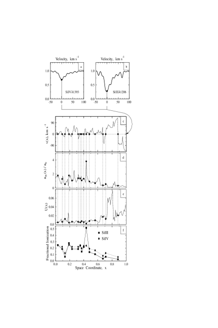
Figure 1: Velocity plots of Si iv (a) and Si iii (b) synthetic profiles calculated for the $z_{\rm a}=3.514$ system towards QSO 08279+5255 by Levshakov, Agafonova & Kegel (2000). The underlying velocity, density and ionization parameter distributions are shown in panels (c), (d), and (e), respectively. The diversity of fractional ionizations in the marked areas is illustrated in panel (f)

Having defined $n_{\rm H}(x)$, the ionization fractions $\Upsilon_{{\rm a},i}$ can be calculated using a photoionization model corresponding to that of DS or Ferland (1995). In the present paper we used the results of DS since we may neglect the radiation transfer and high-density effects incorporated in Ferland’s CLOUDY code.

2.2 Some aspects of line formation in clumpy stochastic media

When using the conventional Voigt-profile fitting (VPF) procedure several subcomponents are usually assumed to describe an absorption line which is too complex to be fitted by a single Voigt profile. Each component is supposed to represent a homogeneous plane-parallel slab of gas with its own physical parameters : radial velocity, the rms velocity, density, ionization and element abundances (see e.g. Tytler et al. 1996). This fitting method would yield physically reasonable results for gas in spatially separate homogeneous clouds if we could know a priori the actual number of these clouds and have a justification for their homogeneity. As far as the number of subcomponents is unknown, the VPF method loses uniqueness and stability. The main question remains whether the complex line shape is caused by separate homogeneous clouds or by a continuous medium with fluctuating characteristics. There are no unambiguous observational data favoring one or the other assumption. But some indirect information such as the increasing complexity of the line profiles with increasing spectral resolution and recently performed 3D hydrodynamic calculations (see e.g. Rauch, Haehnelt & Steinmetz 1997) give higher weight to the model of a fluctuating continuous medium. Applied to the inversion problem, this has important consequences.

Fig. 1 illustrates step-by-step the line formation process in a stochastic medium. The synthetic spectra of Si iv$\lambda 1393$ (panel a) and Si iii$\lambda 1206$ (panel b) are formed in an absorbing region with the fluctuating velocity and density fields shown in panels c and d, respectively. The corresponding distribution of the ionization parameter $U(x)$ is shown in panel e.

Let us consider a point within the Si iv and Si iii profiles, for example at the radial velocity $v=0$ km s^-1 (panels a and b). Then filled circles in panel c mark those volume elements having the same radial velocity. The corresponding points in panel d show the density in the corresponding areas contributing to the ‘observed’ intensity.

It is clearly seen that for a given point within the line profile the observed intensity results from a mixture of different ionization states (labeled portions of the $U$-distribution in panel e). It is also obvious that each point of the line profile is caused by a different combination of these states. As an example, panel f shows the different fractional ionizations of Si iii and Si iv at the points with $v=0$ km s^-1.

In practical applications, the metal abundances, $Z_{\rm a}$, are usually estimated from the ratio of the total column densities $N_{\rm a}$ and $N_{\rm H}$ by means of the ‘correction for the ionization’ :

$$Z_{\rm a}=\frac{N_{{\rm a},i}}{N_{{\rm H}\,{\sc i}}}\,\frac{\Upsilon_{{\rm H}\,{\sc i}}(\bar{U})}{\Upsilon_{{\rm a},i}(\bar{U})}\>.$$ (13)

The mean value of $\bar{U}$ is usually estimated from the ratio $N_{{\rm a},i}/N_{{\rm a},j}$. While this procedure is suggestive, it is incorrect if the degree of ionization varies along the line of sight. From eq. (12) and accounting for $\int\,\Phi_{\lambda}\,{\rm d}\lambda=1$, it follows that

$$\frac{N_{{\rm a},i}}{N_{{\rm a},j}}=\frac{\int\,n_{\rm H}(x)\,\Upsilon_{{\rm a},i}[U(x)]\,{\rm d}x}{\int\,n_{\rm H}(x)\,\Upsilon_{{\rm a},j}[U(x)]\,{\rm d}x}=\frac{\bar{\Upsilon}_{{\rm a},i}}{\bar{\Upsilon}_{{\rm a},j}}\>,$$ (14)

where $\bar{\Upsilon}_{{\rm a},i}$ and $\bar{\Upsilon}_{{\rm a},j}$ denote the mean density-weighted fractional ionizations.

The ratio $\Upsilon_{{\rm a},i}/\Upsilon_{{\rm a},j}$ as a function of $U$ can be calculated from the adopted photoionization model. Then the mean value of the ionization parameter, $\bar{U}$, is estimated using the implicitly assumed relation

$$\frac{\bar{\Upsilon}_{{\rm a},i}}{\bar{\Upsilon}_{{\rm a},j}}=\frac{\Upsilon_{{\rm a},i}(\bar{U})}{\Upsilon_{{\rm a},j}(\bar{U})}\>.$$ (15)

Since $\Upsilon_{{\rm a},i}$ is a non-linear function of $n_{\rm H}$, it is clear that the equality $\bar{\Upsilon}=\Upsilon(\bar{U})$ holds only in the case of a uniform density. Applying relation (15) to the case of a fluctuating gas density leads to a wrong value of $\bar{U}$ – and moreover the estimation of the mean ionization parameter will depend on the specific pair of ions chosen to calculate the left-hand side of (14).

To illustrate the numerical differences that may occur between the micro- and mesoturbulent approaches we consider the following example. The absorption lines shown in Fig. 1 have approximately the same total column densities [the data are taken from Ellison et al. 1999 ($\log N_{{\rm Si}\,{\sc iv}}\simeq 12.8$ cm^-2) and Molaro et al. 1999 ($\log N_{{\rm Si}\,{\sc iii}}\simeq 12.8$ cm^-2)]. The ratio $N_{{\rm Si}\,{\sc iii}}/N_{{\rm Si}\,{\sc iv}}\simeq 1$ suggests that $\log\bar{U}\simeq-2.2$, i.e. $\bar{U}\simeq 6.3\times 10^{-3}$. However, the mesoturbulent solution yields a 2.5 times higher value for the mean ionization parameter, i.e. $\bar{U}\simeq 1.6\times 10^{-2}$ (for more details, see Levshakov, Agafonova & Kegel 2000).

It is worthwhile to conclude this section with a few remarks concerning the VPF method. From a mathematical point of view the VPF is quite consistent since it simply means the representation of the unknown radial velocity distribution function by the sum of several Voigt functions. In such a way we can very well reproduce the line profiles and, in the case of unsaturated lines, calculate accurately the total column densities. But if we wish to go further and estimate physical parameters like kinetic temperature, ionization and metallicity, the VPF may produce misleading results. If reality corresponds to a model like that shown in Fig. 1, it is physically unjustified to interpret each subcomponent as belonging to one distinguished cloud since as shown in Fig. 1 the contribution to any point within the line profile does not come from a single separate area but from volume elements distributed over the whole absorbing region.

Figure 2: Model A, Markovian fields : the normalized velocity (a), density (b), kinetic temperature (c), and ionization parameter (d) distributions vs space coordinate ($T$ is given in units of $10^{4}$ K). The corresponding density-weighted distribution functions for the radial velocities of the gas and the individual ions are shown in panels (e) and (f). Panels (g) –(l) represent simulated spectra convolved with an instrumental profile of FWHM = 7 km s^-1 and added Gaussian noise with S/N = 50 (dots with error bars). The smooth curves show the result of the MCI fitting

3 The Monte Carlo Inversion

The Monte Carlo Inversion (MCI) of line profiles includes the estimation of the physical parameters and simultaneously of three random functions $n_{\rm H}(x)$, $T(x)$, and $v(x)$. For the equilibrium models of DS, the kinetic temperature is determined from the energy balance equation in the optically thin limit. In this case $T$ depends on the gas density only, the dependence being described approximately by a power law, i.e.

$$T\propto n_{\rm H}^{\gamma}\>,\;\;{\rm with}\;\;\gamma<0.$$ (16)

For an individual realization the remaining two random functions $n_{\rm H}(x)$ and $v(x)$ are determined as follows.

The hydrodynamic velocity and density fields are formed as a result of interference of many independent and random factors – infall and outflows, rotation, tidal flows, shock waves etc. In this case, we may consider the fluctuating amplitude of the velocity or the density along the line of sight as a kind of Brownian motion which is mathematically described by the so-called Markovian processes (e.g. Rytov et al. 1989). In particular, in case of Gaussian fields the finite difference representation of the velocity as a Markovian process has the form

$$v(x+\Delta x)=f_{\rm v}\,v(x)+\epsilon(x+\Delta x)\;,$$ (17)

where $f_{\rm v}=R_{\rm v}(\Delta x)/\sigma^{2}_{\rm v}$, $R_{\rm v}$ being the correlation between the velocity values at points separated by a distance $\Delta x$, i.e. $R_{\rm v}=\langle v(x+\Delta x)\,v(x)\rangle$, $\sigma_{\rm v}$ the velocity dispersion of bulk motions, and $\epsilon$ a random normal variable with zero mean and dispersion

$$\sigma_{\epsilon,{\rm v}}=\sigma_{\rm v}\sqrt{1-f^{2}_{\rm v}}\;.$$ (18)

The density and velocity are in general related through the continuity equation. However, since we consider one component of the velocity field only, the correlation between this component and the density is less tight and in lowest order approximation we may consider the two quantities to be statistically independent of each other.

Suppose further that the logarithmic density distribution is normal and that the dimensionless variable $y(x)=n_{\rm H}(x)/n_{0}$, with $n_{0}$ being the mean gas density has the second central moment $\sigma_{\rm y}$ characterizing the dispersion of the density field along the line of sight [this definition implies that the expectation value $E(y)=1$ for any $x$]. Then consider, by analogy with $v(x)$, a random function $\nu(x)$ with the following representation

$$\nu(x+\Delta x)=f_{\nu}\,\nu(x)+\epsilon(x+\Delta x)\;,$$ (19)

where $f_{\nu}=R_{\nu}(\Delta x)/\sigma^{2}_{\nu}$, $R_{\nu}$ being the correlation between the values of $\nu$ at points separated by a distance $\Delta x$, $\sigma_{\nu}$ the logarithmic density dispersion, and $\epsilon$ a random normal variable with zero mean and dispersion

$$\sigma_{\epsilon,\nu}=\sigma_{\nu}\sqrt{1-f^{2}_{\nu}}\;.$$ (20)

Having defined $\nu(x)$, the distribution of the hydrogen density can be obtained through Johnson’s transformation (Kendall & Stuart 1963) :

$$n_{\rm H}(x)=n_{0}\,{\rm e}^{\nu(x)-\frac{1}{2}\sigma^{2}_{\nu}}\>,$$ (21)

with the relationship between the dispersions $\sigma_{\nu}$ and $\sigma_{\rm y}$

$$\sigma_{\nu}=\sqrt{\ln(1+\sigma^{2}_{\rm y})}\>.$$ (22)

With (21), we can rewrite the expression (12) for $\tau_{{\rm a},i}(\lambda)$ in the form

$$\tau_{{\rm a},i}(\lambda)=k_{0}Z_{\rm a}N_{0}\,{\rm e}^{-\frac{1}{2}\sigma^{2}_{\nu}}$$ (23)

$$\times\int^{1}_{0}\,{\rm e}^{\nu(x)}\,\Upsilon_{{\rm a},i}[U(x)]\,\Phi_{\lambda}[\Delta\lambda_{\rm D}(x),v(x)]\,{\rm d}x.$$

where $N_{0}=n_{0}\,L$ is the expectation value of the total hydrogen column density.

Equation (23) can be simplified if we have a fully resolved profile of an optically thin line. In this case the total ion column density along the given line of sight, $N_{{\rm a},i}$, can be found directly from the observed profile (Paper II), and thus we can eliminate the unknown abundance from (23). Integrating (23) over $\lambda$ yields

$$Z_{\rm a}=\frac{N_{{\rm a},i}}{\bar{\Upsilon}_{{\rm a},i}N_{0}}\,$$ (24)

where the mean density-weighted fractional ionization $\bar{\Upsilon}_{{\rm a},i}$ is

$$\bar{\Upsilon}_{{\rm a},i}={\rm e}^{-\frac{1}{2}\sigma^{2}_{\nu}}\int^{1}_{0}\,{\rm e}^{\nu(x)}\,\Upsilon_{{\rm a},i}[U(x)]\,{\rm d}x\>.$$ (25)

Inserting (24) into (23) leads to

$$\tau_{{\rm a},i}(\lambda)\,=$$

$$\frac{k_{0}\,N_{{\rm a},i}}{\bar{\Upsilon}_{{\rm a},i}}\,{\rm e}^{-\frac{1}{2}\sigma^{2}_{\nu}}\int^{1}_{0}{\rm e}^{\nu(x)}\,\Upsilon_{{\rm a},i}[U(x)]\,\Phi_{\lambda}[\Delta\lambda_{\rm D}(x),v(x)]\,{\rm d}x\,.$$

Next, the obvious relationship

$$U(x)=\frac{n_{\rm ph}}{n_{\rm H}(x)}=\frac{MJ_{0}}{n_{0}}{\rm e}^{-\nu(x)+\frac{1}{2}\sigma^{2}_{\nu}}\>,$$ (27)

shows that the mean ionization parameter $U_{0}$ is given by the expression

$$\langle U(x)\rangle=U_{0}=\frac{MJ_{0}}{n_{0}}{\rm e}^{\sigma^{2}_{\nu}}$$ (28)

(use again the Johnson transformation to evaluate the probability density distribution of $U$). Here $M$ is a multiplicative factor introduced by DS in oder to express $n_{\rm ph}$ in terms of $J_{0}$. For the photoionizing spectrum of Mathews & Ferland, $M$ is $5.19\times 10^{15}$ (in cgs units).

Figure 3: Model B : adopted correlation function of the velocity fluctuations (dotted line) and corresponding correlation function of the density contrast fluctuations (solid line)

The result (28) has quite interesting consequences. Namely, if the density is completely homogeneous $(\sigma_{\nu}=0)$ then $U_{0}=MJ_{0}/n_{0}$. But if the density field is perturbed $(\sigma_{\nu}>0)$, then with the same mean density $n_{0}$ and the same background radiation flux $J_{0}$ one obtains a higher value of $U_{0}$ without any additional sources of ionization. Intermittent regions of low and high ionization caused by the density fluctuations may occur in this case along a given line of sight.

Now we can describe our model in detail. It is fully defined by specifying $N_{0}$ (the expectation value of the total column density), the mean value of the ionization parameter $U_{0}$, the rms values of the density and velocity fluctuations, $\sigma_{\rm y}$ and $\sigma_{\rm v}$, respectively, the correlation coefficients $f_{\nu}$ and $f_{\rm v}$, and the abundances $Z_{\rm a}$ of the elements involved in the analysis. All these parameters are components of the parameter vector $\theta$. Additionally to these physical parameters, the density and velocity distributions are to be known. The continuous random functions $v(x)$ and $\nu(x)$ are represented in our computations by their values $v_{j}$ and $\nu_{j}$ sampled at the equally spaced spatial points $x_{j}$. They are computed with the relations (17) and (19) which correlate the values at neighboring points ($j=1,2,...,{\rm k}$). To estimate $\theta$, $\{v_{j}\}^{\rm k}_{j=1}$ and $\{y_{j}\}^{\rm k}_{j=1}$ from the absorption line profiles, we have to minimize the objective function

$$\chi^{2}=\frac{1}{p}\sum^{K}_{\ell=1}\,\sum^{P_{\ell}}_{i=1}\,\left[{\cal F}^{\rm obs}_{\ell,\lambda_{i}}-{\cal F}^{\rm cal}_{\ell,\lambda_{i}}(\theta)\right]^{2}/\sigma^{2}_{\ell,i}\>.$$ (29)

Here ${\cal F}^{\rm obs}_{\ell,\lambda_{i}}$ is the observed normalized intensity of spectral line $\ell$ according to eq. (3), and $\sigma_{\ell,i}$ is the experimental error within the $i$th pixel of the line profile. ${\cal F}^{\rm cal}_{\ell,\lambda_{i}}(\theta)$ is the simulated intensity of line $\ell$ at the same $i$th pixel having wavelength $\lambda_{i}$. The total number of spectral lines involved in the optimization procedure is labeled by $K$, and the total number of data points $P=\sum^{K}_{\ell=1}\,P_{\ell}$, where $P_{\ell}$ is the number of data points for the $\ell$th line. The number of degrees of freedom is labeled by $p$.

Let us go on to consider the correlation coefficients $f_{\rm v}$ and $f_{\nu}$. As known, the Markovian processes have exponential correlation functions :  $R(\Delta x)\propto\exp(-\Delta x/l)$, where $l$ is referred to as the correlation length and depends, in general, on the spatial scale. For the step size $\Delta x/l\ll 1$, the correlation coefficient $f$ is very close to unity. The computational procedure is quite insensitive to the concrete values of $f$ because of the stochastic relations (17) and (19). Therefore the value of $f$ cannot be estimated in the same manner as other physical parameters. It appears to be more suitable to fix a few sets of $f_{\rm v}$ and $f_{\nu}$ and then to carry out the estimation of other parameters with each of these sets. Hence, in reality the parameter vector $\theta$ does not include components $f_{\rm v}$ and $f_{\nu}$.

The computational scheme is similar to that described in Paper III, but in the present work we used instead of the classical Metropolis method the more efficient generalized simulated annealing algorithm (Xiang et al. 1997).

Model calculations with different synthetic spectra have shown that the minimization of $\chi^{2}$ in form of eq. (29) does not allow us to recover the physical parameters with a sufficiently high accuracy (see also LTA). To stabilize the estimation of $\theta$, we need to augment $\chi^{2}$ by a regularization term (or a penalty function). The choice of the penalty function is rather heuristic and depends on the particular problem. For instance, when we try to fit model spectra to real noisy data it is reasonable to stop the minimization procedure at the value of $\chi^{2}\simeq 1$ in order to avoid fitting intensity fluctuations caused by the noise. Another restriction stems from the restoring procedure for the density and velocity distributions. If we use instead of the processes (17) and (19) their normalized analogies :  $v^{\ast}(x)=v(x)/\sigma_{\rm v}$ and $\nu^{\ast}(x)=\nu(x)/\sigma_{\nu}$ with the dispersions $\sigma_{{\rm v}^{\ast}}=\sigma_{\nu^{\ast}}=1$, more stable estimations for $\sigma_{\rm v}$ and $\sigma_{\nu}$ are obtained. In addition, the process $\nu^{\ast}$ should be centered, i.e. $\langle\nu^{\ast}\rangle=0$  (the center of the velocity distribution is determined by the relative positions of spectral lines and in principle can differ from zero). Accounting for all these remarks, the modified objective function is now written in the form

$${\cal L}=|\chi^{2}-1|+\alpha(|\langle\tilde{\nu}^{\ast}\rangle|+|\tilde{\sigma}_{\nu^{\ast}}-1|+|\tilde{\sigma}_{{\rm v}^{\ast}}-1|)\;,$$ (30)

where $\alpha$ is a constant of order unity and $\tilde{\nu}^{\ast}$, $\tilde{\sigma}_{\nu^{\ast}}$, $\tilde{\sigma}_{{\rm v}^{\ast}}$ are the quantities derived from the current configuration. It follows that in the vicinity of the global minimum we must have ${\cal L}_{\rm min}\approx 0$.

If the optimization of ${\cal L}$ gives $\langle v^{\ast}\rangle\neq 0$, the estimated rms velocity $\sigma_{\rm v}$ is biased. To correct its value, the following relation can be used

$$\sigma^{\rm corr}_{\rm v}=\sigma_{\rm v}\,\left(1-{\rm k}\,\langle v^{\ast}\rangle^{2}/\sum^{\rm k}_{j=1}(v^{\ast}_{j})^{2}\right)^{1/2}\;.$$ (31)

The practical implementation of the proposed computational procedure for recovering the physical parameters from spectral lines of different ions is described in the following section.

4 Numerical Experiments

Table 1: Model parameters used to generate synthetic spectra

model	$n_{0}$	$J_{0}$	$L$	$\sigma_{\rm v}$	$\sigma_{\rm y}$
	cm-3	ergs/s cm2 Hz	kpc	km/s
A	0.001	$1.5\,10^{-21}$	5.5	25	1.5
B	0.005	$3.0\,10^{-21}$	1.5	20	0.8

We tested the numerical procedure described above by inverting synthetic spectra with known physical parameters and known underlying velocity-density distributions along the line of sight. We have considered two models A and B with the physical parameters listed in Table 1.

To calculate random fields several procedures can be utilized. The most simple one has been realized in model A : the velocity and gas density fields were produced by means of two independent Markovian processes according to eqs. (17) and (19) with $f_{\rm v}=0.995$, $f_{\nu}=0.999$ and $\Delta x=1/300$. The fractional ionization for the different ions included in the analysis were then calculated using the model of DS. It is worth emphasizing that this model may not necessarily capture the physics most correctly since it assumes a specific type of the ionizing radiation, but since our purpose in this paper is to show the principal possibility of recovering the adopted physical characteristics of the absorbing region from the synthetic spectra, the DS model was chosen because of its transparency and easiness to compute. The synthetic spectra were then calculated according to eq. (12) with fixed metallicity for all ions ${\rm Z}=0.1\,{\rm Z}_{\odot}$ (solar abundances were taken from Grevesse 1984). To complete the procedure the spectra were convolved with a Gaussian point-spread function having FWHM = 7 km s^-1 and a Gaussian noise with S/N = 50 was added to each pixel (dots with error bars in Fig. 2).

Figure 4: As Fig. 2, but for model B, non-Markovian fields

Fig. 2 shows the hydrodynamic fields (normalized velocity $u=v/\sigma_{\rm v}$ and gas density) together with the kinetic temperature (in units of $10^{4}$ K) and the ionization parameter $U/U_{0}$ distributions along the line of sight (panels a – d). The histograms in panels e and f give the density-weighted velocity distributions of the different ions which determine the shapes of the spectral lines presented in turn in panels g – l for the H i Ly12, C ii, C iv, Si ii, Si iv, and O vi lines, respectively. The Ly12 line was chosen for the analysis because it is unsaturated and, hence, allows us to estimate the neutral hydrogen column density quite accurately. The choice of metallic ions was motivated by the fact that their lines are formed in different parts of the adsorbing region : C ii, for example, needs denser gas and lower temperature to be produced (the area in the vicinity of $x\simeq 0.2$), whereas O vi mainly is found in the very diffuse and hot areas ($x\simeq 0.02,0.38$ and 0.8). Such a diversity of lines in question enables us to restore the underlying density and radial velocity distributions in more detail.

Model B differs from model A not only by the values of physical parameters but by the method to generate random fields as well. To produce the stochastic velocity and density contrast, $\delta(x)$, distributions, the corresponding power spectra were utilized. The computational scheme was similar to that proposed by Bi, Ge & Fang (1995) but with another set of power spectra. We assume that the 1D power spectrum for the velocity is given and then we calculate the 1D power spectrum for $\delta$. In particular, for the normalized radial velocity distribution, $u(x)$, the following 1D power spectrum was chosen [it corresponds to the correlation function $\cal{C}$${}_{l,\varepsilon}(x)$ adopted in LTA] :

$$S^{\rm 1D}_{\rm u}(k)=\frac{k^{1-\varepsilon}\,{\rm e}^{-l\,k}}{2\,\Gamma(2-\varepsilon)l^{\varepsilon-2}}\>,$$ (32)

where $\Gamma$ is the gamma function, $l$ and $\varepsilon$ are fixed constants ($\varepsilon<2$ and $l$ is in units of $L$).

We can calculate the 1D power spectrum for the density contrast from its 3D spectrum which in turn is defined by the 3D power spectrum for the velocity : $S^{\rm 3D}_{\delta}=k^{2}\,S^{\rm 3D}_{\rm u}$. (This relation stems from the continuity equation when it is linearized in comoving coordinates). The 3D power spectrum $S^{\rm 3D}_{\rm u}$ is related to its 1D spectrum via (see Monin & Yaglom 1975) :

$$\frac{S^{\rm 1D}_{\rm u}(k)}{2\pi k^{2}}=\int^{\infty}_{k}\,\frac{S^{\rm 3D}_{\rm u}(k^{\prime})}{k^{\prime}}\,{\rm d}k^{\prime}\>,$$ (33)

and thus

$$S^{\rm 3D}_{\rm u}(k)=\frac{1}{2\pi k^{2}}\left[2\,S^{\rm 1D}_{\rm u}(k)-k\frac{{\rm d}S^{\rm 1D}_{\rm u}(k)}{{\rm d}k}\right]\>.$$ (34)

The 1D power spectrum for the density contrast is then determined directly from its 3D spectrum (Monin & Yaglom) :

$$S^{\rm 1D}_{\delta}(k)=2\pi\,\int^{\infty}_{k}\,S^{\rm 3D}_{\delta}(k^{\prime})\,k^{\prime}\,{\rm d}k^{\prime}\>.$$ (35)

Given the power spectra $S^{\rm 1D}_{\rm u}(k)$ and $S^{\rm 1D}_{\delta}(k)$, which are the Fourier transforms of the covariance functions of $u$ and $\delta$, both random fields $u(x)$ and $\delta(x)$ can be modeled using the moving-average method as described in LTA. In order to avoid the appearance of negative $n(x)$, the gas density itself is assumed to have a log-normal distribution (see e.g. Bi, Börner & Chu 1992; Bi & Davidsen 1997). It is calculated from $\delta$ according to

$$n(x)/n_{0}={\rm e}^{\delta(x)-\frac{1}{2}\langle\delta^{2}\rangle}\>.$$ (36)

The density contrast, as calculated from (36), equals $\delta(x)$ in linear approximation.

The correlation functions of the processes $u(x)$ and $\delta(x)$ with the foregoing power spectra and with the adopted parameters $\varepsilon=0.1$ and $l=0.1$ are shown in Fig. 3. They differ significantly from the exponential form corresponding to the pure Markovian process. So the objective to utilize these kind of stochastic fields was to test whether we can approximate a finite realization of an arbitrary non-Markovian process by a Markovian one. The corresponding hydrodynamic fields and line profiles for model B are shown in Fig. 4 (notations are the same as in Fig. 2).

The recovering procedure aimed at the minimization of the objective function ${\cal L}$, eq.  (30), consists of two repeating steps : firstly a random point in the physical parameter box is chosen and then the appropriate optimal velocity and density configurations are estimated. (In our actual calculations we used instead of the physical parameters $N_{0}$ and $U_{0}$ their reduced values $\hat{N}_{0}=N_{0}\,{\rm e}^{-\frac{1}{2}\sigma^{2}_{\nu}}$ and $\hat{U}_{0}=U_{0}\,{\rm e}^{-\frac{1}{2}\sigma^{2}_{\nu}}$. This was made to achieve better stability of the results).

In both steps the stochastic acceptance rule was employed. The move in the parameter space or in the velocity-density configuration space is accepted if it leads to a lower current value of ${\cal L}$. If ${\cal L}$ jumps up, then the move might be accepted according to an acceptance probability $p_{\rm a}$. Two types of the acceptance probability were used in the procedure : the standard Boltzmann-type statistics as utilized in the Metropolis algorithm

$$p_{\rm a}={\rm e}^{-\Delta{\cal L}/{\cal T}}\>,$$ (37)

and the Tsallis statistics being the generalization of the Boltzmann distribution (e.g. Xiang et al. 1997)

$$p_{\rm a}=[1-(1-q_{\rm a})\Delta{\cal L}/{\cal T}]^{1/(1-q_{\rm a})}\>,$$ (38)

where $q_{\rm a}$ is a fixed constant and ${\cal T}$ is the so-called annealing parameter (‘artificial temperature’).

Table 2: Physical parameters derived by the MCI method (rows 1-11) from the synthetic spectra shown in Fig. 4. The first and the last row lists, respectively, the adopted values (model B) and the median estimations

	$\hat{U}_{0}$	$\hat{N}_{0}$	$\sigma_{\rm v}$	$\sigma_{\rm y}$	$Z_{\rm C}$	$Z_{\rm Si}$	$Z_{\rm O}$	$\chi^{2}$	$\langle\tilde{\nu}^{\ast}\rangle$	$\tilde{\sigma}_{\nu^{\ast}}$	$\tilde{\sigma}_{{\rm v}^{\ast}}$
		cm-2	km/s
	4.426e-3	1.583e19	20.0	0.8	4.900e-5	3.550e-6	8.100e-5
1	4.392e-3	1.819e19	20.04	0.722	4.839e-5	3.488e-6	5.318e-5	1.057	-0.008	1.020	1.025
2	3.871e-3	1.744e19	22.95	0.729	4.835e-5	3.558e-6	8.409e-5	1.031	0.033	1.017	1.006
3	5.532e-3	1.580e19	24.57	1.215	4.853e-5	3.540e-6	4.516e-5	1.046	-0.028	1.009	0.937
4	3.878e-3	1.727e19	21.08	0.803	4.974e-5	3.602e-6	8.336e-5	1.095	4.0e-4	0.993	1.009
5	4.081e-3	1.837e19	21.97	0.695	4.936e-5	3.490e-6	7.794e-5	1.100	-0.013	1.005	0.986
6	3.104e-3	1.964e19	22.92	0.447	4.919e-5	3.456e-6	1.406e-4	1.095	-2.0e-4	1.012	0.966
7	5.683e-3	1.490e19	20.98	1.419	4.865e-5	3.628e-6	5.097e-5	1.103	-0.019	0.991	1.001
8	4.083e-3	1.780e19	19.56	1.206	4.988e-5	3.458e-6	7.769e-5	1.093	-0.068	0.983	1.096
9	4.520e-3	1.546e19	22.77	1.012	4.840e-5	3.701e-6	7.674e-5	1.151	-0.004	1.002	0.991
10	4.980e-3	1.630e19	26.05	0.998	4.913e-5	3.516e-6	7.615e-5	1.155	0.008	1.014	0.994
11	3.848e-3	1.821e19	20.28	0.679	4.961e-5	3.535e-6	8.471e-5	1.090	-0.013	1.000	1.017
	4.083e-3	1.727e19	21.97	0.803	4.913e-5	3.535e-6	7.674e-5

In general the acceptance after Tsallis leads to quicker convergency, but it depends strongly on the value of $q_{\rm a}$ and requires a few initial trial computations to adjust this parameter. The annealing parameter ${\cal T}$ should decrease with the simulation time to ensure the convergence to the global minimum. We used the ‘cooling’ rate of type ${\cal T}={\cal T}_{0}/(1+N_{\rm steps})^{q}$, with the initial value ${\cal T}_{0}$ and the power index $q$ having different values for both procedure steps (i.e. the move in the parameter space and the move in the density-velocity configuration space). Their values were adjusted in numerous numerical experiments with the aim to reach better stability and quicker convergency. The results presented below were obtained with ${\cal T}^{\rm par}_{0}=2.0$, ${\cal T}^{\rm d-v}_{0}=\ln\,(\chi^{2}_{0})$, $q_{\rm par}=0.5$, $q_{\rm d-v}=2$ and $q_{\rm a}=-1$ (here $\chi^{2}_{0}$ is the $\chi^{2}$ value for the initial step in the parameter space). The visiting distribution (a local search distribution providing trial values) was Gaussian in all cases with the fixed dispersion of 0.1 (in dimensionless units).

Figure 5: MCI reconstruction of the velocity and density fields for three different runs (a1,a2), (b1,b2), and (c1,c2) for model A, and (e1,e2), (f1,f2), and (g1,g2) for model B (different types of dashed and dotted lines). The adopted distributions are shown by solid lines. Panels (d) and (h) represent the corresponding density-weighted velocity distribution functions (solid line histograms are adopted distributions, whereas dashed and two types dotted lines are the MCI solutions)

The results of the computations are shown in Fig. 2 (model A, Markovian fields) and in Fig. 4 (model B, non-Markovian fields) by solid lines (panels g – l). For both cases the step size was $\Delta x=1/100$ and the correlation coefficients $f_{\rm v}=f_{\nu}=0.95$. These values were chosen as the optimal ones after several trial runs with different $\Delta x$, $f_{\rm v}$ and $f_{\nu}$.

The MCI is a probabilistic procedure. It follows that one does not know in advance if the global minimum of the objective function is reached in a single run. Several runs with different initial values should be performed to obtain the parameter estimations and their confidence levels. To illustrate the probabilistic character of the MCI solutions, Fig. 5 shows the results of three different runs for model A (left-side panels) and for model B (right-side panels). Solid lines in all panels represent adopted fields, whereas dashed and two types dotted lines are the MCI solutions. All recovered fields yield $\chi^{2}\;\raise 1.29167pt\hbox{$<$\kern-7.5pt\raise-4.73611pt\hbox{$\sim$}}\;1$, implying that the absorption spectra calculated in different runs are indistinguishable from each other. The example shown by solid lines in Fig. 2 or 4 (panels g – l) is just one of the solutions obtained for the corresponding model A or B. However, it is not possible to restore the exact pixel-to-pixel structure of the stochastic velocity and density patterns along the line of sight – many configurations are possible with equal probability. But we see that all these configurations have the same (statistically indistinguishable) density-weighted velocity distributions (panels d and h), since as already mentioned above only these distributions determine the observed line shapes. It is obvious that the quality of recovering depends crucially on the diversity of ion profiles accounted for in the MCI analysis : the more ions originating from regions with different physical conditions are considered the higher reliability of the estimated parameters can be reached.

Table 2 lists the results of 11 runs for model B (model A shows entirely analogous results). It is seen that the accuracy of the estimated parameters is rather high : the median values do not differ from the adopted ones by more than 10%. As for the confidence levels, it is obvious that much more runs are needed to calculate them with a sufficient accuracy. We have not carried out such computations since in the present context the exact values of the confidence levels are not of importance. But from the runs performed we can make some qualitative conclusions. For instance, the metallicities are estimated with very high accuracy (the error in ${\rm Z}_{\rm O}$ is explained by the weakness of the oxygen line), i.e. the numerical procedure is quite sensitive to these parameters. The dispersions of $\sigma_{\rm v}$ and $\sigma_{\rm y}$ show significantly wider margins caused by the randomness of the fields which they characterize. The estimations of $\hat{U}_{0}$ and $\hat{N}_{0}$ have an accuracy of about 20% that can be considered as quite acceptable for these physical parameters. A higher accuracy can be obtained for the estimations of the total column densities of the individual ions and for the mean (density-weighted) kinetic temperatures

$$\langle T_{{\rm a},i}\rangle=\frac{\int\,n_{{\rm a},i}(x)\,T(x)\,{\rm d}x}{\int\,n_{{\rm a},i}(x)\,{\rm d}x}\>.$$ (39)

These physical parameters are listed in Table 3 in the same order as the results presented in Table 2.

To complete this section, we note that the computational time of one run with the adopted set of the spectral lines and with two 100 components vectors representing the velocity and density random configurations takes about 10 hours on a Pentium III processor with 500 MHz.

Table 3: Physical parameters derived by the MCI method (rows 1-11) from the synthetic spectra shown in Fig. 4. The first and the last row lists, respectively, the adopted values (model B) and the median estimations

	H i	C ii	C iv	Si ii	Si iv	O vi	H i	C ii	C iv	Si ii	Si iv	O vi
	Column densities in cm-2						Mean kinetic temperatures in $10^{4}$ K
	5.92e16	5.52e13	2.76e14	4.43e12	1.80e13	6.22e12	1.75	1.74	1.88	1.74	1.84	2.16
1	5.95e16	5.24e13	2.86e14	4.33e12	1.77e13	5.14e12	1.74	1.72	1.93	1.73	1.87	2.14
2	6.07e16	5.61e13	2.65e14	4.55e12	1.75e13	5.90e12	1.74	1.72	1.89	1.73	1.84	2.14
3	5.96e16	5.52e13	2.77e14	4.45e12	1.77e13	6.05e12	1.75	1.73	1.91	1.73	1.85	2.32
4	5.85e16	5.50e13	2.79e14	4.40e12	1.79e13	5.55e12	1.74	1.72	1.89	1.73	1.85	2.14
5	6.06e16	5.68e13	2.86e14	4.43e12	1.76e13	6.64e12	1.74	1.72	1.91	1.72	1.86	2.12
6	5.98e16	5.56e13	2.82e14	4.33e12	1.78e13	6.13e12	1.74	1.73	1.87	1.74	1.84	1.97
7	5.96e16	5.51e13	2.74e14	4.53e12	1.78e13	6.30e12	1.73	1.72	1.92	1.72	1.86	2.31
8	5.96e16	5.65e13	2.87e14	4.34e12	1.77e13	6.07e12	1.75	1.74	1.89	1.74	1.85	2.21
9	5.91e16	5.47e13	2.55e14	4.61e12	1.75e13	6.48e12	1.73	1.72	1.89	1.73	1.84	2.24
10	5.97e16	5.58e13	2.79e14	4.42e13	1.76e13	8.73e12	1.74	1.73	1.90	1.73	1.85	2.26
11	5.88e16	5.55e13	2.83e14	4.37e13	1.78e13	5.98e12	1.75	1.75	1.90	1.74	1.85	2.10
	5.96e16	5.55e13	2.79e14	4.42e13	1.77e13	6.07e12	1.74	1.72	1.90	1.73	1.85	2.14

5 Conclusions

We have developed a new method to solve the inverse problem in the analysis of intergalactic (interstellar) hydrogen and metal lines arising from clumpy stochastic media. In the method, the random velocity and density configurations along the line of sight are approximated by Markovian processes. The global optimization method based upon simulated annealing is then used to fit theoretical line profiles to a set of ‘observational’ data.

The proposed procedure allows us to estimate the physical parameters of the absorbing gas such as column densities, metal abundances, mean (density-weighted) kinetic temperatures for each ion, and mean ionization parameter together with the hydrodynamic characteristics – the radial velocity dispersion and the dispersion of the density fluctuations.

The computational scheme has been tested on a variety of synthetic spectra that emulate modern observational data : the absorption lines of H i, C ii, Si ii, C iv, Si iv, and O vi which are usually observed in the Lyman limit systems ($N_{{\rm H}\,{\sc i}}\;\raise 1.29167pt\hbox{$<$\kern-7.5pt\raise-4.73611pt\hbox{$\sim$}}\;3\times 10^{17}$ cm^-2). The ionization structure of the absorbing region was calculated using the standard photoionization model of Donahue & Shull (1991) with a background ionizing spectrum given by Mathews & Ferland (1987).

The inversion procedure proved to be very effective and robust allowing us to recover the physical parameters with reasonable accuracy albeit the structure of the random velocity and density fields cannot be restored with a pixel-to-pixel conformity. However, the integral characteristics of these random fields, namely, the density-weighted velocity distribution, can be estimated quite precisely. Thus we can conclude that our procedure provides reliable results and can be applied to the analysis of real data.

Note that while performing the inversion of absorption lines, one has to take into account the following. All our computational tests have been carried out under the assumption that the spectrum of the ionizing radiation is known, i.e. we used the same Mathews & Ferland spectrum to generate ‘observational’ data and to fit them with our theoretical profiles. In reality, the characteristics of the ionizing radiation are not known exactly. Therefore in real applications several types of the background photoionizing spectra should be tried. The problem how the computational results are affected by different types of the background ionizing radiation will be studied in detail elsewhere.

The proposed method has been successfully applied to the analysis of QSO high resolution spectral data with possible deuterium absorption at $z_{\rm a}=3.514$ towards APM 08279+5255 (Levshakov, Agafonova & Kegel 2000). It has been demonstrated that the blue-side asymmetry of the hydrogen Ly$\alpha$ line can be explained quite naturally by an asymmetric configuration of the velocity field only. The results obtained revealed a considerably lower neutral hydrogen column density as compared with the VPF measurements performed by Molaro et al. (1999). In contrast to Molaro et al., we have managed to fit simultaneously all absorption lines observed in this system. These results can be considered as encouraging and favor the application of the developed computational procedure to the analysis of other high quality observational data.