The High-Ionization Nuclear Emission-Line Region of Seyfert Galaxies

Abstract

Recently Murayama & Taniguchi proposed that a significant part of the high-ionization nuclear emission-line region (HINER) in Seyfert nuclei arises from the inner wall of dusty tori because type 1 Seyfert nuclei (S1s) show the excess HINER emission with respect to type 2 Seyfert ones (S2s). This means that the radiation from the HINER has the anisotropic property and thus statistical properties of the HINER emission can be used to investigate the viewing angle toward dusty tori for various types of Seyfert nuclei. In order to investigate viewing angles toward narrow-line Seyfert 1 galaxies (NLS1s) and intermediate types of Seyferts (i.e., type 1.5, 1.8, and 1.9 Seyfert galaxies; hereafter S1.5, S1.8, and S1.9, respectively), we apply this HINER test to them. We also apply the same test for S2s with/without the hidden broad line region. A sample of Seyfert nuclei analyzed here consists of 124 Seyferts compiled from the literature.

Our main results and suggestions are as follows. (1) The NLS1s are viewed from a more face-on view toward dusty tori than the S2s. However, the HINER properties of the NLS1s are indistinguishable from those of the S1s. (2) The S1.5s appear to comprise heterogeneous populations; e.g., a) some of them may be seen from an intermediate viewing angle between S1s and S2s, b) some S1.5s are basically S1s but a significant part of the broad-line region (BLR) emission is accidentally obscured by dense, clumpy gas clouds, or c) some S1.5s are basically S2s but a part of the BLR emission can be seen from some optically-thin regions of the dusty torus. (3) The S1.8s, the S1.9s and the objects showing either a broad Pa$\beta$ line or polarized broad Balmer lines are seen from a large inclination angle and the emission from the BLRs of such objects reaches us through optically-thin parts of dusty tori. These three results support strongly the current unified model of Seyfert nuclei. And, (4) the line ratios of [Fe x]$\lambda$6374 to the low-ionization emission-lines have rather isotropic property than those of [Fe vii]$\lambda$6087. Therefore it is suggested that the [Fe x]$\lambda$6374 emission is not useful investigating the viewing angle toward the dusty torus in Seyfert nuclei. The most plausible reason seems that the [Fe x]$\lambda$6374 emission is spatially extended and thus its strength tends to show less viewing angle dependence.

1. INTRODUCTION

Seyfert galaxies have been broadly classified into two classes based on the presence or absence of broad emission lines in their optical spectra (Khachikian & Weedman 1974): Seyfert galaxies with broad lines are type 1 (hereafter S1) while those without broad lines are type 2 (S2). According to the current unified model of Seyfert nuclei (Antonucci & Miller 1985; see for a review Antonucci 1993), this difference between S1 and S2 can be explained as follows. The broad-line region (BLR) is located in the very inner region (e.g., a typical radial distance from the central black hole is $r\sim$ 0.01 pc; e.g., Peterson 1993) and is surrounded by a geometrically and optically thick dusty torus. Therefore, the visibility of the central engine as well as the BLR is strongly affected by the viewing angle toward the dusty torus and then the difference between S1s and S2s is naturally understood. Indeed, this unified scheme has been supported by various observational results, for example, obscured X-ray emission in S2s (Awaki et al. 1991; Rush et al. 1996), colors of mid-infrared (MIR) emission (Pier & Krolik 1992, 1993; Murayama, Mouri, & Taniguchi 2000), MIR luminosity distributions (Heckman, Chambers, & Postman 1992; Maiolino et al. 1995), polarized broad emission lines mentioned below, and the results of multi wavelength observational tests (Mulchaey et al. 1994). In order to understand Seyfert nuclei and active galactic nuclei (AGNs) more comprehensively, any new observational tests toward the unified model are very important.

In addition to the traditional two types of Seyfert nuclei, it is known that some Seyfert nuclei show intermediate properties between S1 and S2; type 1.2 (S1.2), type 1.5 (S1.5), type 1.8 (S1.8), and type 1.9 (S1.9) (Osterbrock & Koski 1976; Osterbrock 1977, 1981b; Cohen 1983; Winkler 1992; Whittle 1992), which show both the narrow and broad components in the Balmer emission lines. It is also noted that the objects without BLR in their optical spectra (i.e., S2s) do not comprise a simple population. First, some S2s show a broad Pa$\beta$ line (Goodrich, Veilleux, & Hill 1994; Hill, Goodrich, & Depoy 1996; Veilleux, Goodrich, & Hill 1997), providing evidence for highly reddened BLRs in these objects. Second, the hidden BLR is detected only in a part ($\sim$ 20%) of S2s in the polarized optical spectra (Antonucci & Miller 1985; Miller & Goodrich 1990; Tran, Miller, & Kay 1992; Kay 1994; Tran 1995a, 1995b, 1995c); the survey promoted by Lick Observatory found 10 S2s with the hidden broad line among 50 S2s.

Another important type of Seyfert nuclei is narrow-line Seyfert 1 galaxies (NLS1s; Davidson & Kinman 1978). Optical emission-line properties of the NLS1s are summarized as follows (e.g., Osterbrock & Pogge 1985). (1) The Balmer lines are only slightly broader than the forbidden lines such as [O iii]$\lambda$5007 (typically less than 2000 km s^-1). This property makes NLS1s a distinct type of S1s. (2) The [O iii]$\lambda$5007/H$\beta$ intensity ratio is smaller than 3. This criterion has introduced to discriminate S1s from S2s by Shuder & Osterbrock (1981). (3) They present strong Fe ii emission lines which are often seen in S1s but generally not in S2s. And, (4) the soft X-ray spectra of NLS1s are very steep (Puchnarewicz et al. 1992; Boller, Brandt, & Fink 1996; Wang, Brinkmann, & Bergeron 1996) and highly variable (Boller et al. 1996; Turner et al. 1999a). Because of these complex properties, it has not yet been fully understood what NLS1s are in the context of the current unified model of Seyfert nuclei while various models for NLS1s have been proposed (see for reviews Boller et al. 1996; Taniguchi, Murayama, & Nagao 1999).

Recently, Murayama & Taniguchi (1998a; hereafter MT98a) have found that S1s have excess [Fe vii]$\lambda$6087 emission with respect to S2s. This means that a significantly large fraction of the high-ionization nuclear emission-line region (HINER; Binette 1985; Murayama, Taniguchi, & Iwasawa 1998) traced by [Fe vii]$\lambda$6087 resides in a viewing-angle dependent region; i.e., the inner wall of dusty tori (Murayama & Taniguchi 1998b; see also Pier & Voit 1995). Accordingly, it turns out that the HINER provides the indicator of the viewing angle for dusty tori of Seyfert nuclei. In this paper, we report on our statistical analysis of the HINER in the various types of Seyfert nuclei.

2. DATA

2.1. Classification of Seyfert Nuclei

As mentioned in Section 1, there are a number of sub-types of Seyfert nuclei. Summarizing their definitions and properties, we broadly re-classify all the objects in the following way (see Table 1). 1) The type of S1.2 is included in the type of S1. These Seyferts together with typical S1s are abbreviated as BLS1s (broad-line type 1 Seyferts) because there is another type of S1s; i.e., NLS1s. 2) The type of S1.5 is kept as a distinct type because Seyfert galaxies belonging to this type are more numerous than those of the other intermediate-type Seyferts. 3) The types of S1.8 and S1.9 are basically included into the type of S2. The BLRs in these galaxies are reddened more seriously than those in both BLS1s and S1.5s. In this respect, S2s with the BLR detected only in their infrared spectra (e.g., broad Pa$\beta$ emission; hereafter S2_NIR-BLR) share the same BLR properties. Therefore, we refer these types of Seyferts as type 2 Seyferts with the reddened BLR (S2_RBLR). 4) Another important type of S2s is S2s with the hidden BLR which is detected in optical polarized spectra. In this paper, we refer this type as S2_HBLR. 5) S2s either with the reddened BLR or with the hidden BLR are also referred as S2⁺; i.e., S2⁺ = S2_RBLR + S2_HBLR. 6) In contrast, S2s without any evidence for the BLR are referred as S2^- following Taniguchi & Anabuki (1999). And, 7) both types of S2⁺ and S2^- are referred as S2_total when necessary; i.e., S2_total = S2⁺ + S2^-. Our classification scheme is summarized in Table 1.

In some cases, the classification is assigned differently to a certain Seyfert nucleus among the literature. Therefore, in Table 2, we compare the types of our sample objects with those given in some previous papers (Dahari & De Robertis 1988a; Stephens 1989; Whittle 1992; Cruz-González et al. 1994; Véron-Cetty & Véron 1998). The type adopted in this paper for each galaxy is given in the last column of Table 2. The objects classified as NLS1s in the previous literature (Osterbrock & Pogge 1985; Stephens 1989; Boller et al. 1996; Véron-Cetty & Véron 1998; Vaughan et al. 1999) are categorized as NLS1.

2.2. Data

In order to investigate HINER properties of various types of Seyfert galaxies, we are interested in the following high-ionization emission lines; [Fe vii]$\lambda$6087, [Fe x]$\lambda$6374, and [Fe xi]$\lambda$7892. In addition to these lines, we are also interested in the following low-ionization emission lines; [O iii]$\lambda$5007, [S ii]$\lambda\lambda$6717,6731, and [O i]$\lambda$6300, because of the comparison with the high-ionization emission lines. These lines are simply referred as [Fe vii], [Fe x], [Fe xi], [O iii], [O i], and [S ii], respectively. Here we should mention that some fraction of the [O iii] emission arises from the inner wall of dusty tori (Pier & Voit 1995; Murayama & Taniguchi 1998b). Therefore, it seems better to use more low-ionization emission lines such as [O i] or [S ii] as a normalization emission line. This is the reason why we have compiled the data of not only [O iii] but also [O i] and [S ii]. Though [N ii]$\lambda$6583 is also one of important low-ionization emission lines, we do not use this line because the deblending [N ii] from H$\alpha$ may not be well done if the spectral resolution is not so high. We have compiled the emission line data from the literature (Table 3) which are spectroscopic studies at wavelengths covering the emission lines of our interests. The number of compiled objects is 227; i.e., 31 NLS1s, 58 S1s, 67 S1.5s, 31 S2⁺s, and 40 S2^-s.

The detection rates of [Fe vii], [Fe x], and [Fe xi] in the sample are given in Table 4. The fraction of objects with at least one of these high-ionization lines detected are also given. This table shows that the detection rate for the S2⁺ (83.9 %) is higher than those for the other types (38.7 % $\sim$ 64.2 %). Although the reason for this fact is not clear, it may be partly because the average redshift of the S2⁺s is smaller than those of the other types (see section 2.3.1) and accordingly those objects might be observed with higher S/N. Here we mention that we do not use any upper limit data in our study.

We choose the objects which show [Fe vii] and/or [Fe x] from the sample, and consequently, the object number of our sample is 124 including 9 radio-loud galaxies; i.e., 12 NLS1s, 23 BLS1s, 43 S1.5s (including 3 radio-loud galaxies), 27 S2⁺s (including 2 radio-loud galaxies), and 19 S2^-s (including 4 radio-loud galaxies). Although the sample is not a statistically complete one in any sense, the data set is the largest one for the study of HINER ever compiled.

In Table 5, the redshift, the apparent B magnitude, the absolute B magnitude, the radio flux density at the wavelength of 6 cm, the ratio of radio to optical flux density, the 60 $\mu$m luminosity, the [O iii] luminosity, and the references for the [O iii] luminosity and the emission-line flux ratios are given for each galaxy. Those magnitudes are taken from Véron-Cetty & Véron (1998), who mentioned that they had chosen the magnitudes in the smallest possible diaphragm as they were interested in the nuclei rather than in the galaxy itself. Table 3 describes the references for Table 5.

The emission-line flux ratios for each object are given in Table 6. Each ratio is the averaged value among the references. Since it is often difficult to measure the narrow Balmer component for S1s accurately, there might be the systematic error if we make reddening corrections using the Balmer decrement method (e.g., Osterbrock 1989) for all the types of Seyferts. Therefore we do not make the reddening correction for the objects in our sample. The effect of dust extinction on our result is discussed in section 3.4.

2.3. Selection Bias

Because we do not impose any selection criteria upon our sample, it is necessary to check whether or not the various samples are appropriate for our comparative study. Systematic difference of the redshift distribution, the intrinsic AGN power distribution, and the excitation degree of the narrow-line region (NLR) gas among the various Seyfert types may cause possible biases, thus we investigate these distributions.

2.3.1 Redshift

The average redshifts and 1$\sigma$ deviations for each type are 0.0351$\pm$0.0315 for the NLS1s, 0.0550$\pm$0.0450 for the BLS1s, 0.0378$\pm$0.0401 for the S1.5s, 0.0243$\pm$0.0315 for the S2⁺s, and 0.0353$\pm$0.0309 for the S2^-s. We show the histograms of the redshift in Figure 1. It is noted that the average redshifts of the S1 and the S1.5 sample are a little higher than those of the other samples. In order to investigate whether or not the frequency distributions of the redshift are statistically different among the types of Seyferts, we apply the Kolmogorov-Smirnov (KS) statistical test (Press et al. 1988). The null hypothesis is that the redshift distributions among the NLS1s, the BLS1s, the S1.5s, the S2⁺s and the S2^-s come from the same underlying population. The results are summarized in Table 7. We give the KS probabilities for the class of S2_total, which means S2⁺ and S2^- since the numbers of the S2⁺s and the S2^-s in our sample are not so large. We give two KS probabilities for each combination; the first line gives the KS probabilities for the case including the radio-loud objects while the second line gives those for the case without the radio-loud objects. The results are nearly the same for these two cases in each combination. The results of the KS test suggest that the redshifts of the S1s are systematically higher than those of the other samples.

In this paper, our main attention is addressed to the visibility of the torus HINER emission among the different Seyfert types. Since the torus HINER is located in the inner 1 pc region around the central engine, the larger average redshift of the S1s may not affect the visibility of the torus HINER. If the S1s could have intense circumnuclear star-forming regions, such emission would contribute to the line emission. However, since it is known that S1s tend to have few such circumnuclear star-forming regions (Pogge 1989; Oliva et al. 1995; Heckman et al. 1995; González Delgado et al. 1997; Hunt et al. 1997), such contamination is expected to be negligibly small. Therefore, we conclude that our later analyses are free from the redshift difference among the samples.

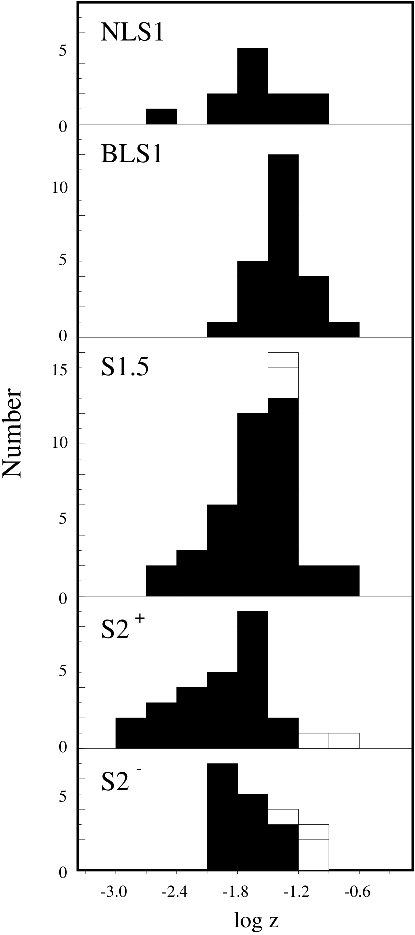
Figure 1.— Frequency distributions of the redshift among each class of Seyfert nuclei. The radio-loud galaxies are shown in white.

2.3.2 Luminosity

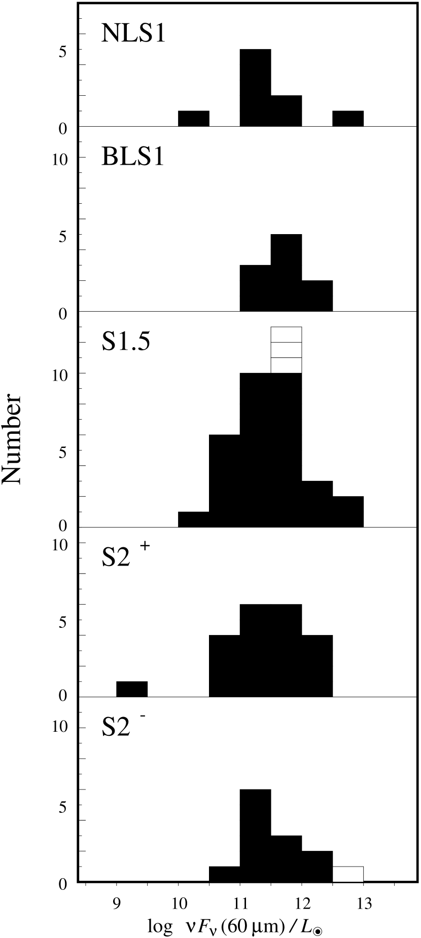
Figure 2.— Frequency distributions of the 60$\mu$m luminosity among each class of Seyfert nuclei. The radio-loud galaxies are shown in white.

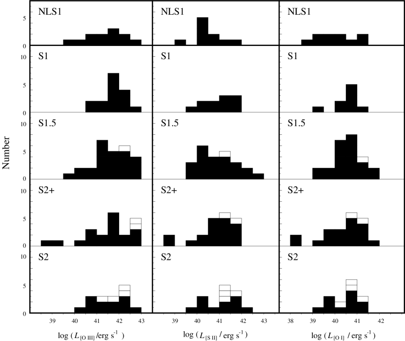
Figure 3.— Frequency distributions of the luminosities of the low-ionization emission lines among each class of Seyfert nuclei. The radio-loud galaxies are shown in white. a) The luminosity of [O iii]. b) The luminosity of [S ii]. c) The luminosity of [O i].

Current unified model of Seyfert galaxies require anisotropical nuclear radiation. This may cause systematical differences of intrinsic AGN power highly depending on selection criteria. Comparison of emission lines among different Seyfert types might suffer from this bias of intrinsic luminosity. Therefore, we investigate whether or not the intrinsic AGN power is systematically different among the different Seyfert types using the luminosities which are regarded as isotropic emission reprocessed from the nuclear radiation. We use IRAS 60$\mu$m and low-ionization emission lines as such isotropic emission.

We firstly check the distributions of the 60$\mu$m luminosity among the samples. The 60$\mu$m luminosity is thought to scale the nuclear continuum radiation which is absorbed and re-radiated by the dusty torus. Therefore the distribution of the 60$\mu$m luminosity reflects that of the intrinsic luminosity. The histograms of the 60$\mu$m luminosity are shown in Figure 2. There appears to be no systematic difference among the types of Seyferts. We apply the KS test where the null hypothesis is that the distribution of the 60$\mu$m luminosity among the various types of Seyferts come from the same underlying population. The results suggest that there is no systematic difference of the 60$\mu$m luminosity among the samples (see Table 8). This means that there is no bias concerning to the intrinsic luminosity in our sample.

However, the 60$\mu$m luminosity might be contaminated with the influence of circumnuclear star formation. Hence we secondly investigate the luminosity of the low-ionization emission lines. Because most of the flux of the low-ionization emission lines is radiated from the NLRs, it is thought to be almost independent with the viewing angle. Therefore the luminosity of a low-ionization emission line is a good tool to investigate the intrinsic power of the AGN. As shown in Figure 3, the intensity distributions of the low-ionization emission lines appear to be indistinguishable among the samples. We apply the KS test where the null hypothesis is that the luminosity of the low-ionization emission lines among various types of Seyferts come from the same underlying population. The results suggest that there is no systematic difference of the luminosity of the low-ionization emission lines among the samples (see Table 9). Therefore we conclude that there is little difference of the distribution of the intrinsic luminosity among the samples.

2.3.3 Excitation of the NLR gas

Figure 4.— The photoionization model is drown in this diagram of [S ii]/[O iii] versus [O i]/[O iii]. The calculation are performed using the spectral synthesis model CLOUDY version 90.04 (Ferland 1996). Here we assume that a uniform gas density, solar abundance, dust-free gas with plane-parallel geometry is ionized by a ‘mean Seyfert’ IR to gamma-ray continuum (with $\alpha_{\rm uv-x}$ = –1.4 in the EUV; see Ferland 1996). The free parameters for the calculations are the hydrogen density of the cloud n_H and the ionization parameter U, which is defined as the ratio of the ionizing photon density to the electron density. The values of there parameters are shown in the figure. The observed data of the NLS1s, the BLS1s, the S1.5s, the S2⁺s, and the S2^-s are shown by filled circles, open ones, triangles, diamonds, and squares, respectively.

There is another problem concerning our comparisons in this paper. In our study, we assume that the excitation degree of the NLRs is similar among the samples when we compare various line ratios. In order to confirm the validity of this assumption, we investigate whether or not the physical property of the NLRs is different among the various types of Seyferts. In Figure 4, we show the diagram of the intensity ratios of [S ii]/[O iii] versus [O i]/[O iii]. The diagram shows that there is little difference of the excitation degree of the NLRs among the types of Seyferts (see also Cohen 1983). This guarantees the validity of the statistical comparisons in our study.

3. RESULTS

Emission-line ratios of AGNs have been often discussed in the form normalized by the narrow component of Balmer lines; e.g., [O iii]/H$\beta$, [N ii]/H$\alpha$, and so on (e.g., Veilleux & Osterbrock 1987). However, since we investigate emission-line properties of S1s together with S2s, we cannot use the usual emission-line ratios in our analysis. Therefore, following the manner of MT98a, we investigate intensity ratios between a HINER line and a low-ionization forbidden emission line which is thought to be independent of the viewing-angle.

3.1. The Relative Strength of the [Fe vii] Emission

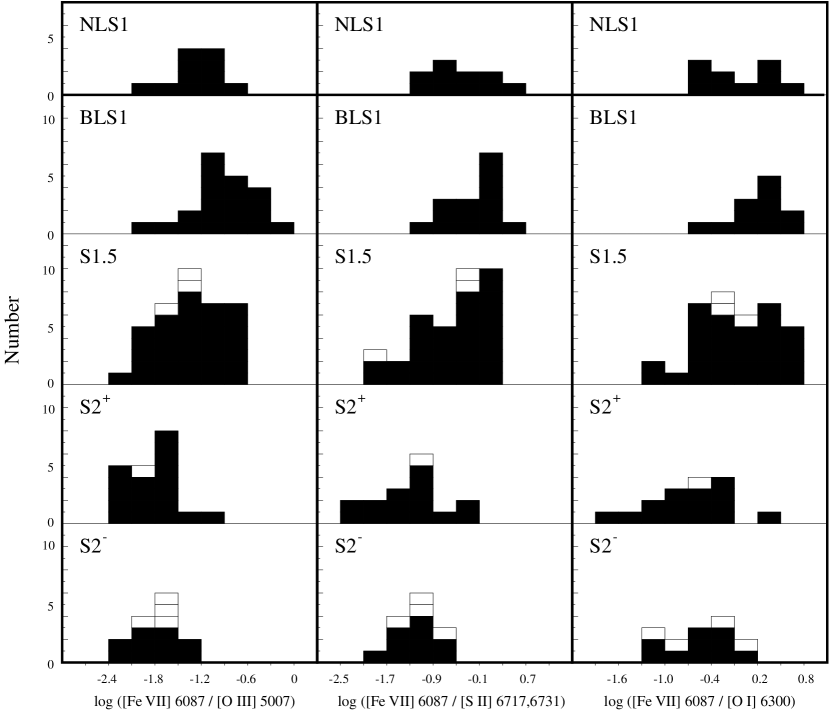
Figure 5.— Frequency distributions of the line ratio of [Fe vii] to low-ionization emission lines among the NLS1s, the BLS1s, the S1.5s, the S2⁺s, and the S2^-s. The number of radio-loud galaxies are shown in white. Left) The line ratio of [Fe vii]/[O iii]. Middle) The line ratio of [Fe vii]/[S ii]. Right) The line ratio of [Fe vii]/[O i].

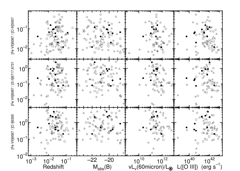
Figure 6.— Diagrams of the redshift, the absolute B magnitude, the 60$\mu$m luminosity, and the [O iii] luminosity versus the intensity ratio of [Fe vii] to low-ionization emission lines. The symbols are the same as in Figure 4. The ordinate of each diagram is the line ratio of upper) [Fe vii]/[O iii], middle) [Fe vii]/[S ii], and lower) [Fe vii]/[O i].

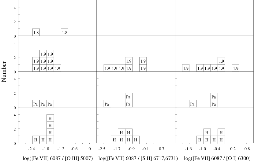
Figure 7.— Frequency distributions of the line ratio of [Fe vii] to low-ionization emission lines concerning to the S2⁺s. “1.8” means S1.8, “1.9” means S1.9, “Pa” means S2_NIR-NLR, and “H” means S2_HBLR. Left) The line ratio of [Fe vii]/[O iii]. Middle) The line ratio of [Fe vii]/[S ii]. Right) The line ratio of [Fe vii]/[O i].

We show the histograms of the line ratios of [Fe vii] to [O iii], [S ii] and [O i], for the NLS1s, the BLS1s, the S1.5s, the S2⁺s, and the S2^-s in Figure 5. Both the NLS1s and the BLS1s tend to have stronger [Fe vii] emission than the S2⁺s and the S2^-s, being consistent with the result of MT98a. It is interesting to note that the S1.5s show a marginal nature between the S1s and the S2s.

In order to investigate whether or not the differences of the emission-line ratios among the samples are statistically real, we apply the KS test. The null hypothesis is that the observed distributions of the intensity ratios of [Fe vii] to the low-ionization emission lines among the NLS1s, the BLS1s, the S1.5s, the S2⁺s and the S2^-s come from the same underlying population. The results are summarized in Table 10. It is noted that there is almost no difference between the KS probabilities in the case of including the radio-loud galaxies and excluding those objects.

The KS test leads to the following results. 1) Both the NLS1s and the BLS1s have higher [Fe vii] strengths than the S2⁺s and the S2^-s although the statistical significance is marginally low for the NLS1s when we use the [Fe vii]/[O i] ratio. 2) There is no statistical difference in the relative [Fe vii] strength between the NLS1s and the BLS1s. 3) There is no statistical difference in the relative [Fe vii] strength between the S2⁺s and the S2^-s. 4) There is no statistical difference in the relative [Fe vii] strength between the S1.5s and the S1s (i.e., the NLS1s and the BLS1s) although the statistical significance is marginally low for the BLS1s when we use the [Fe vii]/[O iii] ratio. And, 5) the S1.5s have higher [Fe vii] strengths than the S2⁺s and the S2^-s. Because the frequency distributions of the luminosity of the low-ionization emission lines are indistinguishable among the samples (see Figure 3), the excess of the line ratios of [Fe vii] to the low-ionization emission lines in both the NLS1s and the BLS1s with respect to the S2⁺s and the S2^-s is thought to be due not to the depression of the emission of the low-ionization emission lines but to the excess of the [Fe vii] emission.

It is considered that the inclination effect is responsible for the above results. In order to confirm this, we investigate whether or not the relative strength of the high-ionization emission lines correlate with the redshift or the intrinsic power of each AGN. As shown in Figure 6, there appears to be no correlation between the relative [Fe vii] strength and the redshift, the absolute B magnitude, the 60$\mu$m luminosity, and the [O iii] luminosity. Therefore the various comparisons of the emission-line flux ratios described in this paper are thought to be valid although there is slight difference in the average redshifts of the samples (see Section 2.3.1).

We also investigate the HINER properties of the S1.8s, S1.9s, S2_NIR-BLR and S2_HBLR, respectively. The results are shown in Figure 7. There can be seen no systematic trend. Therefore, these four sub-types are indistinguishable in the HINER properties.

3.2. The Relative Strength of the [Fe x] Emission

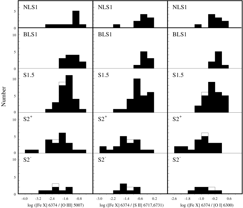
Figure 8.— Frequency distributions of the line ratio of [Fe x] to low-ionization emission lines among each class of Seyfert nuclei. The number of radio-loud galaxies are shown in white. Left) The line ratio of [Fe x]/[O iii]. Middle) The line ratio of [Fe x]/[S ii]. Right) The line ratio of [Fe x]/[S ii].

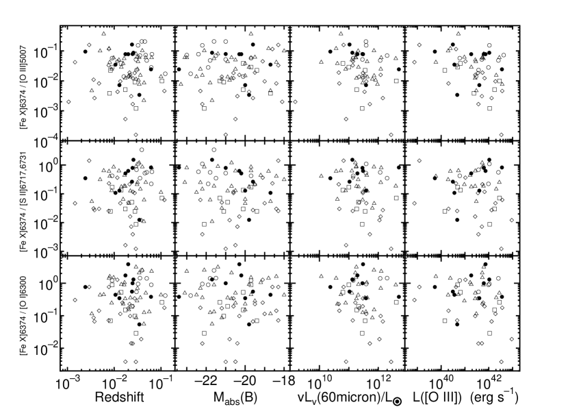
Figure 9.— Diagrams of the redshift, the absolute B magnitude, the 60$\mu$m luminosity, and the [O iii] luminosity versus the intensity ratio of [Fe x] to low-ionization emission lines. The symbols are the same as in Figure 4. The ordinate of each diagram is the line ratio of upper) [Fe x]/[O iii], middle) [Fe x]/[S ii], and lower) [Fe x]/[O i].

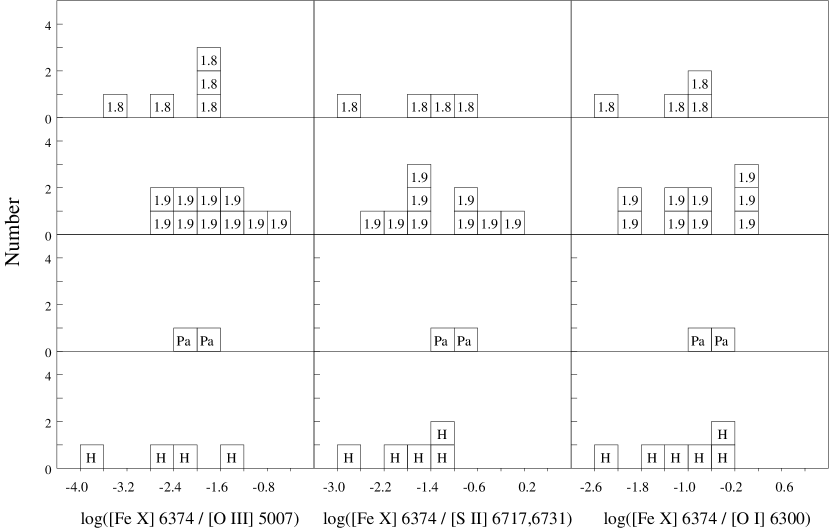
Figure 10.— Frequency distributions of the line ratio of [Fe x] to low-ionization emission lines concerning to the S2⁺s. The notations are same in Figure 7. Left) The line ratio of [Fe x]/[O iii]. Middle) The line ratio of [Fe x]/[S ii]. Right) The line ratio of [Fe x]/[O i].

We present the histograms of the intensity ratios of [Fe x] to low-ionization emission lines in Figure 8. We apply the KS test where the null hypothesis is that the observed distributions of the intensity ratios of [Fe x] to the low-ionization emission lines among various types of Seyferts come from the same underlying population. The results are given in Table 11. There is also no difference between the KS probabilities in the case of including the radio-loud galaxies and excluding those objects.

The KS test leads to the following results. 1) Both the NLS1s and the BLS1s have higher [Fe x] strengths than the S2⁺s and the S2^-s. However, the statistical significance is much worse than that using the [Fe vii] emission. 2) There is no statistical difference in the relative [Fe x] strength between the NLS1s and the BLS1s. 3) There is no statistical difference in the relative [Fe x] strength between the S2⁺s and the S2^-s 4) There is no statistical difference in the relative [Fe x] strength between the S1.5s and the S1s (i.e., the NLS1s and the BLS1s). And, 5) it is not clear whether or not there is statistical difference in the relative [Fe x] strength between the S1.5s and the S2s (i.e., S2⁺s + S2^-s). These results are not consistent with those using the [Fe vii] emission. This point will be discussed in next section.

In Figure 9, we show the diagrams of the redshift, the absolute B magnitude, the 60$\mu$m luminosity, and the [O iii] luminosity versus the relative [Fe x] strength. Similar to the case mentioned in the previous section, there is no correlation between the relative [Fe x] strength and the redshift, the absolute B magnitude, the 60$\mu$m luminosity, and the [O iii] luminosity. This result also assures the validity of our comparative study.

We also investigate the HINER properties of the S1.8s, S1.9s, S2_NIR-BLR and S2_HBLR, respectively. The result is shown in Figure 10. Again, there can be seen no systematic trend in this figure. Therefore, these four subclasses are indistinguishable in the HINER properties.

3.3. [Fe vii] versus [Fe x]

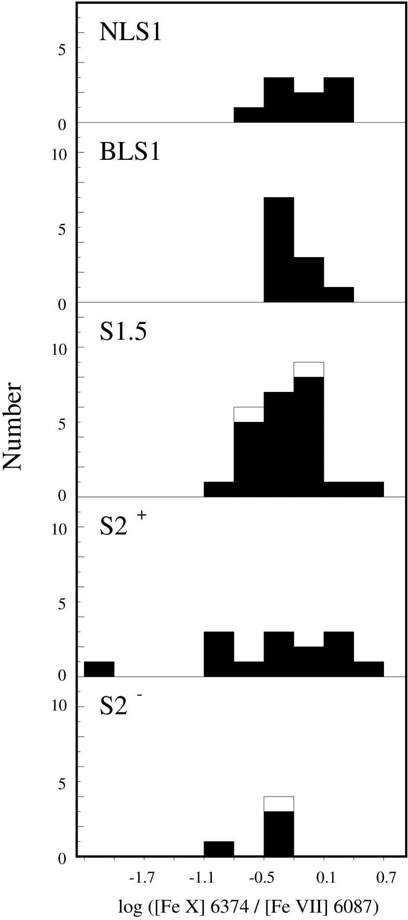
Figure 11.— Frequency distributions of the line ratio of [Fe xi] to [Fe x] among each class of Seyfert nuclei. The number of radio-loud galaxies are shown in white.

We investigate whether or not the [Fe x]/[Fe vii] ratio is different among the samples. The frequency distributions of this ratio are shown in Figure 11. We apply the KS test where the null hypothesis is that the observed distributions of the [Fe x]/[Fe vii] ratio among the various types of Seyferts come from the same underlying population. The results are given in Table 12. Although there seem to be a marginal tendency that the NLS1s have higher [Fe x]/[Fe vii] ratios than the other types of Seyferts, the KS test shows that this is not statistically real.

3.4. Effects of the Dust Extinction

As mentioned in section 2.2, no reddening correction has been made for all the observed emission line ratios analyzed here. However, it is known that the dust extinction is larger on average in S2s than in S1s (Dahari & De Robertis 1988a, 1988b). In order to see how the extinction affects the line ratios, we summarize the shifts of the line ratios for the following three cases; $A_{V}$ = 1.0, 5.2, and 10.0 (see Table 13). The case of $A_{V}$ = 5.2 corresponds to that of the Circinus galaxy (Oliva et al. 1994). In these estimates, we use the Cardelli’s extinction curve (Cardelli, Clayton, & Mathis 1989).

Since the wavelength of [O i] is relatively close to those of [Fe vii] and [Fe x], the effect of dust extinction is negligibly small even for the case of $A_{V}$ = 10.0 when the [O i] intensity is used as a normalizer. When normalized by [O iii], the effect of dust extinction leads to higher [Fe vii]/[O iii] and [Fe x]/[O iii] ratios. Because the dust extinction is larger on average in S2s than in S1s, the observational results show that these ratios are higher in the S1s than in the S2s even if the effect of the dust extinction is taken into account. On the other hand, the excess of [Fe vii]/[S ii] in both the NLS1s and the BLS1s with respect to the S2s would be extinguished if the extinction of the S2s is systematically larger (e.g., $A_{V}$ = 10) than that of the S1s. However, the average difference of the extinction between S1s and S2s is about 1 mag (Dahari & De Robertis 1988a; see also De Zotti & Gaskell 1985). Hence it is unlikely that the S2s analyzed here suffer from such larger extinction systematically. Therefore, we conclude that the results obtained in our analysis are not so seriously affected by the dust extinction.

4. DISCUSSION

4.1. The HINER in the NLS1s

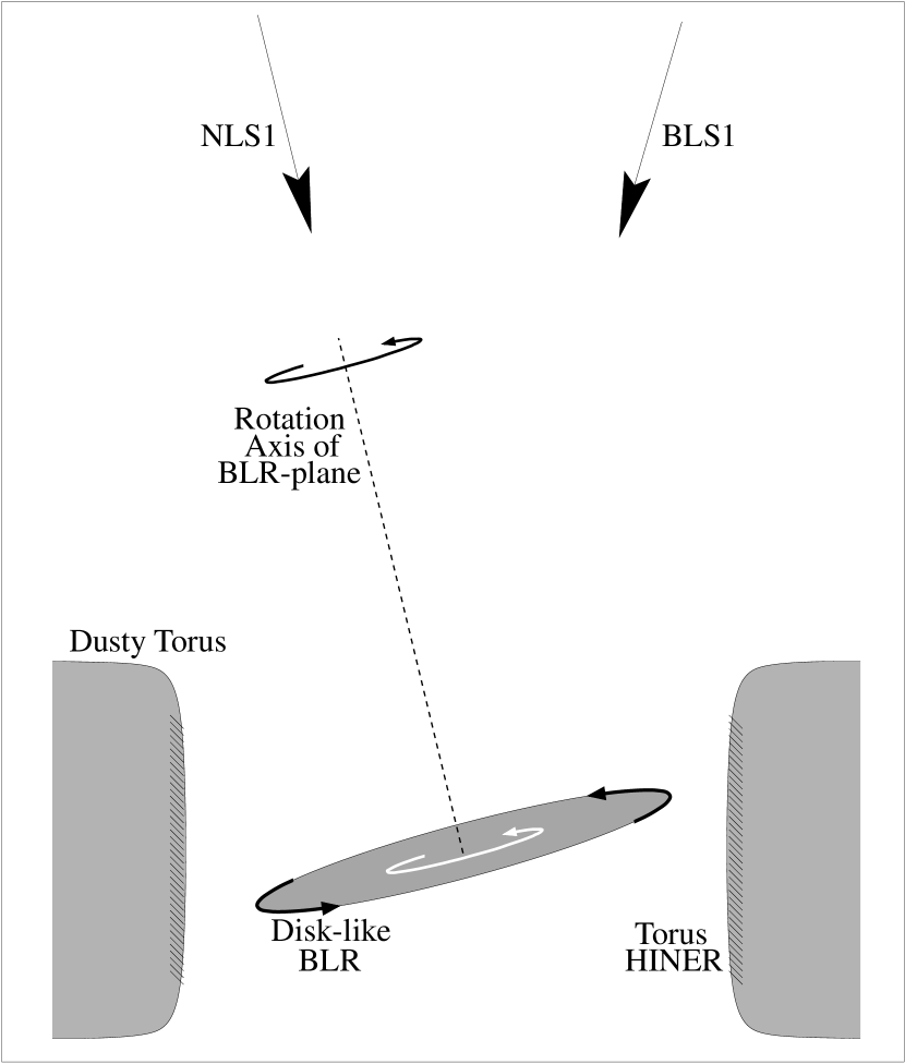
Figure 12.— A schematic illustration of the difference of the viewing angle between BLS1s and NLS1s.

Our analysis has shown that; 1) the NLS1s have higher [Fe vii] and [Fe x] strengths than the S2⁺s and the S2^-s although the statistical significance is worse when using the [Fe x] emission, and 2) there are no statistical differences in the relative strength of [Fe vii] and [Fe x] between the NLS1s and the BLS1s. Several previous works suggested that strong high-ionization emission lines are often seen in NLS1s (Davidson & Kinman 1978; Osterbrock & Pogge 1985; Nagao et al. 2000). Our analysis has statistically confirmed for the first time that the HINER emission lines of the NLS1s are significantly stronger than those of the S2s. Accordingly this suggests that the NLS1s are viewed from a more face-on view toward dusty tori than the S2s. On the other hand, the second result means that there is no systematic difference in the viewing angle toward the dusty torus between the NLS1s and the BLS1s from a statistical point of view.

Many theoretical models have been proposed to explain the properties of NLS1s (e.g., Boller et al. 1996; Taniguchi et al. 1999 and references therein). Any model is required to satisfy the statistical properties of the HINER presented in this paper; i.e., the narrow line width of NLS1s cannot be explained assuming the obscuration of broad component with dusty torus. For example, Giannuzzo & Stripe (1996) mentioned a possibility that the NLS1s may be objects seen from relatively large inclination angles and thus only outer parts of the BLR can be seen, being responsible for the narrow line width. However such models appear difficult to explain the property of HINER in the NLS1s consistently.

Since our second result means that the viewing angle toward the dusty torus is nearly the same on average between the NLS1s and the BLS1s, it is possible to propose the following model if the BLR observed in optical spectra has a disk-like configuration. Suppose that the rotational axis of the BLR is different from that of the dusty torus. In this case, the BLR line width of S1s depends on the viewing angle toward the BLR disk. However, the line width does not depend on the the viewing angle toward the dusty torus unless the BLR is not hidden by the dusty torus. This model is schematically shown in Figure 12. Our results appear consistent with this model.

It is noted that the BLR emission may arise from outer parts of a warped accretion disk (Shields 1977; Nishiura, Murayama, & Taniguchi 1998; see also for a review Osterbrock 1989). Such warping of accreting gas disks may be driven by the effect of radiation pressure force (Pringle 1996, 1997). Indeed, it has been recently shown that accreting gas clouds probed water vapor maser emission at 22 GHz show evidence for significant warping (Miyoshi et al. 1995; Begelman & Bland-Hawthorn 1997). Therefore, it is likely that the rotation axis of the BLR is not necessarily to align to that of the dusty torus.

Recently, Turner, George, & Netzer (1999b) reported on the observation of the NLS1 Akn 564. They estimated the viewing angle toward the accretion disk $\sim$60° using a model for asymmetric Fe K$\alpha$ line profile and mentioned that this result is contrary to the hypothesis that NLS1s are viewed from pole-on view. However, if the rotation axis of the accretion disk is different from those of the BLR and the dusty torus (e.g., Nishiura, Murayama, & Taniguchi 1998), their observation is not inconsistent with the HINER properties presented in this paper.

4.2. The HINER in the S1.5s

The S1.5 is widely recognized as a distinct class of Seyferts observationally (Osterbrock & Koski 1976; Cohen 1983). However, the nature of this type of Seyferts have not yet been fully understood. Comparing the HINER properties of the S1.5s with those of the other types of Seyferts, we discuss the nature of S1.5s.

Our analysis shows that; 1) there is no statistical difference in the relative [Fe vii] and [Fe x] strengths between the S1.5s and the S1s (i.e., NLS1s + BLS1s), but 2) the S1.5s have higher [Fe vii] strengths than the S2⁺s and the S2^-s although this tendency is not confirmed in the relative [Fe x] strength. In summary, as shown in Figures 5 and 8, although the S1.5s have an intermediate property in the HINER line strengths between the S1s and S2s, the relative HINER line strengths cover the whole observed ranges of both the S1s and the S2s. Therefore, there are three alternative ideas to explain these observational properties. The first idea is that the S1.5s are seen from an intermediate viewing angle between S1s and S2s; i.e., a significant part of the BLR is obscured by a dusty torus, resulting in a composite profile consisting of both the narrow-line region (NLR) and BLR emission. The second idea is that some S1.5s are basically S1s but a significant part of the BLR emission is accidentally obscured by dense, clumpy gas clouds. The third idea is that some S1.5s are basically S2s but a part of the BLR emission can be seen from some optically-thin regions of the dusty torus.

As shown in Figure 5, the majority of S1.5s has nearly the same relative [Fe vii] strengths as those of the S1s, being consistent with the second idea. The remaining minority can be explained either by the first idea or by the third one. Yet, it seems important to mention that the origin of S1.5s may be heterogeneous. Finally, it is also important to mention that the latter two ideas may explain why some Seyfert nuclei show the so-called type switching between S1 and S2; e.g., NGC 4151 (Penston & Perez 1984; Ayani & Maehara 1991). The reason for this is as follows. It seems likely that the dusty torus consists of rather small blobs which are orbiting around the central engine. When a blob is passing the line of sight to the central engine, the BLR can be obscured if the blob is optically thick enough to hide it. If we assume that the blob is located at a radial distance of 0.1 pc from the central engine and the mass of the supermassive black hole is 10⁷ M_☉, the Keplerian velocity is estimated to be V${}_{\rm rot}\sim$ 660 km s^-1. Since the typical time scale of the observed type switchings is $\sim$ 10 years, this blob could move 2 $\times$ 10¹⁶ cm. This is almost consistent with the typical size of the BLR, $\sim$ 0.01 pc (e.g., Peterson 1993). This idea also suggests that a typical size of such blobs is $\sim$ 0.01 pc.

4.3. The HINER in the “S2⁺s”

As presented in section 3, there is no statistical difference in the relative strengths of [Fe vii] and [Fe x] between S2⁺s and S2^-s . Among the subtypes of S2⁺s (i.e., S1.8, S1.9, S2_NIR-BLR and S2_HBLR), there is no systematic difference in the HINER properties (see Figures 7 and 10). On the other hand, the S2⁺s have weaker [Fe vii] strength than the S1.5s (Table 10). These facts suggest that there is a systematic difference in the viewing angle toward dusty tori between the S1.5s and the S2⁺s; i.e., the S2⁺s might be those which are seen with large inclination angle and the emission radiated from the BLR reach us through the occasionally thin dusty tori. All these arguments imply that S2⁺s are viewed from large inclination angles, leading to more significant extinction of the BLR emission with respect to BLS1s and S1.5s. This appears consistent with earlier implications (e.g., Miller & Goodrich 1990; Heisler, Lumsden, & Bailey 1997).

4.4. The Nature of HINER Traced by [Fe x]

As presented in sections 3.1 and 3.2, both the NLS1s and the BLS1s have higher HINER emission-line strengths than the S2⁺s and the S2^-s. However, comparing the KS probabilities given in Table 10 and Table 11, in particular those concerning to the relative intensities normalized by [O iii], this tendency is much more prominent in the analysis using [Fe vii] rather than [Fe x]. As proposed by MT98a, the excess [Fe vii] emission in the S1s appears attributed to the significant contribution from the torus HINER. Therefore, the weaker excess emission in [Fe x] implies that the major [Fe x] emitting region may be not the torus HINER but either the clumpy NLR HINER or the extended HINER or both because the latter two HINERs show less viewing angle dependence (see MT98a).

Another interesting property related to the [Fe x] emission is the observed [Fe x]/[Fe vii] ratios (see Figure 11). The average ratios are compared among the sample in Table 14. It is remarkable that some S1s and S2s have very higher ratios; e.g., [Fe x]/[Fe vii] $\geq$ 1. Therefore, in order to investigate the origin of the [Fe x] emission, it is interesting to compare the observed line ratios of [Fe x]/[Fe vii] with several theoretical predictions. Because simple one-zone models are known to predict too weak high-ionization emission lines (e.g., Pelat, Alloin, & Bica 1987; Dopita et al. 1997), we investigate multi-component photoionization models; 1) optically thin multi-cloud model (Ferland & Osterbrock 1986), and 2) the locally optimally emitting cloud model (LOC model; Ferguson et al. 1997). As shown in Table 14, these models predict smaller line ratios. On the other hand, the low-density interstellar matter (ISM) model by Korista & Ferland (1989) predicts higher line ratios of [Fe x]/[Fe vii]. They mentioned that such HINER will be observed out to 1 – 2 kpc. Indeed, extended HINERs have been found in some Seyfert galaxies; NGC 3516 (Golev et al. 1995), Tololo 0109$-$383 (Murayama et al. 1998), and NGC 4051 (Nagao et al. 2000). Alternatively, shock models may also be responsible for the observed higher [Fe x]/[Fe vii] ratios. Viegas-Aldrovandi & Contini (1989) calculated those ratios introducing the shock component. As shown in Table 14, such models can also explain those higher line ratios.

Which is the appropriate model for the higher line ratios of [Fe x]/[Fe vii], highly ionized low-density ISM or shock-driven ionization? In order to distinguish these two models, we compare the observed [Fe xi]/[Fe x] ratios with model results in Table 14. The [Fe xi] emission is observed in only 19 Seyfert nuclei (e.g., Grandi 1978; Cohen 1983; Penston et al. 1984; Erkens et al. 1997).As shown in Table 14, the low-density ISM models of Korista & Ferland (1989) appear consistent with the observed [Fe xi]/[Fe x]ratios. Though Viegas-Aldrovandi & Contini (1989) did not calculate this line ratio, Evans et al. (1999) mentioned that the ionization state in the emission-line region ionized by shocks is somewhat lower than that ionized by a typical nonthermal continuum. Therefore, it is likely that some Seyfert galaxies have the extended HINER described by Korista & Ferland (1989), being responsible for the unusually strong [Fe x] emission. This idea also explains why the excess [Fe x] emission is less significant in the S1s than the excess [Fe vii] emission.

5. CONCLUDING REMARKS

The anisotropic property of the radiation from the HINER traced [Fe vii] reported by MT98a has been statistically confirmed using the larger sample. The line ratios of [Fe x] to the low-ionization emission lines show a rather isotropic property with respect to those of [Fe vii] to the low-ionization emission lines. This may be interpreted by an idea that a significant fraction of the [Fe x] emission arises from low-density ISM as suggested by Korista & Ferland (1989). We note that the [Fe x] emission is not suitable to investigate the viewing angle toward the dusty tori of Seyfert nuclei.

We have also investigated the HINER properties of the intermediate-type of Seyfert nuclei. Using the frequency distributions of the line ratios of [Fe vii] to the low-ionization emission lines, we find the following suggestions. (1) The NLS1s are viewed from a more face-on orientation toward dusty tori than the S2s. (2) The line ratios of S1.5s are distributed in a wide range from the smallest value of the S2s to the largest value of the S1s. This suggests that the S1.5s are heterogeneous populations. (3) The HINER properties of the S1.8s, the S1.9s and the objects showing a broad Pa$\beta$ line or polarized broad Balmer lines are considerably different from those of the S1s. These facts mean that the “S2⁺” objects are those which are seen from a large inclination angle and their BLR emission comes through optically-thin line of sights toward the dusty tori.

Table 1Our Classification Scheme

Class	Property		Our Notations
NLS1	FWHM(H$\beta$) $<$ 2000 km s-1		NLS1
	[O iii]$\lambda$5007/H$\beta$ $<$ 3
	strong Fe ii emission
S1	showing broad Balmer lines		BLS1
S1.2	intermediate between S1 and S1.5		BLS1
S1.5	apparent narrow H$\beta$ profile superinposed on broad wings		S1.5
S1.8	intermediate between S1.5 and S2	S2RBLR	S2+	S2total
S1.9	broad component visible in H$\alpha$ but not in H$\beta$	S2RBLR	S2+	S2total
S2NIR-BLR	broad component visible in Pa$\beta$ but not in optical Balmer lines	S2RBLR	S2+	S2total
S2HBLR	broad component visible only in polarized Balmer lines		S2+	S2total
S2	broad component invisible with any method		S2-	S2total

Table 2Classification of Our Sample

Name	Another Name	DDR88	S89	W92	CG94	VCV98	This paper
Radio Quiet AGN
NGC 424	Tololo 0109-383	$\cdots$	$\cdots$	S2	$\cdots$	S1.9	S1.9
NGC 1019	$\cdots$	$\cdots$	$\cdots$	S1	S1	S1.5	S1.5
NGC 1068	M 77	S2	$\cdots$	S2	$\cdots$	S2HBLR	S2HBLR
NGC 1566	$\cdots$	S1	$\cdots$	S1.5	$\cdots$	S1.5	S1.5
NGC 2110	$\cdots$	S2	$\cdots$	S2	S2	S1.9	S1.9
NGC 2992	$\cdots$	S2	$\cdots$	S1.9	$\cdots$	S1.9	S1.9
NGC 3081	$\cdots$	S2	$\cdots$	S2	S2	S2	S2
NGC 3227	$\cdots$	S1.5	$\cdots$	S1.2	$\cdots$	S1.5	S1.5
NGC 3362	$\cdots$	$\cdots$	$\cdots$	$\cdots$	$\cdots$	S2	S2
NGC 3393	$\cdots$	$\cdots$	$\cdots$	$\cdots$	$\cdots$	S2	S2
NGC 3516	$\cdots$	S1.5	$\cdots$	S1	$\cdots$	S1.5	S1.5
NGC 3783	$\cdots$	S1	$\cdots$	S1.2	$\cdots$	S1.5	S1.5
NGC 4051	$\cdots$	S1	$\cdots$	S1.5	$\cdots$	NLS1	NLS1
NGC 4151	$\cdots$	S1.5	$\cdots$	S1.5	$\cdots$	S1.5	S1.5
NGC 4235	$\cdots$	S1.5	$\cdots$	S1.2	$\cdots$	S1.2	S1.5
NGC 4395	$\cdots$	$\cdots$	$\cdots$	$\cdots$	$\cdots$	S1.8	S1.8
NGC 4507	$\cdots$	S2	$\cdots$	S2	$\cdots$	S1.9	S1.9
NGC 4593	$\cdots$	$\cdots$	$\cdots$	S1	$\cdots$	S1	BLS1
NGC 5033	$\cdots$	S1.9	$\cdots$	$\cdots$	$\cdots$	S1.9	S1.9
NGC 5252	$\cdots$	$\cdots$	$\cdots$	S2	S2	S1.9	S1.9
NGC 5273	$\cdots$	$\cdots$	$\cdots$	S1.9	$\cdots$	S1.9	S1.9
NGC 5506	$\cdots$	S2	$\cdots$	S2	$\cdots$	S2NIR-BLR	S2NIR-BLR
NGC 5548	$\cdots$	S1.5	$\cdots$	S1.2	$\cdots$	S1.5	S1.5
NGC 5674	$\cdots$	$\cdots$	$\cdots$	$\cdots$	S2	S1.9	S1.9
NGC 5929	$\cdots$	S2	$\cdots$	S2	$\cdots$	LINER	S2
NGC 7213	$\cdots$	$\cdots$	$\cdots$	$\cdots$	$\cdots$	S1.5	S1.5
NGC 7314	$\cdots$	$\cdots$	$\cdots$	S1.9	$\cdots$	S1.9	S1.9
NGC 7469	$\cdots$	S1.5	$\cdots$	S1.2	S1	S1.5	S1.5
NGC 7674	$\cdots$	$\cdots$	$\cdots$	$\cdots$	S2	S2HBLR	S2HBLR
Mrk 1	NGC 449	S2	$\cdots$	S2	S2	S2	S2
Mrk 3	UGC 3426	S2	$\cdots$	S2	$\cdots$	S2HBLR	S2HBLR
Mrk 6	IC 450	S1.5	$\cdots$	S1.5	$\cdots$	S1.5	S1.5
Mrk 9	$\cdots$	S1	$\cdots$	S1	$\cdots$	S1.5	S1.5
Mrk 34	$\cdots$	S2	$\cdots$	S2	$\cdots$	S2	S2
Mrk 40	Arp 151	S1	$\cdots$	S1	$\cdots$	S1	BLS1
Mrk 42	$\cdots$	S1	$\cdots$	S1	$\cdots$	NLS1	NLS1
Mrk 78	$\cdots$	S2	$\cdots$	S2	$\cdots$	S2	S2
Mrk 79	UGC 3973	S1.5	$\cdots$	S1.2	$\cdots$	S1.2	S1.5
Mrk 106	$\cdots$	$\cdots$	$\cdots$	$\cdots$	$\cdots$	S1	BLS1
Mrk 110	PG 0921+525	S1	$\cdots$	S1	S1	S1.5	S1.5
Mrk 142	PG 1022+519	S1	$\cdots$	S1	$\cdots$	S1	BLS1
Mrk 176	UGC 6527	S2	$\cdots$	S2	$\cdots$	S2NIR-BLR	S2NIR-BLR
Mrk 268	$\cdots$	S2	$\cdots$	S2	$\cdots$	S2	S2
Mrk 270	NGC 5283	S2	$\cdots$	S2	$\cdots$	S2	S2
Mrk 279	UGC 8823	S1.5	$\cdots$	S1.2	$\cdots$	S1	S1.5
Mrk 290	PG 1534+580	S1.5	$\cdots$	S1	$\cdots$	S1.5	S1.5
Mrk 334	UGC 6	S1.8	$\cdots$	$\cdots$	S1.8	S1.8	S1.8
Mrk 335	PG 0003+199	S1	$\cdots$	S1	S1	S1.2	NLS1
Mrk 348	NGC 262	S2	$\cdots$	S2	S2	S2HBLR	S2HBLR
Mrk 358	$\cdots$	S1	$\cdots$	S1	$\cdots$	S1	BLS1
Mrk 359	UGC 1032	S1.5	$\cdots$	S1.5	S1	NLS1	NLS1
Mrk 374	$\cdots$	S1.5	$\cdots$	$\cdots$	$\cdots$	S1.2	S1.5
Mrk 376	$\cdots$	S1	$\cdots$	$\cdots$	$\cdots$	S1.5	S1.5
Mrk 477	I Zw 92	S2	$\cdots$	S2	$\cdots$	S2HBLR	S2HBLR
Mrk 486	PG 1535+547	S1	$\cdots$	S1	$\cdots$	S1	BLS1
Mrk 506	$\cdots$	S1.5	$\cdots$	S1.2	$\cdots$	S1.5	S1.5
Mrk 509	$\cdots$	S1.5	$\cdots$	S1.2	S1	S1.5	S1.5
Mrk 541	$\cdots$	$\cdots$	$\cdots$	$\cdots$	$\cdots$	S1	BLS1
Mrk 573	UGC 1214	S2	$\cdots$	S2	S2	S2	S2
Mrk 607	NGC 1320	S2	$\cdots$	S2	$\cdots$	S2	S2
Mrk 618	$\cdots$	S1	$\cdots$	S1	$\cdots$	S1	BLS1
Mrk 686	NGC 5695	S2	$\cdots$	$\cdots$	S2	S2	S2
Mrk 699	III Zw 77	S1	$\cdots$	S1.2	S1	S1.5	S1.5
Mrk 704	$\cdots$	S1.5	$\cdots$	S1.2	S1	S1.2	S1.5
Mrk 705	UGC 5025	S1	$\cdots$	$\cdots$	S1	S1.2	BLS1
Mrk 766	NGC 4253	S1.5	$\cdots$	S1.5	S1	S1.5	NLS1
Mrk 783	$\cdots$	S1	$\cdots$	$\cdots$	$\cdots$	NLS1	NLS1
Mrk 817	UGC 9412	S1.5	$\cdots$	S1.2	$\cdots$	S1.5	S1.5
Mrk 841	PG 1501+106	S1.5	$\cdots$	$\cdots$	$\cdots$	S1.5	S1.5
Mrk 864	$\cdots$	$\cdots$	BLS1	$\cdots$	$\cdots$	S1.5	S1.5
Mrk 871	IC 1198	S1.5	$\cdots$	S1.2	$\cdots$	S1.5	S1.5
Mrk 876	PG 1613+658	S1.5	$\cdots$	$\cdots$	$\cdots$	S1	S1.5
Mrk 926	MCG -2-58-22	S1.5	$\cdots$	S1.2	$\cdots$	S1.5	S1.5
Mrk 975	UGC 774	S1	$\cdots$	S1.2	S1	S1	BLS1
Mrk 993	UGC 987	S2	$\cdots$	$\cdots$	$\cdots$	S1.5	S1.5
Mrk 1040	NGC 931	S1.5	$\cdots$	S1.2	S1	S1	S1.5
Mrk 1126	NGC 7450	S1.5	$\cdots$	S1.5	$\cdots$	S1.5	NLS1
Mrk 1157	NGC 591	S2	$\cdots$	S2	$\cdots$	S2	S2
Mrk 1239	$\cdots$	S1	$\cdots$	S1.2	S1	NLS1	NLS1
Mrk 1388	$\cdots$	S2	$\cdots$	S2	$\cdots$	S1.9	S1.9
Mrk 1393	Tol 1506.3-00	$\cdots$	$\cdots$	$\cdots$	$\cdots$	S1.5	S1.5
1H 2107-097	H 2106-099	$\cdots$	$\cdots$	$\cdots$	$\cdots$	S1.2	BLS1
2E 1519+2754	[HB89] 1519+279	$\cdots$	BLS1	$\cdots$	$\cdots$	S1.2	S1
2E 1530+1511	[HB89] 1530+151	$\cdots$	BLS1	$\cdots$	$\cdots$	S1.2	S1
2E 1556+2725	PGC 56527	$\cdots$	BLS1	$\cdots$	$\cdots$	S1.2	S1
I Zw 1	UGC 545	S1.5	$\cdots$	$\cdots$	S1	NLS1	NLS1
II Zw 136	UGC 11763	S1	$\cdots$	S1	$\cdots$	S1.5	S1.5
Akn 120	UGC 3271	$\cdots$	$\cdots$	S1	$\cdots$	S1	BLS1
Akn 564	UGC 12163	S1	$\cdots$	S1.2	S1	NLS1	NLS1
Circinus	$\cdots$	$\cdots$	$\cdots$	$\cdots$	$\cdots$	S2HBLR	S2HBLR
ESO 141-G55	$\cdots$	$\cdots$	$\cdots$	S1	$\cdots$	S1.2	BLS1
ESO 362-G18	MCG -5-13-17	$\cdots$	$\cdots$	$\cdots$	$\cdots$	S1.5	S1.5
ESO 439-G09	Tololo 16	$\cdots$	$\cdots$	$\cdots$	$\cdots$	S2	S2
Fairall 9	$\cdots$	$\cdots$	$\cdots$	S1	$\cdots$	S1.2	BLS1
Fairall 51	ESO 140-G043	$\cdots$	$\cdots$	S1.2	$\cdots$	S1.5	S1.5
Fairall 1116	$\cdots$	$\cdots$	$\cdots$	$\cdots$	$\cdots$	S1	BLS1
IC 4329A	$\cdots$	$\cdots$	$\cdots$	S1	$\cdots$	S1.2	BLS1
KAZ320	2MASX1 J2259329+245505	$\cdots$	$\cdots$	$\cdots$	$\cdots$	NLS1	NLS1
MCG -6-30-15	ESO 383-G035	$\cdots$	$\cdots$	$\cdots$	$\cdots$	S1.5	S1.5
MCG 8-11-11	UGC 3374	S1.5	$\cdots$	S1.5	$\cdots$	S1.5	S1.5
MS 01119-0132	[HB89] 0111-015	$\cdots$	NLS1	$\cdots$	$\cdots$	NLS1	NLS1
MS 04124-0802	IRAS 04124-0803	$\cdots$	S1.5	$\cdots$	$\cdots$	S1.5	S1.5
MS 08495+0805	$\cdots$	$\cdots$	BLS1	$\cdots$	$\cdots$	S1.2	BLS1
MS 13285+3135	[HB89] 1328+315	$\cdots$	S1.5	$\cdots$	$\cdots$	S1.5	S1.5
PKS 2048-57	IC 5063	$\cdots$	$\cdots$	S2	$\cdots$	S1.9	S1.9
SBS 1318+605	$\cdots$	$\cdots$	$\cdots$	$\cdots$	$\cdots$	S1.5	S1.5
Tololo 1351-375	Tololo 113	$\cdots$	$\cdots$	S1.9	$\cdots$	S1.9	S1.9
Tololo 20	$\cdots$	$\cdots$	$\cdots$	$\cdots$	$\cdots$	$\cdots$	BLS1
Ton 1542	Akn 374	$\cdots$	$\cdots$	$\cdots$	$\cdots$	S1	BLS1
UGC 1395	$\cdots$	$\cdots$	$\cdots$	S1.8	$\cdots$	S1.9	S1.8
UGC 6100	A 1058+45	$\cdots$	$\cdots$	$\cdots$	S2	S2	S2
UGC 8621	$\cdots$	$\cdots$	$\cdots$	$\cdots$	$\cdots$	S1.8	S1.8
UGC 10683B	$\cdots$	$\cdots$	$\cdots$	$\cdots$	$\cdots$	S1.5	S1.5
UGC 12138	A 2237+07	$\cdots$	$\cdots$	$\cdots$	S1	S1.8	S1.8
Zw 0033+45	CGCG 535-012	$\cdots$	$\cdots$	$\cdots$	S1	S1.2	BLS1
Radio Loud AGN
3C 33	$\cdots$	$\cdots$	$\cdots$	$\cdots$	$\cdots$	S2	S2
3C 120	II Zw 14	$\cdots$	$\cdots$	$\cdots$	$\cdots$	S1.5	S1.5
3C 184.1	$\cdots$	$\cdots$	$\cdots$	$\cdots$	$\cdots$	S2NIR-BLR	S2NIR-BLR
3C 223	$\cdots$	$\cdots$	$\cdots$	$\cdots$	$\cdots$	S2NIR-BLR	S2NIR-BLR
3C 223.1	$\cdots$	$\cdots$	$\cdots$	$\cdots$	$\cdots$	S2	S2
3C 327	IRAS 15599+0206	$\cdots$	$\cdots$	$\cdots$	$\cdots$	S2	S2
3C 390.3	$\cdots$	$\cdots$	$\cdots$	$\cdots$	$\cdots$	S1.5	S1.5
3C 445	IRAS F22212-0221	$\cdots$	$\cdots$	$\cdots$	$\cdots$	S1.5	S1.5
3C 452	$\cdots$	$\cdots$	$\cdots$	$\cdots$	$\cdots$	S2	S2

Table 3References for Optical Emission-Lines

Abbreviation	References
C77	Costero & Osterbrock (1977)
C81	Cohen & Osterbrock (1981)
C83	Cohen (1983)
C91	Crenshaw, Peterson, Korista, Wagner, & Aufdenberg (1991)
C94	Cruz-Gonzalez, Carrasco, Serrano, Guichard, Dultzin-Hacyan, & Bisiacchi (1994)
D78	Davidson & Kinman (1978)
D86	De Robertis & Osterbrock (1986)
D88	Diaz, Prieto, & Wamsteker (1988)
E97	Erkens, Wagner, & Appenzeller (1997)
E99	Erkens, Wagner, & Appenzeller, private communication (1999)
F83	Fosbury & Sansom (1983)
K78	Koski (1978)
K79	Kunth & Sargent (1979)
K94	Kraemer, Wu, Crenshaw, & Harrington (1994)
M88	Morris & Ward (1988)
M94	Martel & Osterbrock (1994)
M95	Murayama (1995)
M98	Murayama, Taniguchi, & Iwasawa (1998)
O77	Osterbrock (1977)
O78	O’Connell & Kingham (1978)
O81	Osterbrock (1981a)
O85	Osterbrock (1985)
O93	Osterbrock & Martel (1993)
O94	Oliva, Salvati, Moorwood, & Marconi (1994)
OP	Osterbrock & Pogge (1985)
P78	Phillips (1978)
P84	Penston, Fosbury, Boksenberg, Ward, & Wilson (1984)
R97	Reynolds, Ward, Fabian, & Celotti (1997)
S80	Shuder (1980)
S89	Stephens (1989)
V88	Veilleux (1988)
W92	Winkler (1992)
Z92	Zamorano, Gallego, Rego, Vitores, & Gonzalez-Riestra (1992)

Table 4The Detection Rates of the High-Ionization Emission Lines

Class	[Fe VII]$\lambda$6087	[Fe X]$\lambda$6374	[Fe XI]$\lambda$7892	In Total
NLS1	11/30	10/29	5/8	12/31 (38.7%)
BLS1	21/58	13/52	5/19	24/58 (41.4%)
S1.5	38/67	31/62	8/30	43/67 (64.2%)
S2+	19/31	23/29	2/9	26/31 (83.9%)
S2-	15/39	9/35	2/7	19/40 (47.5%)

Table 7The Results of the KS Test Concerning the Redshift

Class	NLS1	BLS1	S1.5	S2total	S2+	S2-
NLS1	$\cdots$	1.264$\times$10-2	5.466$\times$10-1	4.200$\times$10-1	3.539$\times$10-1	8.035$\times$10-1
	$\cdots$	1.264$\times$10-2	7.243$\times$10-1	1.641$\times$10-1	2.182$\times$10-1	3.146$\times$10-1
BLS1	$\cdots$	$\cdots$	4.103$\times$10-2	5.227$\times$10-5	8.097$\times$10-6	3.972$\times$10-2
	$\cdots$	$\cdots$	2.631$\times$10-2	1.104$\times$10-6	9.773$\times$10-7	2.183$\times$10-3
S1.5	$\cdots$	$\cdots$	$\cdots$	1.568$\times$10-2	2.502$\times$10-3	6.824$\times$10-1
	$\cdots$	$\cdots$	$\cdots$	2.182$\times$10-3	1.325$\times$10-3	1.603$\times$10-1
S2total	$\cdots$	$\cdots$	$\cdots$	$\cdots$	$\cdots$	$\cdots$
	$\cdots$	$\cdots$	$\cdots$	$\cdots$	$\cdots$	$\cdots$
S2+	$\cdots$	$\cdots$	$\cdots$	$\cdots$	$\cdots$	1.330$\times$10-1
	$\cdots$	$\cdots$	$\cdots$	$\cdots$	$\cdots$	1.366$\times$10-1
S2-	$\cdots$	$\cdots$	$\cdots$	$\cdots$	$\cdots$	$\cdots$
	$\cdots$	$\cdots$	$\cdots$	$\cdots$	$\cdots$	$\cdots$

Table 8The Results of the KS Test Concerning the 60$\mu$m Luminosities of Our Sample

Class	NLS1s	BLS1s	S1.5s	S2totals	S2+s	S2-s
NLS1s	$\cdots$	4.494$\times$10-1	7.662$\times$10-1	9.992$\times$10-1	9.937$\times$10-1	9.427$\times$10-1
	$\cdots$	4.494$\times$10-1	8.571$\times$10-1	9.998$\times$10-1	9.937$\times$10-1	9.783$\times$10-1
BLS1s	$\cdots$	$\cdots$	2.175$\times$10-1	1.260$\times$10-1	2.294$\times$10-1	1.661$\times$10-1
	$\cdots$	$\cdots$	1.306$\times$10-1	1.037$\times$10-1	2.294$\times$10-1	1.072$\times$10-1
S1.5s	$\cdots$	$\cdots$	$\cdots$	7.097$\times$10-1	7.969$\times$10-1	7.049$\times$10-1
	$\cdots$	$\cdots$	$\cdots$	7.304$\times$10-1	9.088$\times$10-1	6.348$\times$10-1
S2totals	$\cdots$	$\cdots$	$\cdots$	$\cdots$	$\cdots$	$\cdots$
	$\cdots$	$\cdots$	$\cdots$	$\cdots$	$\cdots$	$\cdots$
S2+s	$\cdots$	$\cdots$	$\cdots$	$\cdots$	$\cdots$	5.086$\times$10-1
	$\cdots$	$\cdots$	$\cdots$	$\cdots$	$\cdots$	6.010$\times$10-1
S2-s	$\cdots$	$\cdots$	$\cdots$	$\cdots$	$\cdots$	$\cdots$
	$\cdots$	$\cdots$	$\cdots$	$\cdots$	$\cdots$	$\cdots$

Table 9The Results of the KS Test Concirning the Luminosities of the Low-Ionization Emission Lines

Class	NLS1	BLS1	S1.5	S2total	S2+	S2-
L${}_{\rm[OIII]}\lambda$5007
NLS1	$\cdots$	5.263$\times$10-1	7.513$\times$10-1	8.837$\times$10-1	9.158$\times$10-1	6.220$\times$10-1
	$\cdots$	5.263$\times$10-1	7.779$\times$10-1	9.919$\times$10-1	9.9999$\times$10-1	7.864$\times$10-1
BLS1	$\cdots$	$\cdots$	5.188$\times$10-1	6.077$\times$10-1	6.827$\times$10-1	6.325$\times$10-1
	$\cdots$	$\cdots$	5.805$\times$10-1	3.852$\times$10-1	4.535$\times$10-1	4.370$\times$10-1
S1.5	$\cdots$	$\cdots$	$\cdots$	9.636$\times$10-1	8.272$\times$10-1	9.020$\times$10-1
	$\cdots$	$\cdots$	$\cdots$	7.769$\times$10-1	7.200$\times$10-1	8.878$\times$10-1
S2total	$\cdots$	$\cdots$	$\cdots$	$\cdots$	$\cdots$	$\cdots$
	$\cdots$	$\cdots$	$\cdots$	$\cdots$	$\cdots$	$\cdots$
S2+	$\cdots$	$\cdots$	$\cdots$	$\cdots$	$\cdots$	9.160$\times$10-1
	$\cdots$	$\cdots$	$\cdots$	$\cdots$	$\cdots$	9.524$\times$10-1
S2-	$\cdots$	$\cdots$	$\cdots$	$\cdots$	$\cdots$	$\cdots$
	$\cdots$	$\cdots$	$\cdots$	$\cdots$	$\cdots$	$\cdots$
L${}_{\rm[SII]}\lambda\lambda$6717,6731
NLS1	$\cdots$	1.822$\times$10-1	2.596$\times$10-1	5.309$\times$10-2	1.283$\times$10-1	6.558$\times$10-2
	$\cdots$	1.822$\times$10-1	3.425$\times$10-1	2.086$\times$10-1	2.108$\times$10-1	4.339$\times$10-1
BLS1	$\cdots$	$\cdots$	6.666$\times$10-1	9.452$\times$10-1	9.892$\times$10-1	9.495$\times$10-1
	$\cdots$	$\cdots$	6.214$\times$10-1	9.747$\times$10-1	9.855$\times$10-1	9.852$\times$10-1
S1.5	$\cdots$	$\cdots$	$\cdots$	7.806$\times$10-1	8.857$\times$10-1	6.350$\times$10-1
	$\cdots$	$\cdots$	$\cdots$	8.581$\times$10-1	8.800$\times$10-1	9.830$\times$10-1
S2total	$\cdots$	$\cdots$	$\cdots$	$\cdots$	$\cdots$	$\cdots$
	$\cdots$	$\cdots$	$\cdots$	$\cdots$	$\cdots$	$\cdots$
S2+	$\cdots$	$\cdots$	$\cdots$	$\cdots$	$\cdots$	9.889$\times$10-1
	$\cdots$	$\cdots$	$\cdots$	$\cdots$	$\cdots$	9.897$\times$10-1
S2-	$\cdots$	$\cdots$	$\cdots$	$\cdots$	$\cdots$	$\cdots$
	$\cdots$	$\cdots$	$\cdots$	$\cdots$	$\cdots$	$\cdots$
L${}_{\rm[OI]}\lambda$6300
NLS1	$\cdots$	4.384$\times$10-1	3.608$\times$10-2	1.316$\times$10-1	2.555$\times$10-1	1.535$\times$10-1
	$\cdots$	4.384$\times$10-1	4.299$\times$10-2	3.079$\times$10-1	3.889$\times$10-1	5.019$\times$10-1
BLS1	$\cdots$	$\cdots$	8.700$\times$10-1	9.197$\times$10-1	8.719$\times$10-1	8.361$\times$10-1
	$\cdots$	$\cdots$	8.034$\times$10-1	6.882$\times$10-1	7.471$\times$10-1	8.581$\times$10-1
S1.5	$\cdots$	$\cdots$	$\cdots$	7.326$\times$10-1	9.343$\times$10-1	8.019$\times$10-1
	$\cdots$	$\cdots$	$\cdots$	6.632$\times$10-1	9.268$\times$10-1	6.851$\times$10-1
S2total	$\cdots$	$\cdots$	$\cdots$	$\cdots$	$\cdots$	$\cdots$
	$\cdots$	$\cdots$	$\cdots$	$\cdots$	$\cdots$	$\cdots$
S2+	$\cdots$	$\cdots$	$\cdots$	$\cdots$	$\cdots$	9.379$\times$10-1
	$\cdots$	$\cdots$	$\cdots$	$\cdots$	$\cdots$	9.665$\times$10-1
S2-	$\cdots$	$\cdots$	$\cdots$	$\cdots$	$\cdots$	$\cdots$
	$\cdots$	$\cdots$	$\cdots$	$\cdots$	$\cdots$	$\cdots$

Table 10The Results of the KS Test Concerning [Fe vii]

Class	NLS1	BLS1	S1.5	S2total	S2+	S2-
[Fe vii]$\lambda$6087 / [O iii]$\lambda$5007
NLS1	$\cdots$	7.954$\times$10-2	3.460$\times$10-1	1.050$\times$10-4	5.309$\times$10-4	8.114$\times$10-4
	$\cdots$	7.954$\times$10-2	5.626$\times$10-1	2.253$\times$10-4	6.874$\times$10-4	3.954$\times$10-3
BLS1	$\cdots$	$\cdots$	2.150$\times$10-3	1.387$\times$10-8	9.316$\times$10-7	2.190$\times$10-6
	$\cdots$	$\cdots$	5.622$\times$10-3	8.041$\times$10-8	1.609$\times$10-6	2.644$\times$10-5
S1.5	$\cdots$	$\cdots$	$\cdots$	5.093$\times$10-6	1.350$\times$10-5	9.136$\times$10-4
	$\cdots$	$\cdots$	$\cdots$	1.805$\times$10-5	2.375$\times$10-4	2.417$\times$10-3
S2total	$\cdots$	$\cdots$	$\cdots$	$\cdots$	$\cdots$	$\cdots$
	$\cdots$	$\cdots$	$\cdots$	$\cdots$	$\cdots$	$\cdots$
S2+	$\cdots$	$\cdots$	$\cdots$	$\cdots$	$\cdots$	5.090$\times$10-1
	$\cdots$	$\cdots$	$\cdots$	$\cdots$	$\cdots$	9.630$\times$10-1
S2-	$\cdots$	$\cdots$	$\cdots$	$\cdots$	$\cdots$	$\cdots$
	$\cdots$	$\cdots$	$\cdots$	$\cdots$	$\cdots$	$\cdots$
[Fe vii]$\lambda$6087 / [S ii]$\lambda\lambda$6717,6731
NLS1	$\cdots$	1.355$\times$10-1	9.684$\times$10-1	5.305$\times$10-4	3.406$\times$10-3	1.699$\times$10-3
	$\cdots$	1.355$\times$10-1	9.756$\times$10-1	1.191$\times$10-3	4.596$\times$10-3	6.899$\times$10-3
BLS1	$\cdots$	$\cdots$	1.388$\times$10-1	4.616$\times$10-7	2.248$\times$10-5	1.130$\times$10-5
	$\cdots$	$\cdots$	1.930$\times$10-1	2.468$\times$10-6	4.265$\times$10-5	1.507$\times$10-4
S1.5	$\cdots$	$\cdots$	$\cdots$	7.373$\times$10-5	3.320$\times$10-3	1.586$\times$10-3
	$\cdots$	$\cdots$	$\cdots$	5.509$\times$10-4	6.479$\times$10-3	9.612$\times$10-3
S2total	$\cdots$	$\cdots$	$\cdots$	$\cdots$	$\cdots$	$\cdots$
	$\cdots$	$\cdots$	$\cdots$	$\cdots$	$\cdots$	$\cdots$
S2+	$\cdots$	$\cdots$	$\cdots$	$\cdots$	$\cdots$	9.302$\times$10-1
	$\cdots$	$\cdots$	$\cdots$	$\cdots$	$\cdots$	9.474$\times$10-1
S2-	$\cdots$	$\cdots$	$\cdots$	$\cdots$	$\cdots$	$\cdots$
	$\cdots$	$\cdots$	$\cdots$	$\cdots$	$\cdots$	$\cdots$
[Fe vii]$\lambda$6087 / [O i]$\lambda$6300
NLS1	$\cdots$	1.902$\times$10-1	9.684$\times$10-1	2.995$\times$10-2	1.958$\times$10-2	1.036$\times$10-1
	$\cdots$	1.902$\times$10-1	9.972$\times$10-1	3.608$\times$10-2	2.481$\times$10-2	1.108$\times$10-1
BLS1	$\cdots$	$\cdots$	6.286$\times$10-2	6.120$\times$10-6	2.519$\times$10-5	3.125$\times$10-4
	$\cdots$	$\cdots$	8.606$\times$10-2	6.405$\times$10-6	3.748$\times$10-5	4.708$\times$10-4
S1.5	$\cdots$	$\cdots$	$\cdots$	9.470$\times$10-4	1.631$\times$10-3	3.159$\times$10-2
	$\cdots$	$\cdots$	$\cdots$	2.561$\times$10-3	5.638$\times$10-3	6.327$\times$10-2
S2total	$\cdots$	$\cdots$	$\cdots$	$\cdots$	$\cdots$	$\cdots$
	$\cdots$	$\cdots$	$\cdots$	$\cdots$	$\cdots$	$\cdots$
S2+	$\cdots$	$\cdots$	$\cdots$	$\cdots$	$\cdots$	7.579$\times$10-1
	$\cdots$	$\cdots$	$\cdots$	$\cdots$	$\cdots$	7.159$\times$10-1
S2-	$\cdots$	$\cdots$	$\cdots$	$\cdots$	$\cdots$	$\cdots$
	$\cdots$	$\cdots$	$\cdots$	$\cdots$	$\cdots$	$\cdots$

Table 11The Results of the KS Test Concerning [Fe x]

Class	NLS1	BLS1	S1.5	S2total	S2+	S2-
[Fe x]$\lambda$6374 / [O iii]$\lambda$5007
NLS1	$\cdots$	3.409$\times$10-1	9.488$\times$10-2	1.100$\times$10-2	1.601$\times$10-2	4.732$\times$10-2
	$\cdots$	3.409$\times$10-1	1.061$\times$10-1	1.662$\times$10-2	2.098$\times$10-2	6.066$\times$10-2
BLS1	$\cdots$	$\cdots$	2.938$\times$10-1	8.839$\times$10-4	2.091$\times$10-3	8.193$\times$10-3
	$\cdots$	$\cdots$	3.981$\times$10-1	1.177$\times$10-3	3.548$\times$10-3	1.230$\times$10-2
S1.5	$\cdots$	$\cdots$	$\cdots$	2.211$\times$10-2	4.121$\times$10-2	6.827$\times$10-2
	$\cdots$	$\cdots$	$\cdots$	2.509$\times$10-2	3.932$\times$10-2	8.088$\times$10-2
S2total	$\cdots$	$\cdots$	$\cdots$	$\cdots$	$\cdots$	$\cdots$
	$\cdots$	$\cdots$	$\cdots$	$\cdots$	$\cdots$	$\cdots$
S2+	$\cdots$	$\cdots$	$\cdots$	$\cdots$	$\cdots$	9.700$\times$10-1
	$\cdots$	$\cdots$	$\cdots$	$\cdots$	$\cdots$	9.705$\times$10-1
S2-	$\cdots$	$\cdots$	$\cdots$	$\cdots$	$\cdots$	$\cdots$
	$\cdots$	$\cdots$	$\cdots$	$\cdots$	$\cdots$	$\cdots$
[Fe x]$\lambda$6374 / [S ii]$\lambda\lambda$6717,6731
NLS1	$\cdots$	3.754$\times$10-1	4.846$\times$10-1	1.852$\times$10-3	3.441$\times$10-3	1.224$\times$10-2
	$\cdots$	3.754$\times$10-1	$\cdots$	3.142$\times$10-3	4.895$\times$10-3	1.717$\times$10-2
BLS1	$\cdots$	$\cdots$	3.323$\times$10-2	9.567$\times$10-6	7.510$\times$10-5	9.464$\times$10-5
	$\cdots$	$\cdots$	$\cdots$	1.470$\times$10-5	1.052$\times$10-4	1.776$\times$10-4
S1.5	$\cdots$	$\cdots$	$\cdots$	4.437$\times$10-4	1.302$\times$10-3	7.685$\times$10-3
	$\cdots$	$\cdots$	$\cdots$	1.223$\times$10-4	6.629$\times$10-4	1.279$\times$10-2
S2total	$\cdots$	$\cdots$	$\cdots$	$\cdots$	$\cdots$	$\cdots$
	$\cdots$	$\cdots$	$\cdots$	$\cdots$	$\cdots$	$\cdots$
S2+	$\cdots$	$\cdots$	$\cdots$	$\cdots$	$\cdots$	9.563$\times$10-1
	$\cdots$	$\cdots$	$\cdots$	$\cdots$	$\cdots$	9.560$\times$10-1
S2-	$\cdots$	$\cdots$	$\cdots$	$\cdots$	$\cdots$	$\cdots$
	$\cdots$	$\cdots$	$\cdots$	$\cdots$	$\cdots$	$\cdots$
[Fe x]$\lambda$6374 / [O i]$\lambda$6300
NLS1	$\cdots$	5.472$\times$10-1	6.452$\times$10-1	2.938$\times$10-2	3.121$\times$10-4	2.470$\times$10-2
	$\cdots$	5.472$\times$10-1	7.639$\times$10-1	4.630$\times$10-4	4.175$\times$10-4	5.126$\times$10-2
BLS1	$\cdots$	$\cdots$	7.480$\times$10-2	1.165$\times$10-4	1.196$\times$10-4	9.766$\times$10-3
	$\cdots$	$\cdots$	9.307$\times$10-2	1.802$\times$10-4	1.583$\times$10-4	1.342$\times$10-2
S1.5	$\cdots$	$\cdots$	$\cdots$	1.903$\times$10-3	2.897$\times$10-3	9.498$\times$10-2
	$\cdots$	$\cdots$	$\cdots$	7.688$\times$10-4	2.466$\times$10-3	5.643$\times$10-2
S2total	$\cdots$	$\cdots$	$\cdots$	$\cdots$	$\cdots$	$\cdots$
	$\cdots$	$\cdots$	$\cdots$	$\cdots$	$\cdots$	$\cdots$
S2+	$\cdots$	$\cdots$	$\cdots$	$\cdots$	$\cdots$	8.473$\times$10-1
	$\cdots$	$\cdots$	$\cdots$	$\cdots$	$\cdots$	8.489$\times$10-1
S2-	$\cdots$	$\cdots$	$\cdots$	$\cdots$	$\cdots$	$\cdots$
	$\cdots$	$\cdots$	$\cdots$	$\cdots$	$\cdots$	$\cdots$

Table 12The Results of the KS Test Concerning [Fe x]/[Fe vii]

Class	NLS1	BLS1	S1.5	S2total	S2+	S2-
NLS1	$\cdots$	7.488$\times$10-1	4.456$\times$10-1	1.821$\times$10-1	2.976$\times$10-1	6.258$\times$10-2
	$\cdots$	7.488$\times$10-1	5.480$\times$10-1	1.343$\times$10-1	2.976$\times$10-1	9.538$\times$10-2
BLS1	$\cdots$	$\cdots$	2.485$\times$10-1	1.021$\times$10-1	1.917$\times$10-1	2.342$\times$10-1
	$\cdots$	$\cdots$	2.774$\times$10-1	7.193$\times$10-2	1.917$\times$10-1	8.776$\times$10-2
S1.5	$\cdots$	$\cdots$	$\cdots$	4.697$\times$10-1	5.860$\times$10-1	2.082$\times$10-1
	$\cdots$	$\cdots$	$\cdots$	2.898$\times$10-1	6.226$\times$10-1	2.801$\times$10-1
S2total	$\cdots$	$\cdots$	$\cdots$	$\cdots$	$\cdots$	$\cdots$
	$\cdots$	$\cdots$	$\cdots$	$\cdots$	$\cdots$	$\cdots$
S2+	$\cdots$	$\cdots$	$\cdots$	$\cdots$	$\cdots$	3.947$\times$10-1
	$\cdots$	$\cdots$	$\cdots$	$\cdots$	$\cdots$	4.898$\times$10-1
S2-	$\cdots$	$\cdots$	$\cdots$	$\cdots$	$\cdots$	$\cdots$
	$\cdots$	$\cdots$	$\cdots$	$\cdots$	$\cdots$	$\cdots$

Table 13Effects of the Correction for the Dust Extinction to the Line Ratio of HINER Components to Low-Ionization Emission Lines

	AV = 1.0	AV = 5.2	AV = 10.0
[Fe vii]6087/[O iii]5007	–0.091	–0.474	–0.911
[Fe vii]6087/[S ii]6717,6731	0.040	0.207	0.398
[Fe vii]6087/[O i]6300	0.014	0.071	0.136
[Fe x]6374/[O iii]5007	–0.109	–0.568	–1.093
[Fe x]6374/[S ii]6717,6731	0.022	0.112	0.216
[Fe x]6374/[O i]6300	–0.005	–0.024	–0.046

Table 14Observed and Calculated High-Ionization Iron Emission-Line Ratios

	Model Parameter	[Fe x]6374/[Fe vii]6087	[Fe xi]7892/[Fe x]6374
Observations
NLS1		0.936 $\pm$ 0.604 (9)	0.987 $\pm$ 0.504 (5)
BLS1		0.747 $\pm$ 0.391 (11)	0.468 $\pm$ 0.135 (4)
S1.5		0.770 $\pm$ 0.884 (25)	1.033 $\pm$ 0.622 (6)
S2+		0.977 $\pm$ 1.239 (14)	1.614 $\pm$ 0.358 (2)
S2-		0.399 $\pm$ 0.174 (5)	0.598 $\pm$ 0.098 (2)
Mean		0.806 $\pm$ 0.863 (64)	0.917 $\pm$ 0.563 (19)
Models
FO86		0.10	$\cdots$
LOC	Solar abundance	0.306	4.53
	Dusty abundance	0.222	4.00
KF89	log $n_{e}$ = 0.0 cm-3	0.959	0.557
	log $n_{e}$ = 0.5 cm-3	1.299	0.581
	log $n_{e}$ = 1.0 cm-3	1.622	0.581
VAC89	Vshock = 100 km s-1	$\cdots$	$\cdots$
	Vshock = 300 km s-1	1.408	$\cdots$
	Vshock = 500 km s-1	1.754	$\cdots$

References

- (1) Antonucci, R. R. J. 1993, ARA&A, 31, 473
- (2) Antonucci, R. R. J., & Miller, J. S. 1985, ApJ, 297, 621
- (3) Awaki, H., Koyama, K., Inoue, H., & Halpern, J.P. 1991, PASJ, 43, 195
- (4) Ayani, K., & Maehara, H. 1991, PASJ, 43, L1
- (5) Begelman, M.A., & Bland-Hawthorn, J. 1997, Nature 385, 22
- (6) Binette, L. 1985, A&A, 143, 334
- (7) Boller, T., Brandt, W. N., & Fink, H. 1996, A&A, 305, 53
- (8) Cardelli, J. A., Clayton, G. C., & Mathis, J. S. 1989, ApJ, 345,245
- (9) Cohen, R. D. 1983, ApJ, 273, 489
- (10) Cohen, R. D., & Osterbrock, D. E. 1981, ApJ, 243, 81
- (11) Costero, R., & Osterbrock, D. E. 1977, ApJ, 211, 675
- (12) Crenshaw, D. M., Peterson, B. M., Korista, B. M., Wagner, R. M., & Aufdenberg, J. P. 1991, AJ, 101, 1202
- (13) Cruz-González, I., Carrasco, L., Serrano, A., Guichard, J., Dultzin-Hacyan, D., & Bisiacchi, G. F. 1994, ApJS, 94, 47
- (14) Dahari, O., & De Robertis, M. M. 1988, ApJS, 67, 249
- (15) Davidson, M. L., & Kinman, T. D. 1978, ApJ, 225, 766
- (16) De Robertis, M. M., & Osterbrock, D. E. 1986, ApJ, 301, 98
- (17) De Zotti, G., & Gaskell, C. M. 1985, A&A, 147, 1
- (18) Diaz, A. I., Prieto, M. A., & Wamsteker, W. 1988, A&A, 195, 53
- (19) Dopita, M. A., Koratkar, A. P., Allen, M. G., Tsvetanov, Z. I., Ford, H. C., Bicknell, G. V., & Sutherland, R. S. 1997, ApJ, 490, 202
- (20) Erkens, U., Appenzeller, I., & Wagner, S. 1997, A&A, 323, 707
- (21) Evans, I., Koratkar, A., Allen, M., Dopita, M., & Tsvetanov, Z. 1999, ApJ, 521, 531
- (22) Ferguson, J. W., Korista, K. T., Baldwin, J. A., & Ferland, G. J. 1997, ApJ, 487, 122
- (23) Ferland, G. J. 1996, Hazy: A Brief Introduction to Cloudy (Lexington: Univ. Kentucky Dept. Phys. Astron.)
- (24) Ferland, G. J., & Osterbrock, D. E. 1986, ApJ, 300, 658
- (25) Fosbury, R. A. E., & Sansom, A. E. 1983, MNRAS, 204, 1231
- (26) Giannuzzo, M. E., & Stirpe, G. M. 1996, A&A, 314, 419
- (27) Golev, V., Yankulova, I., Bonev, T., & Jockers, K. 1995, MNRAS, 273, 129
- (28) González Delgado, R. M., Pérez, E., Tadhunter, C., Vilchez, J. M., & Rodríguez-Espinosa, J. M. 1997, ApJS, 108, 155
- (29) Goodrich, R. W., Veilleux, S., & Hill, G. J. 1994, ApJ, 422, 521
- (30) Grandi, S. A. 1978, ApJ, 221, 501
- (31) Heckman, T. M., Chambers, K. C., & Postman, M. 1992, ApJ, 391, 39
- (32) Heckman, T., Krolik, J., Meurer, G., Calzetti, D., Kinney, A., Koratkar, A., Leitherer, C., Robert, C., & Wilson, A. 1995, ApJ, 452, 549
- (33) Heisler, C. A., Lumsden, S. L., & Bailey, J. A. 1997, Nature, 385, 700
- (34) Hill, G. J., Goodrich, R. W., & Depoy, D. L. 1996, ApJ, 462, 163
- (35) Hunt, L. K., Malkan, M. A., Salvati, M., Mandolesi, N., Palazzi, E., & Wade, R. 1997, ApJS, 108, 229
- (36) Kay, L. E. 1994, ApJ, 430, 196
- (37) Khachikian, E. Ye., & Weedman, D. W. 1974, ApJ, 192, 581
- (38) Korista, K. T., & Ferland, G. J. 1989, ApJ, 343, 678
- (39) Koski, A. T. 1978, ApJ, 223, 56
- (40) Kraemer, S. B., Wu, C.-C., Crenshaw, D. M., & Harrington, J. P. 1994, ApJ, 435, 171
- (41) Kunth, D., & Sargent, W. L. W. 1979, A&A, 76, 50
- (42) Maiolino, R., Ruiz, M., Rieke, G. H., & Keller, L. D. 1995, ApJ, 446, 561
- (43) Martel, A., & Osterbrock, D. E. 1994, AJ, 107, 1283
- (44) Miller, J. S., & Goodrich, R. W. 1990, ApJ, 355, 456
- (45) Miyoshi M., Moran J., Herrnstein J., Greenhill L., Nakai N., Diamond P., & Inoue M. 1995, Nature, 373, 127
- (46) Morris, S. L., & Ward, M. J. 1988, MNRAS, 230, 639
- (47) Moshir, M., et al. 1992, Explanatory Supplement to the IRAS Faint Source Survey (Version 2, JPL-D-10015 8/92; Pasadena: JPL)
- (48) Mulchaey, J. S., Koratkar, A., Ward, M. J., Wilson, A. S., Whittle, M., Antonucci, R. R. J., Kinney, A. L., & Hurt, T. 1994, ApJ, 436, 586
- (49) Murayama, T. 1995, Master’s thesis, Tohoku Univ.
- (50) Murayama, T., Mouri, H., & Taniguchi, Y. 2000, ApJ, 528, 179 (astro-ph/9908259)
- (51) Murayama, T., & Taniguchi, Y. 1998a, ApJ, 497, L9 (MT98a)
- (52) Murayama, T., & Taniguchi, Y. 1998b, ApJ, 503, L115
- (53) Murayama, T., Taniguchi, Y., & Iwasawa, K. 1998, AJ, 115, 460
- (54) Nagao, T., Murayama, T., Taniguchi, Y., & Yoshida, M. 2000, AJ, 119, 620 (astro-ph/9910285)
- (55) Nishiura, S., Murayama, T., & Taniguchi, Y. 1998, PASJ, 50, 31
- (56) O’Connell, R. W., & Kingham, K. A. 1978, PASP, 90, 244
- (57) Oliva, E., Salvati, M., Moorwood, A. F. M., & Marconi, A. 1994, A&A, 288, 457
- (58) Oliva, E., Origlia, L., Kotilainen, J. K., & Moorwood, A. F. M. 1995, A & A, 301, 55
- (59) Osterbrock, D. E. 1977, ApJ, 215, 733
- (60) Osterbrock, D. E. 1981a, ApJ, 246, 696
- (61) Osterbrock, D. E. 1981b, ApJ, 249, 462
- (62) Osterbrock, D. E. 1985, PASP, 97, 25
- (63) Osterbrock D.E. 1989, Astrophysics of Gaseous Nebulae and Active Galactic Nuclei (University Science Books)
- (64) Osterbrock, D. E., & Koski, A. T. 1976, MNRAS, 176, L61
- (65) Osterbrock, D. E., & Martel, A. 1993, ApJ, 414, 552
- (66) Osterbrock, D. E., & Pogge, R. W. 1985, ApJ, 297, 166
- (67) Pelat, D., Alloin, D., & Bica, E. 1987, A&A, 182, 9
- (68) Penston, M. V., Fosbury, R. A. E., Boksenberg, A., Ward, M. J., & Wilson, A. S. 1984, MNRAS, 208, 347
- (69) Penston, M. V., & Pérez, E. 1984, MNRAS, 211, 33P
- (70) Peterson, B. M. 1993, PASP, 105, 247
- (71) Phillips, M. M. 1978, ApJ, 226, 736
- (72) Pier, E., & Krolik, J. 1992, ApJ, 401, 99
- (73) Pier, E., & Krolik, J. 1993, ApJ, 418, 673
- (74) Pier, E., & Voit, G. M. 1995, ApJ, 450, 628
- (75) Pogge, R. W. 1989, ApJ, 345, 730
- (76) Press, W. H., Teukolsky, S. A., Vetterling, W. T., & Flannery, B. P. 1988, Numerical Recipes in C (Cambridge University Press)
- (77) Pringle, J.E. 1996, MNRAS 281, 357
- (78) Pringle, J.E. 1997, MNRAS 292, 136
- (79) Puchnarewicz, E. M., Mason, K. O., Córdova, F. A., Kartje, J., Branduardi-Raymont, G., Mittaz, J. P. D., Murdin, P. G., & Allington-Smith, J. 1992, MNRAS, 256, 589
- (80) Reynolds, C. S., Ward, M. J., Fabian, A. C., & Celotti, A. 1997, MNRAS, 291, 403
- (81) Rush, B., Malkan, M. A., Fink, H. H., & Voges, W. 1996, ApJ, 471, 190
- (82) Schmidt, M., & Green, R. F. 1983, ApJ, 269, 352
- (83) Shields, G. A. 1977, Ap. Letters, 18, 119
- (84) Shuder, J. M. 1980, ApJ, 240, 32
- (85) Shuder, J. M., & Osterbrock, D. E. 1981, ApJ, 250, 55
- (86) Stephens, S. A. 1989, AJ, 97, 10
- (87) Taniguchi, Y., & Anabuki, N. 1999, ApJ, 521, L103
- (88) Taniguchi, Y., Murayama,T., & Nagao.T. 1999, ApJ, submitted (astro-ph/9910036)
- (89) Tran, H. D., Miller, J. S., & Kay, L. E. 1992, ApJ, 397, 452
- (90) Tran, H. D. 1995a, ApJ, 440, 565
- (91) Tran, H. D. 1995b, ApJ, 440, 578
- (92) Tran, H. D. 1995c, ApJ, 440, 597
- (93) Turner, T. J., George, I. M., Nandra, K., & Turcan, D. 1999a, ApJ, 524, 667
- (94) Turner, T. J., George, I. M., & Netzer, H. 1999b, ApJ, 526, 52
- (95) Vaughan, S., Reeves, J., Warwick, R., & Edelson, R. 1999, MNRAS, 309, 113
- (96) Veilleux, S. 1988, AJ, 95, 1695
- (97) Veilleux, S., Goodrich, R. W., & Hill, G. J. 1997, ApJ, 477, 631
- (98) Veilleux, S., & Osterbrock, D. E. 1987, ApJS, 63, 295
- (99) Véron-Cetty, M. -P., & Véron, P. 1998, ESO Sci. Rept. No.18 (European Southern Observatory)
- (100) Viegas-Aldrovandi, S. M., & Contini, M. 1989, A&A, 215, 253
- (101) Wang, T., Brinkmann,W., & BergeronJ. 1996, A&A, 309, 81
- (102) Winkler, H. 1992, MNRAS, 257, 677
- (103) Wittle, M. 1992, ApJS, 79, 49
- (104) Zamorano, J., Gallego, J., Rego, M., Vitores, A. G., & Gonzalez-Riestra, R. 1992, AJ, 104, 1000