Non-Linear Effects on the Angular Correlation Function

Abstract

Extracting the three dimensional power spectrum from the 2D distribution of galaxies has become a standard tool of cosmology. This extraction requires some assumptions about the scaling of the power spectrum with redshift; all treatments to date assume a simple power law scaling. In reality, different scales grow at different rates, due to non-linearities. We show that angular surveys are sensitive to a weighted average of the power spectrum over a distribution of redshifts, where the weight function varies with wavenumber. We compute this weight function and show that it is fairly sharply peaked at $\bar{z}$, which is a function of $k$. As long as the extracted power spectrum is understood to be $P(k,\bar{z})$, the error introduced by non-linear scaling is quantifiable and small. We study these effects in the context of the APM and SDSS photometric surveys. In general the weight matrix is peaked at larger $z$ and is broader for deeper surveys, leading to larger (but still quantifiable) errors due to non-linear scaling. The tools introduced here – in particular the weight function and effective redshift $\bar{z}$ – can also be profitably applied to plan surveys to study the evolution of the power spectrum.

1 Introduction

Even as redshift surveys which allow us to obtain three dimensional maps of the sky advance, photometric surveys still maintain their usefulness for cosmology. The fundamental advatange of the two dimensional surveys is that they can measure the positions of many more galaxies than can redshift surveys. This is often enough to offset the loss of radial information, especially if one is interested only in some simple statistics characterizing the underlying density field.

In order to make sense of the angular information, one needs to understand how structure is sampled along the line of sight. For example, a deep survey picks up information about structure at much earlier times and much larger scales than a shallow one. Most of this information is encoded in the kernel which is given by Limber’s Equation if the selection function is known. Recapturing the three-dimensional power spectrum from the angular correlation function then involves inverting the kernel. This inversion is not completely straightforward, but several different techniques have been used (Baugh & Efstathiou 1993,1994; Gaztañaga & Baugh 1998; Dodelson & Gaztañaga 1999; and Eisenstein & Zaldarriaga 1999), and they all seem to agree fairly well.

One aspect of Limber’s equation which is typically given short shrift is the question of how the power spectrum (or its Fourier transform, the correlation function) evolves with time. Some assumption is needed in order to generate the kernel; typically it has been assumed that the power spectrum scales as $(1+z)^{-\beta}$ where $z$ is the redshift and $\beta=2$ corresponding to linear evolution in a flat universe is the standard choice. It is important to note that making a choice is crucial to the success of the inversion process. An assumption about the time dependence of the power spectrum allows the kernel to be written as a function of wavenumber $k$ only; undoing the integral over $k$ for many angles is then possible. If no assumption was made, the integral would be over both redshift and $k$. It would be much more difficult, if not impossible, to undo this two-dimensional integration and get out $P(k,z)$.

Since we are forced into an assumption about how the power spectrum evolves with time, we need to ask how much this assumption affects the results. Here we examine this question. Section 2 briefly reviews the standard derivation of Limber’s Equation. Section 3 introduces a tool to analyze the effectiveness of the assumption that $P\propto(1+z)^{-\beta}$. This is the recent work which allows one to generates a full non-linear $P(k,z)$ from a given linear power spectrum. Armed with this tool, we then show two power spectra, both of which give the same angular correlation function. One has the simple $(1+z)^{-\beta}$ scaling, while the other has more realistic scaling accounting for non-linearities. Although these two 3D power spectra give the same angular correlation function, they are much different today. We illustrate this for an APM-like survey (Maddux et al. 1990) .

Section 4 isolates the reason for the difference between the two spectra. Essentially, any survey is actually a measure of the power spectrum over a range of redshifts centered at $\bar{z}$, an easily computable function of wavenumber. If one insists on interpreting the results as measures of the power spectrum today, different scalings from $\bar{z}$ to $z=0$ lead to different $P(k,z=0)$. However, if one interprets the results as a measurement of $P(k,\bar{z})$, the scaling scheme one uses is irrelevant. Another way of saying this is to emphasize that the measurement is of $P(k,\bar{z})$; the weighting function is fairly compact and so is often insensitive to the behavior of $P$ for $z$ much different than $\bar{z}$.

Finally section 5 computes the error in the estimate of $P(k,\bar{z})$ introduced by assuming linear scaling through $\bar{z}$. This error is largest on small scales where non-linear evolution sets in earliest. For 3D wave numbers $k\la 1$ h Mpc^-1, the error is quite small for APM, and larger, but still less than the statistical errors for a wider, deeper survey such as the Sloan Digital Sky Survey (SDSS) .

2 The Kernel and the Standard Assumption

We begin with the discretized, relativistic version of Limber’s equation,

$$w_{i}=\sum_{a\alpha}{\cal K}_{ia\alpha}P_{a\alpha}$$ (1)

where $w_{i}$ is the angular correlation function in a bin centered at $\theta_{i}$; $P_{a\alpha}$ is the power spectrum in a bin centered at wavenumber $k_{a}$ and redshift $z_{\alpha}$; and ${\cal K}$ is the kernel which depends on all three variables. The kernel is

$${\cal K}_{ia\alpha} = \frac{(\Delta k)(\Delta z)}{2\pi}{k_{a}{x(z_{\alpha})^{4}}\over(1+z_{\alpha})^{6}F(z_{\alpha})H(z_{\alpha})}$$ (2)

$$\times\psi^{2}(z_{\alpha})J_{0}(k_{a}x(z_{\alpha})\sin\theta_{i}),$$

where $x$ is the comoving distance out to redshift $z$; $F$ depends on the cosmological model, equal to one in a flat, matter dominated universe; $H$ is the Hubble rate as a function of redshift which is also model dependent; and $\psi$ is the selection function. It has been normalized so that

$$\int^{\infty}_{0}dxx^{2}a^{3}(x)\psi(x)=1.$$ (3)

If one assumes a linearly evolving power spectrum, then

$$P(k,z)=P(k,z=0)(1+z)^{-2},$$ (4)

and $P(k,0)$ can be moved out of the sum over redshifts. In this case, the kernel simplifies and we are left with:

$$w_{i}=K_{ia}P_{a}$$ (5)

where $P_{a}$ now denotes the power spectrum today and the new kernel is independent of redshift:

$$K_{ia} = \frac{(\Delta k)(\Delta z)}{2\pi}k_{a}\sum_{\alpha}{x(z_{\alpha})^{4}\over(1+z_{\alpha})^{8}F(z_{\alpha})H(z_{\alpha})}$$ (6)

$$\times\psi^{2}(z_{\alpha})J_{0}(k_{a}x(z_{\alpha})\sin\theta_{i}).$$

Equation (5) is then inverted to extract the three dimensional power spectrum $P_{a}$.

To reiterate, the separation in eq. (4) is certainly not correct, since the power on small scales evolves differently over time than the power at large scales. We now turn to more realistic scaling.

3 Non-Linear Scaling

To arrive at a non-linear power spectrum from a linear one, we use the treatment described by Peacock & Dodds (1996). In their paper they work in terms of the dimensionless power spectrum $\Delta^{2}$, where

$$\Delta^{2}(k)=\frac{k^{3}}{2\pi^{2}}P(k).$$ (7)

They introduce the non-linear wave-number, $k_{NL}$, a function of the linear wave-number, $k_{L}$ and the non-linear power spectrum $\Delta^{2}_{NL}$. In particular,

$$k_{NL}=(1+\Delta^{2}_{NL}(k_{NL}))^{3}k_{L}$$ (8)

and

$$\Delta^{2}_{NL}(k_{NL})=f_{NL}(\Delta^{2}_{L}(k_{L})),$$ (9)

where the function $f_{NL}$ is given in Peacock and Dodds.

Armed with this transformation, we can invert it using the Newton-Raphson method to determine the linear power spectrum that would give rise to a given non-linear one. This linear power spectrum can be evolved trivially from early times until today, at each step of the way using eq. (9) to form the corresponding non-linear power spectrum. This gives a much more realistic $P(k,z)$, which can then be used to compute the angular correlation function.

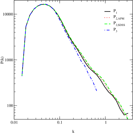
Figure 1: Present day values of three dimensional power spectra which might be inferred from angular data. The solid line ($P_{1}$) is the present value of a spectrum which (i) evolves linearly and (ii) fits the angular data. The dashed and dotted curves ($P_{2},APM$ and $P_{2},SDSS$) are the present value of a spectrum which evolves non-linearly (i.e. realistically) and fits the agnular data. The dot-dashed curve $(P_{3})$ is the linear spectrum which gives rise to the non-linear spectrum $P_{2}$. It should be used to fit cosmological parameters.

Figure 1 shows three power spectra which might conceivably be extracted from the APM survey. The three lines correspond to three different power spectra, all shown at $z=0$:

• $P_{1}$ is the power spectrum one gets from the inversion assuming linear scaling.

• $P_{2}$ has the more realistic scaling using the formalism of Peacock and Dodds, but leads to a very similar $w(\theta)$ (see figure 2). We will discuss in the next section how we arrived at this power spectrum.

• Finally $P_{3}$ is the linear spectrum associated with the non-linear spectrum $P_{2}$. That is, if the universe started with $P_{3}$ at early times (scaled back by $(1+z)^{-2}$), the non-linear power today would be $P_{2}$.

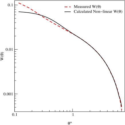
Figure 2: Measured $w$ used to fit the three-dimensional power spectrum and $w$ calculated from the fit power spectrum using the non-linear method described herein.

The first of these, $P_{1}$, is what emerges from a blind inversion assuming $P\propto(1+z)^{-2}$. This is what is usually used to compare with theories. The second, $P_{2}$, is a much more accurate extraction of the power spectrum today since we accounted for the non-linear evolution. It clearly differs from $P_{1}$ at $k\ga 0.5$, so any attempt to use $P_{1}$ to constrain cosmological parameters will necessarily be inaccurate. The only problem with $P_{2}$ is that we have not yet explained how we got it. We’ll do this in the next section. To do accurate parameter estimation, one does a best fit to the data allowing for several free parameters and evaluating the power spectrum at any point in parameter space with for example the BBKS (Bardeen et al. 1986) form or the output from CMBFAST (Seljak & Zaldarriaga 1996). To do this comparison properly, the power spectrum $P_{3}$ would need to be used, for the codes compute the linear power spectra and $P_{3}$ is the linear spectra corresponding to $P_{2}$. It has been common practice to neglect non-linear effects and simply use $P_{1}$ to fit for cosmological parameters, neglecting information on scales larger than some $k_{\rm max}$, typically chosen to be in the range $0.1-0.2h$ Mpc^-1. Since $P_{1}$ (the incorrect linear spectrum) differs from $P_{3}$ (the correct linear spectrum) at wavenumbers $k$ even smaller than $0.1h$ Mpc^-1, it would be clearly be much better to find a systematic way of obtaining $P_{3}$ or equivalently its non-linear counterpart, $P_{2}$.

4 The Weight Function

We are almost ready to divulge the secret of how we got the spectrum $P_{2}$, which we claim is a much better estimate of the power spectrum today than is $P_{1}$. First, though, let’s try to understand why the spectra $P_{1}$ and $P_{2}$ above differ. If the measurement was only of the power spectrum today, then it wouldn’t matter how the spectrum evolved with time beforehand: to fit the angular correlation function, $P_{1}$ would have to be equal to $P_{2}$ today. The difference between the two today, as reflected in figures 1 and 2, then must be due to the fact that the measurements are a weighted average of the power spectrum over time. Different surveys will carry with them different weight functions. Indeed, even different wavenumbers in the same survey will have different weight functions. It is clearly very important to understand and be able to compute the weight function.

Figure 3: The weight function $W(k,z)$ for $k=1.0,0.1,0.01h$ Mpc^-1 for both the APM survey and SDSS, which goes wider and deeper. This shows which values of $z$ contribute the most weight in the determination of the angular correlation function. The 3D power spectrum inferred therefore is $P(k,z)$ at the peak of the wave function.

The weight function can be computed by first forming a $\chi^{2}$ from the observed $\hat{w}_{i}$’s and the theoretical $w_{i}(P)$:

$$\chi^{2}\equiv\left(\hat{w}_{i}-w_{i}(P)\right)C^{-1}_{ij}\left(\hat{w}_{j}-w_{j}(P)\right)$$ (10)

where $C$ is the covariance matrix for $\hat{w}_{i}$. If we want to figure out how much weight the power spectrum at redshift $z_{\alpha}$ and wavenumber $k_{a}$ contributes to the $\chi^{2}$, we need only compute the second derivative of the $\chi^{2}$ with respect to $P_{a\alpha}$. This gives the curvature, or the weight function:

$$W(k_{a},z_{\alpha}) \equiv \frac{1}{2}{\partial^{2}\chi^{2}\over\partial P_{a\alpha}^{2}}$$ (11)

$$= \sum_{i,j}{\cal K}_{ia\alpha}C^{-1}_{ij}{\cal K}_{ja\alpha}.$$

Plugging in from eq. (2), we see that the weight function is

$$W(k,z) = \left[\frac{k(\Delta k)(\Delta z)}{2\pi}\frac{x^{4}\psi^{2}}{HF(1+z)^{6}}\right]^{2}$$

$$\times\sum_{i}C^{-1}_{ij}J_{0}(kx\sin\theta_{i})J_{0}(kx\sin\theta_{i}).$$

The weight function is plotted in figure 3 for two surveys, APM and the SDSS photometric survey. For the former, which is shallower, the weight function is peaked at $z\simeq 0.08$ and is fairly narrow. The weight function for SDSS is also shown assuming galaxies can be extracted down to $22$nd magnitude. As expected it peaks at higher redshift and is broader. For fixed $k$ we define $\bar{z}$ to be the redshift at which $W(k,z)$ peaks.

The weight functions shown in figure 3 may be somewhat suprising to those with knowledge of the surveys. The median redshifts of these surveys are larger than might be expected from consideration of figure 3. The discrepency can be attributed to the fact that, for a given $k$, quite a bit of the weight for the measurement of the power spectrum comes from large angles (and therefore reshifts much smaller than the median redshift).

The weight function gives us a very clear way to think of the power spectra extracted from the inversion. Recall that the inversion techniques assume linear scaling. Since the weight function tells us that a given $k-$ mode is mostly a measure of $P(k,\bar{z})$, we should scale back the inverted power spectrum to $\bar{z}$. Then, if we want the power spectrum today, we can scale forward with the non-linear formulae. Indeed, we can now reveal that this is how we arrived at $P_{2}$ in the previous section.

This suggests the following recipe for extracting a present day 3D power spectrum from angular data:

• Assume linear scaling so that Eq. (1) reduces to the much more managable Eq. (5).

• Invert to find $P_{1}$ today.

• Scale $P_{1}(k,z=0)$ back linearly to $P_{1}(k,\bar{z}(k))=P_{1}(k,z=0)(1+\bar{z}(k))^{-2}$. This scaled back spectrum is a good estimator for the non-linear spectrum at $\bar{z}$.

• Scale the spectrum obtained in the previous step non-linearly to its present value, $P_{2}$.

• Find the underlying linear spectrum corresponding to $P_{2}$ and $P_{3}$, call it $P_{3}$. This can then be compared to linear models to extract parameters.

5 Error on $P(k,\bar{z})$

There is one final loose end to tie up. The above prescription would be exact if the weight function was a delta-function, infinitely sharp at $\bar{z}$. Its finite width allows for the possibility that the scaling assumed around $\bar{z}$ affects the measurement of $P(k,\bar{z})$. There are several ways we can test this possibility. The first is to look at the resultant angular correlation functions from the two spectra. Figure 2 shows these and the difference between the two for APM. It is encouraging that the difference is so small. This suggests that the evolution of the power spectrum through $\bar{z}$ is not very important; the measurements are simply of $P(k,\bar{z})$.

To test this further and to assign error bars due to the assumed scaling, we can define

$$\Delta_{\rm SC}^{2}(k)\equiv\sum_{\alpha}W(k,z_{\alpha})(P_{1}(k,z_{\alpha})-P_{2}(k,z_{\alpha}))^{2}.$$ (13)

Since $\sum_{\alpha}W(k,z_{\alpha})$ is the weight of the measurement, it is the inverse of the square of the error on the measurement of $P(k)$. Therefore, $\Delta_{\rm SC}$ can be thought of as the ratio of the error due to the linear scaling assumption used in the inversion process to the overall error in the power spectrum. If $\Delta_{\rm SC}$ is much less than one, then we need not worry about the scaling assumption. Figure 4 shows that, for surveys with the depth of APM or even SDSS, $\Delta_{\rm SC}$ is indeed quite small for $k\la 1h$ Mpc^-1. The broader weight function of SDSS leads to a larger scaling error. One might argue that, even for $k$ as low as $0.3h$ Mpc^-1, the statistical error on the power spectrum is an underestimate. Taking $\Delta^{2}_{\rm SC}$ to be $0.2$ there leads suggests (assuming errors add in quadrature) that the linear evolution assumption increases the errors by a factor of $\sqrt{1+0.2}$, about ten percent. And of course, at higher wavenumbers the error bars get even larger.

Figure 4: The scaling error $\Delta^{2}_{\rm SC}$ for APM and SDSS. $\Delta_{\rm SC}$ is a measure of the error induced by assuming linear scaling to the statistical error.

6 Conclusions

The inversion of the angular correlation function gives a measure of the three-dimensional power spectrum at redshift $\bar{z}$, where $\bar{z}$ is the place where $W(k,z)$ in eq. (4) peaks. A simple way to obtain an estimate for $P(k,\bar{z})$ is to assume linear scaling of the power spectrum, invert the kernel, and scale back the power spectrum to $\bar{z}$. An estimate in the error incurred by this procedure is given by eq. (13). For current, and even future surveys, the error is small for $k<0.5h$ Mpc^-1 (but might be much more significant for deep surveys). On larger scales, the error is larger. This is not necessarily a bad thing: it is an indication that the survey is sensitive to the evolution of the power spectrum. In fact, the tools developed here could be applied to help plan surveys or devise optimal strategies for breaking a survey into subsets. One could compute the weight function for a given subset of data (e.g. a given magnitude slice) and choose a different subset whose weight function peaks far away in redshift. The width of the weight function in SDSS suggests that this may already be possible.

We have not dealt at all with the possibility of using photometric redshifts to learn more about the evolution of the power spectrum. And we have completely ignored the issue of how the galaxies are biased with respect to the matter. There has been much activity in both of these fields over the past several years, which should help extract even more useful information from angular surveys.

Acknowledgments This work is supported by NASA Grant NAG 5-7092 and the DOE.

7 References

Baugh, C.M., Efstathiou, G., 1993, MNRAS 265, 145

Baugh, C.M., Efstathiou, G., 1994, MNRAS 267, 323

Bardeen, J. M., Bond, J. R., Kaiser, N., & Szalay, A. S., 1986, ApJ , 304, 15

Dodelson, S. & Gaztañaga, E., 1999, astro-ph/9906289

Eisenstein, D. J. & Zaldarriaga, M., 1999, astro-ph/9912149

Gaztañaga, E. & Baugh, C.M., 1998, MNRAS , 294, 229

Maddox, S. J., Efstathiou, G., Sutherland, W. J., & Loveday, L. 1990, MNRAS , 242, 43P

Peacock, J. A. & Dodds, S. J., 1996, MNRAS , 280, 19

Seljak, U. & Zaldarriaga, M., 1996, ApJ 469, 437