Stellar Populations in the Large Magellanic Cloud from 2MASS

Abstract

We present a morphological analysis of the feature-rich 2MASS LMC color-magnitude diagram, identifying Galactic and LMC populations and estimating the density of LMC populations alone. We also present the projected spatial distributions of various stellar populations. The conditions that prevailed when 2MASS observed the LMC provided $10\sigma$ limiting sensitivity for $J\hbox{ \hbox to0.0pt{\raise 1.82986pt\hbox{$<$}\hss}\lower 2.79857pt\hbox{$\sim$} }16.3$, $H\hbox{ \hbox to0.0pt{\raise 1.82986pt\hbox{$<$}\hss}\lower 2.79857pt\hbox{$\sim$} }15.3$, $K_{s}\hbox{ \hbox to0.0pt{\raise 1.82986pt\hbox{$<$}\hss}\lower 2.79857pt\hbox{$\sim$} }14.7$. Major populations are identified based on matching morphological features of the color-magnitude diagram with expected positions of known populations, isochrone fits, and analysis of the projected spatial distributions.

2MASS has detected a significant population of asymptotic giant branch (AGB) stars ($\hbox{ \hbox to0.0pt{\raise 1.82986pt\hbox{$>$}\hss}\lower 2.79857pt\hbox{$\sim$} }10^{4}$ sources) and obscured AGB stars ($\hbox{ \hbox to0.0pt{\raise 1.82986pt\hbox{$>$}\hss}\lower 2.79857pt\hbox{$\sim$} }2\times 10^{3}$ sources). The LMC populations along the first-ascent red giant branch (RGB) and AGB are quantified. Comparison of the giant luminosity functions in the bar and the outer regions of the LMC shows that both luminosity functions appear consistent with each other. The luminosity function in central (bar) field has well-defined drop-off near $K_{s}=12.3^{m}$ corresponding to the location of RGB tip; the same feature is seen in the luminosity function of the entire LMC field.

Isochrone fits for the corresponding giant branches reveal no significant differences in metallicities and ages between central and outer regions of the LMC. This may be evidence for strong dynamical evolution in the last several gigayears. In particular, the observed LMC giant branch is well-fit by published tracks in the CIT/CTIO system with a distance modulus of $\mu=18.5\pm 0.1$, reddening $E_{B-V}=0.15-0.20$, metallicity $Z=0.004^{+0.002}_{-0.001}$ and age $3-13$ Gyr. Analysis of deep 2MASS engineering data with six times the standard exposure produces similar estimates.

1 Introduction

Large and homogeneous data sets of near-infrared photometry for the entire LMC, a by-product of large-scale infrared sky surveys such as 2MASS Skrutskie et al. (1997) and DENIS Epchtein et al. (1997), have become available to astronomical community only recently. Cioni et al. (2000) introduced the DENIS Point Source Catalog towards the Magellanic Clouds. Here, we present the LMC data from The Two Micron All Sky Survey (2MASS).

The 2MASS has observed the entirety of the Large Magellanic Cloud and much of these data are included in the recent second incremental data release. Empirically, the photometry has signal-to-noise (SNR) ratio 10 at J, H, K_s magnitudes of 16.3, 15.3, 14.7, respectively, slightly better than the nominal survey limit. At these limits, we can observe all of the thermally-pulsing asymptotic giant branch (AGB) populations and part way down the red giant branch (RGB). The red clump, representing helium burning giants, lies $\sim 2$ mag below the sensitivity limit of these data. The extinction in near-infrared (NIR) is small throughout the LMC and negligible on average everywhere but the inner degree of arc. Together with the high quality of 2MASS photometry ($\sigma_{m}\sim 0.03^{m}$), overall zero-point stability (better than $0.01^{m}$) and with reliable identification of LMC populations, the survey is ideal for studies of spatial structure of the LMC or its evolution (see the companion paper, Weinberg & Nikolaev 2000; hereafter WN).

We describe data selection, cross-correlation with a few well-known populations, and comparison of the 2MASS color system in §2. We present a morphological analysis the color-magnitude diagram in §3. In particular, we make identifications of the Galactic and LMC populations corresponding to all features in the color-magnitude diagram, correlate these with spatial distribution, and estimate the density of LMC populations alone. The LMC giant branch is well determined and we separately identify the AGB, first-ascent red giant branch tip (TRGB), and the carbon star sequence. The luminosity function of RGB and AGB populations is derived (§4) and compared with the galactic giant-branch luminosity function. We explore the feasibility of determining the spatial dependence of metallicity using giant-branch morphology. Finally, §5 summarizes our results and discusses the implications and opportunity for future study.

2 Data

Our LMC field is $\approx 250$ sq. degrees and covers the range from $4^{h}00^{m}$ to $6^{h}56^{m}$ in right ascension and from $-77^{\circ}$ to $-61^{\circ}$ in declination (coordinates in J2000.0). The initial sample of $7,092,894$ sources is drawn from the Working Survey Data Base and includes possible artifacts, such as filter glints and diffraction spikes from nearby bright stars, source confusion, and detection upper-limits. The known contaminants and flux statistics are well-characterized and identified during processing Cutri et al. (1999). Eliminating artifacts and requiring detections at all bands with $\sigma_{m}\leq 0.11^{m}$ (SNR $\geq 10$) leaves $1,246,304$ stars. Unlike the released catalog, these data contain multiple apparitions sources because of scan overlaps. We identify the multiple entries based on 1) spatial proximity ($|\Delta r|\leq 2^{\prime\prime}$), and 2) matching $K_{s}$-photometry ($|\Delta r|\leq 5\sigma$). Note that this procedure differs from that of the 2MASS catalog release (see Cutri et al. 1999). Our final sample contains $823,037$ sources.

The spatial distribution of these stars is shown in Figure 1. The figure shows major structural components of the LMC, the bar and disk, immersed in the field of Galactic foreground. The gradient of the foreground sources (the direction to the Galactic center is indicated by an arrow) distorts the isopleths of the outer LMC disk.

Figure 1: Distribution of 2MASS sources in the LMC field. Contour levels are labeled in units of $10^{3}$ deg^-2. Arrow points in the direction to Galactic center.

The source density near the optical center of the bar (at $\alpha=5^{h}24^{m}$, $\delta_{J2000}=-69^{\circ}44^{\prime}$) exceeds $3.6\times 10^{4}$ deg^-2. The expected mean separation among sources at this density, $\zeta=1/\sqrt{\rho}\sim 20^{\prime\prime}$, is much greater than 2MASS resolution and therefore confusion should not be significant (see also Wood 1994). As a separate check, we have examined the source counts as the function of magnitude in dense central fields and in more sparse fields in the outer LMC. The distribution of source counts as a function of magnitude have similar shapes in both dense and sparse regions, consistent with low confusion.

We have cross-correlated our sources with the database of long-period variables (LPV) from Hughes & Wood (1990). Their sample includes 376 large-amplitude Mira-like variables and 224 smaller amlitude semi-regular variables. We find 370 ($98.4\%$) and 224 2MASS counterparts, respectively. Three of the ‘missing’ large-amplitude variables are present in the raw 2MASS data, but are degraded by artifacts (two diffraction spikes and one blend). Of the remaining three, two are matched by stars of the appropriate magnitudes within $7^{\prime\prime}$ radius, and only one does not have any match to within $20^{\prime\prime}$ radius. All 134 Wolf-Rayet stars in the LMC Breysacher (1999) have been observed by 2MASS van Dyk et al. (1999).

2.1 $K_{s}$ vs. $K$ Photometry

The 2MASS photometric system is similar to CIT/CTIO system Elias et al. (1982), except that it uses $K_{s}$ band ($2.00-2.32\,\mu\rm{m}$) rather than $K$ band. The $K_{s}$ (‘K-short’) bandpass is described by Persson et al. (1998). It was designed to reduce the ground-based thermal background. The transmissivity curve for the filter is given in Persson et al., who also compared $K_{CIT}$ with $K_{s}$ photometry for a set of solar-type stars and red standards (see their Tables 2 and 3, respectively). Based on their data, the difference $K-K_{s}$ shows no significant systematic trend in the color range $0<J-K<3$. The strongest trends follow from the presence of CO-band absorption, which affects the $K$ filter more than the $K_{s}$ filter. The absolute value of the difference $|K-K_{s}|$ is less than $0.05^{m}$ and we will assume $K_{s}=K_{CIT}$ in comparing CIT/CTIO system-based stellar sequences with 2MASS data.

2.2 Interstellar Reddening

One of the advantages of 2MASS as compared to optical surveys is low interstellar reddening, since extinction at $2\mu$m is approximately 10 times smaller than in $V$. The values of interstellar reddening $E_{B-V}$ found in the literature fall in the range between $0.08$ Mateo & Hodge (1987) and $0.20$ Harris et al. (1997). The distribution of reddening from Harris et al. (1997) has non-Gaussian tail to high values. Greve et al. (1990) have reported values as high as $E_{B-V}=1.1$, found from their investigation of dust in emission nebulae in the LMC. Bessell (1991) has summarized reddening determinations from photometry, stellar polarization and HI column densities to derive foreground and intrinsic mean reddening in the Clouds. He obtained typical LMC internal reddening of $0.06$ (with substantial variations), and foreground reddening in the range $0.04-0.09$. Galactic foreground reddening can be surprisingly large in the outer regions of the LMC: Walker (1990) reported $E_{B-V}=0.18\pm 0.02$ at NGC 1841, about $15^{\circ}$ from the optical center of the LMC. On the other hand, in the cluster GLC 0435-59 (Reticulum), $11^{\circ}$ from the LMC center, the reddening is only $E_{B-V}=0.03$ Walker (1992). Zaritsky (1999) has indicated that reddening for F and G stars in the LMC is much less than that for OB stars and derived the average $<E_{B-V}>=0.03$ for late-type stars in the disk.

In the present study, the data are not dereddened. Rather, each diagram shows the direction and magnitude of the reddening vector for a specified value of $E_{B-V}$. The reddening vector is based on relations from Koornneef (1982):

$$A_{K}=0.189E_{B-V};\quad E_{J-K}=0.651E_{B-V},$$

for $R=A_{V}/E_{B-V}=3.1$. Information about the reddening may be obtained directly from 2MASS data from the analysis of the color-color diagram (see below).

3 Analysis of the Color-Magnitude Diagram

Figure 2 shows the color-color ($J-H$ vs. $H-K_{s}$) diagram of the LMC for $823,037$ 2MASS sources selected in §2. The diagram shows relatively few distinct features. The most prominent among them the extended ‘arm’ of the thermally-pulsing AGB stars (TP-AGB) in the upper right corner. Typical colors of LMC M giants are in the range $0.2\hbox{ \hbox to0.0pt{\raise 1.82986pt\hbox{$<$}\hss}\lower 2.79857pt\hbox{$\sim$} }H-K_{s}\hbox{ \hbox to0.0pt{\raise 1.82986pt\hbox{$<$}\hss}\lower 2.79857pt\hbox{$\sim$} }0.3$, $J-H\hbox{ \hbox to0.0pt{\raise 1.82986pt\hbox{$>$}\hss}\lower 2.79857pt\hbox{$\sim$} }0.8$ Frogel & Blanco (1990). Most stars on the extended arm, with colors redder than $J-K_{s}=1.6$ are carbon-rich stars Hughes & Wood (1990). Of those with the extremely red colors, $J-K_{s}>2.0$, many probably possess dusty circumstellar envelopes. The sample contains $\sim 2000$ such sources. Their locus is consistent with the track following the reddening vector for $H-K_{s}>1.0^{m}$. Figure 2 also shows fiducial color tracks for both giants and dwarfs from Wainscoat et al. (1992; hereafter W92). The two sequences overlap near $H-K_{s}=0.15$, $J-H=0.5$, since NIR colors of late G — early M type dwarfs are the same as colors of late F — early K type giants.

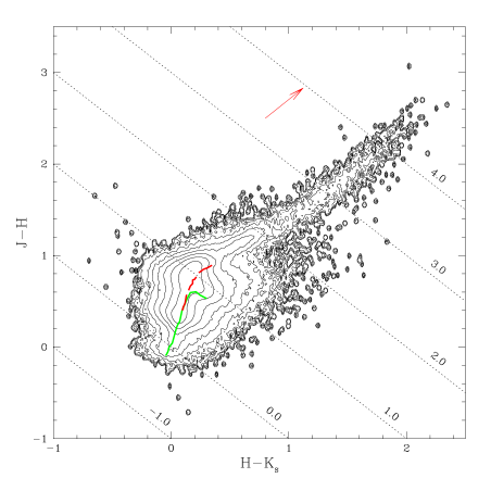
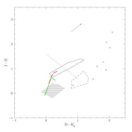
Figure 2: Left panel: Color-color diagram of the LMC field. Contour levels are logarithmic, from 2 to 6.5, spaced by 0.5. Diagonal lines are lines of constant $J-K_{s}$ values (marked). Color sequences of dwarfs (solid line) and giants (dashed line) from W92 are shown. Reddening vector for $E_{B-V}=1.0$ (indicated by arrow) is based on relations from Koornneef (1982), assuming $R=3.1$. Right panel: Color-color diagram showing approximate positions of some LMC populations. Shaded area corresponds to Wolf-Rayet stars (Breysacher 1999); region outlined by dashed lines encompasses known LMC B[e] stars (Gummersbach et al. 1995), open squares show individual observations of four LMC protostars (from Westerlund 1997). W92 fiducial colors of dwarfs (thick solid line) and giants (thick dashed line) are indicated. Region occupied by carbon stars in the sample of Costa & Frogel (1996) is shown with solid lines. Dotted line corresponds to $J-K_{s}=1.6$. Reddening vector is drawn for $E_{B-V}=1.0$.

Because of the small number of features and the general compactness of the color-color diagram, its usefulness in discriminating the major populations is limited, especially in the overlap region, $0.5<J-K_{s}<0.8$. However, some LMC populations which occupy distinct regions in the diagram can still be identified based of their location in the color-color plot (see Figure 2). In particular, the color-color diagram is quite useful in identifying candidate sources with large infrared excess, such as young protostars, cocoon stars, or obscured AGB carbon stars.

The color-color diagram may be used to determine the reddening distribution. The giant population forms a tight branch in near-infrared colors. The reddening direction nearly coincides with $J-K_{s}$ and therefore the distribution in $J-K$ of a sample from narrow color interval in $J-H$ along the giant branch provides a sensitive diagnostic for reddening by dust. We considered a sample of sources in the range $0.78<J-H<0.85$. The resulting shift of the peak is $\Delta(J-K_{s})<0.03$ ($\Delta(J-K_{s})<0.06$) outside (inside) of the central region, suggesting only minor reddening on average on scales larger than 0.1 square degrees.

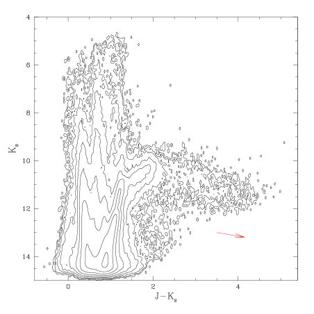
Figure 3: Left panel: Color-magnitude diagram of the LMC field. The density levels are logarithmic, from 2 to 6, spaced by 0.5. The reddening vector corresponds to $E_{B-V}=1.0$. Right panel: The same diagram with highlighted 12 regions discussed in text. The regions correspond to major features of the CMD.

The color-magnitude diagram (CMD) presented in Figure 3 reveals a wide variety of details. Our goal is reliable identification criteria for LMC stellar populations based on their positions in the diagram. The CMD is hand-shaped with vertically-stretched ‘fingers’ (e.g., at $J-K_{s}$ colors of 0.4, 0.6, 1.1) due to varying distance modulus for both Galactic and Magellanic sources. We have identified 12 regions shown in Figure 3 that highlight distinct features of the CMD. The regions are marked A through L and enclose $99.7\%$ of the $823,037$ sources in the field. To identify stellar populations in each region, we use a combination of several techniques. The Galactic foreground contribution is modeled by a synthetic CMD based on the tabulated near-infrared model of W92. The LMC populations are identified based on the infrared photometry of known populations found in the literature. In addition, we do a preliminary isochrone analysis, where we match the features of the CMD with Girardi et al. (2000) isochrones to derive the ages of populations and draw evolutionary connections among the CMD regions. The details of our population matching procedure are given in §3.1. In addition, we use the spatial density distributions of sources in each region to better discriminate local and LMC populations. The spatial distributions for each region are shown in Figure 4.

Figure 4: Spatial density distributions of sources in CMD regions. Letters correspond to the regions introduced in Figure 3. The distributions are kernel smoothed with a Gaussian kernel. The same sequence of contour levels is used in each panel (see text). Contour level of 120 deg^-2 is highlighted.

In each panel of the figure, we plot source density contour levels of 15, 30, 60, 120, 240, 350, 480, 960, 1920, 3840, 7680, and 15000 deg^-2. The contour levels are selected both to show the underlying density profiles with maximum details and facilitate the comparison among different population densities. However, due to strong variations in relative density in the CMD, not all contour levels in this sequence are displayed: in panels E and I the lowest density contour corresponds to 60 deg^-2, in panels B and C the contours start from 240 deg^-2, and in very dense Region D the lowest contour level is 960 deg^-2.

3.1 Identifying Stellar Populations

The initial analysis of the CMD regions has two parts: 1) use of the spatial density distribution to estimate the location (Galaxy or LMC); and 2) use of the theoretical colors/isochrones to derive the properties of the population, such as age, approximate spectral class and distance modulus. Here we describe the procedure of identifying the populations, before examining each region of CMD in detail.

The CMD of the LMC field (Fig. 3) contains both Galactic and LMC populations. To quantify Galactic foreground, we use near-infrared model of W92, based on 8-25 micron point source counts. Galactic model of W92 has five structural components: exponential disk, bulge, stellar halo, spiral arms and molecular ring. The main contribution to the Galactic source density toward the LMC ($l=280.5$; $b=-32.9^{\circ}$) is the exponential disk. The source density due to other Galactic structural components combined does not exceed $0.0005\%$ in any region of the CMD. The luminosity function in W92 model is represented by a sum of stellar classes, allowing independent estimate of the contribution of each class to the CMD. Each class of source is assumed to have a Gaussian distribution,

$$N(M)\propto\exp\left[-\frac{(M-M_{\lambda})^{2}}{2\sigma^{2}}\right].$$

To model the Galaxy, we use the first 33 classes from Table 2 of W92 (Galactic dwarfs, giants and supergiants). The remainder (AGBs, planetary nebulae, etc.) are expected to give only a small contribution to source density and thus do not affect the CMD. In the Galactic model, we use reddening parameters from Rieke & Lebofsky (1985). Dust is assumed to follow a double exponential distribution, with the radial scale length of the disk and the scale height of 100 pc. We reduced the magnitude dispersion $\sigma$ of each stellar class by ten to accurately represent the CMD. Reducing $\sigma$ results in a spiky differential luminosity function but this does not affect our application and the cumulative luminosity function remains well-approximated. Given the granularity of the model, the agreement between original W92 luminosity function and ours is acceptable. Our synthetic ‘foreground’ CMD is shown in Figure 5, along with the observed CMD of a Galactic field . The agreement between the model and observed CMD is good, with few easily explainable discrepancies. For example, the extension of the CMD at $J-K_{s}\hbox{ \hbox to0.0pt{\raise 1.82986pt\hbox{$>$}\hss}\lower 2.79857pt\hbox{$\sim$} }1$, $K_{s}\approx 13-14$ is due to the population of field galaxies Jarrett (1998).

Figure 5: Comparison of (a) observed CMD of a Galactic field and (b) the synthetic Galactic CMD from W92 model, as explained in text. Densities in both diagrams are normalized to unity. The contour levels are logarithmic, from $-0.5$ to $-3.5$, spaced by 0.5. Similar plots for each stellar class and for each structural component of the Milky Way allows unambiguous determination of populations responsible for observed CMD features.

Conclusions about the LMC populations in the CMD are made based on isochrone fitting or on empirical matching of populations found in the literature to features of the CMD. We use theoretical isochrones from Girardi et al. (2000). These isochrones supersede Bertelli’s set Bertelli et al. (1994), and use updated opacities and equations of state. The isochrones follow the evolution of low- and intermediate-mass stars ($0.15M_{\odot}<M<7M_{\odot}$) from the main sequence up to the tip of the RGB or the start of the thermally-pulsing AGB. Distinct LMC populations are identified by matching morphological features of the CMD with colors of known populations from the literature. In particular, we use Cepheid colors from Madore & Freedman (1991), early M supergiant color sequence from Elias et al. (1985), and data on long-period variables from Hughes & Wood (1990). This matching is purely qualitative and is only used as a supplement. The fiducial colors of Galactic giants and supergiants from W92 model are unsuitable for LMC, since LMC has a lower metallicity compared to the Milky Way. Moved to the LMC distance, $\mu=18.5$, the W92 giant branch provides a poor fit to the observed RGB (see Figure 7 below).

3.2 Region A: Blue Supergiants, O Dwarfs

These blue-colored sources are readily identified as early type Population I stars in the LMC. This group of stars is the evidence of recent ($<30$ Myr) star formation. Plotting the theoretical evolutionary tracks in the CMD (Figure 6) confirms that the region is populated by blue supergiants and brightest dwarfs (ZAMS). Only the hottest and most massive dwarfs of types O3—O6 can be seen in the LMC at $\mu=18.5$. All other main sequence (MS) populations are too faint and fall below the limit at SNR $=10$ imposed for this work. The supergiant population in the region are core helium-burning stars with masses $4\hbox{ \hbox to0.0pt{\raise 1.82986pt\hbox{$<$}\hss}\lower 2.79857pt\hbox{$\sim$} }M\hbox{ \hbox to0.0pt{\raise 1.82986pt\hbox{$<$}\hss}\lower 2.79857pt\hbox{$\sim$} }9M_{\odot}$. These stars spend most of their post-MS lifetimes as blue or red supergiants Maeder & Meynet (1989) looping between Regions A and H of the CMD (cf. Figure 6b). Region A encompasses stars which are at the blue tips of their blue loops. While crossing Regions B and C, these stars enter the instability strip and become Cepheids (see §§ 3.3, 3.4).

The spatial distribution of these objects also clearly indicates an LMC population. The distribution is rather clumpy with several richest OB associations outlining the location of spiral arms and brightest and largest HII regions (e.g., 30 Dor). The density concentrations in Fig. 4A are consistent with the well-known superassociations and Shapley’s Constellations Martin et al. (1976); van den Bergh (1981). These youngest populations do not trace the bar of the LMC, in agreement with de Vaucouleurs & Freeman (1973). Quantitative analysis of the distribution Weinberg & Nikolaev (2000) puts the centroid of the population at $\alpha=5^{h}23^{m}$, $\delta=-68^{\circ}48^{\prime}$, about $1^{\circ}$ north of the optical center of the bar.

The Galactic population of early dwarfs is readily seen in the CMD directly above Region A, blueward of Region B. The apparent magnitudes of these stars suggest a distance modulus between 5 and 10 ($r\sim 0.1-1$ kpc). In addition, this area of the CMD may also contain contribution from field blue stragglers and blue horizontal branch stars.

3.3 Region B: Galactic Disk F—K Dwarfs, LMC Supergiants

Region B is a vertically stretched band in the CMD with $J-K_{s}=0.2-0.5$. This color cut isolates the main sequence turnoff of the halo ($J-K_{s}\approx 0.3$) and the disk ($J-K_{s}\approx 0.4$). The spatial density distribution increases toward NE corner of the field (Fig. 4B), i.e. toward the Galactic center, and indicates a predominantly Galactic population. The vertical extent in the CMD indicates a wide range of distance moduli for these stars. Based on relative population abundances in our synthetic Galactic CMD, we conclude that these sources are disk dwarfs of spectral classes in the range from late F to early K. These stars account for $\sim 90\%$ of the foreground source density in the region. Their position in the CMD (see Figure 6a) suggests that the dwarfs have distance moduli $\mu=3-10$ ($r\sim 0.04-1.0$ kpc). Galactic giants in the region are of types F—G, but their contribution to foreground source density is insignificant, smaller than $5\%$.

The distorted shape of the central isopleth in Figure 4B suggests presence of the LMC population in this region. The isopleth outlines the structure similar to the one seen in the central regions in Figure 4A. Note the overdensity near $\alpha=5^{h}40^{m}$, $\delta=-69^{\circ}$ and $\alpha=5^{h}35^{m}$, $\delta=-67^{\circ}30^{\prime}$, marking positions of superassociations IV and V, respectively Martin et al. (1976). Based on the colors, the LMC component is comprised of young blue and yellow supergiants, corresponding to spectral types A—G. This population includes luminous blue variables and short period Cepheids ($P\hbox{ \hbox to0.0pt{\raise 1.82986pt\hbox{$<$}\hss}\lower 2.79857pt\hbox{$\sim$} }50^{d}$). Figure 7b shows the Cepheid sequence based on PL relations for LMC Cepheids Madore & Freedman (1991). Figure 6b also shows the colors of supergiants from W92 (Table 2). In addition, Region B contains the majority ($\hbox{ \hbox to0.0pt{\raise 1.82986pt\hbox{$>$}\hss}\lower 2.79857pt\hbox{$\sim$} }80\%$) of the known LMC Wolf-Rayet stars. Most LMC Wolf-Rayet stars have infrared colors in the range $0<J-K_{s}<0.5$. Their numbers, however, are not significant to produce an observable effect in the CMD density.

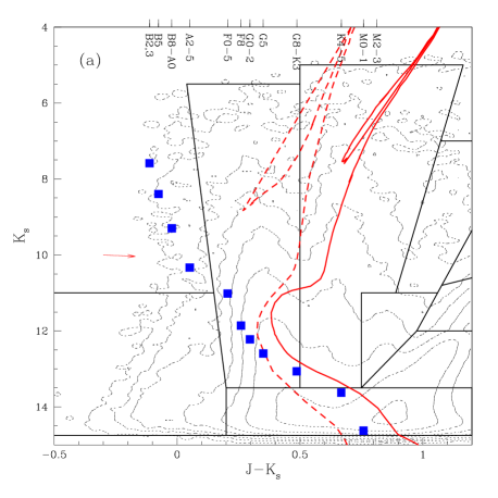
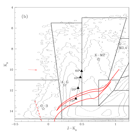
Figure 6: Part of the CMD showing Galactic and young LMC populations. (a) Galactic dwarf populations in 2MASS CMD. Solid line: theoretical isochrones for $\tau=7$ Gyr, $Z=0.019$, $\mu=9.0$, $E_{B-V}=0.1$, representing intermediate/old Galactic disk population; dashed line: isochrones for $\tau=14$ Gyr, $Z=0.0004$, $\mu=9.0$, $E_{B-v}=0.1$. Fiducial unreddened dwarf colors from W92 (for $\mu=9.0$) are indicated by filled squares, with the approximate spectral types marked in the top axis. The reddening vector corresponds to $E_{B-V}=0.2$. (b) Young LMC populations. Solid line shows the theoretical isochrone for $\tau=60$ Myr, $Z=0.008$, $\mu=18.5$, $E_{B-V}=0.2$. Empirical colors for Cepheids (Madore & Freedman 1991) are shown with triangles and mark the location of the instability strip in the diagram. Stars show fiducial color sequence of supergiants (I-II) from W92. Dashed line shows the tip of the ZAMS at $\mu=18.5$, corresponding to hottest O3-O6 dwarfs. Colors of Cepheids, supergiants and O dwarfs are unreddened. The reddening vector corresponds to $E_{B-V}=0.2$.

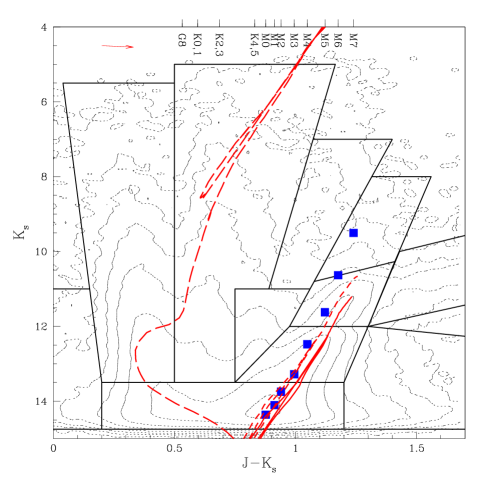
Figure 7: Part of the CMD showing intermediate and old LMC populations. Theoretical isochrones represent prototype populations — solid line: $\tau=11$ Gyr, $Z=0.004$, $\mu=18.5$, $E_{B-V}=0.2$; dashed line: $\tau=4$ Gyr, $Z=0.004$, $\mu=18.5$, $E_{B-V}=0.2$. The long-dashed line shows the isochrone for Galactic RGB stars, $\tau=9$ Gyr, $Z=0.019$, $\mu=10.0$, $E_{B-V}=0.0$. Fiducial unreddened RGB color sequence (W92) at $\mu=18.5$ is shown with squares, with approximate spectral types along the sequence marked in the top axis. The reddening vector corresponds to $E_{B-V}=0.2$.

3.4 Region C: Disk K Dwarfs and K Giants, Young Supergiants in the LMC Bar

Similar to B, Region C is stretched along the magnitude axis, indicating that the CMD feature is formed by sources at a range of distances. The colors of this population are in a tight range, $\Delta(J-K_{s})\sim 0.3$. Our synthetic Galactic CMD suggests that most ($\sim 70\%$) of the observed density in this region is produced by disk K dwarfs at $\mu<9$ ($r\hbox{ \hbox to0.0pt{\raise 1.82986pt\hbox{$<$}\hss}\lower 2.79857pt\hbox{$\sim$} }600$ pc). Disk K giants are also present in this region. Most of them have $\mu\sim 6-13$ ($r\sim 0.2-4$ kpc). They contribute $\sim 20\%$ of the foreground density. The inspection of isochrones in Figure 6a suggests that Galactic giants in this region are in the evolutionary phase of red clump/horizontal branch stars. The intrinsic brightness and color of these stars ($M_{K}=-1.4\pm 0.1$, $J-K_{s}=0.6\pm 0.1$) make them natural candidates in this region. Because of the narrow magnitude range of the clump, the source distribution in Region C along the magnitude axis could help constrain the structure of the Galactic disk.

The LMC population in Region C (seen in Figure 4C) is slightly older than youngest supergiants in Regions A, B. The central isopleths of the figure outline the bar of the LMC and show no overdensity at the positions of superassociations, seen in previous two regions. Most of the LMC sources in Region C have $K_{s}>10.5$. The similarity in the shapes of central isopleths between Fig. 4C and 4I suggests they are lower mass young supergiants with ages $300-500$ Myr, evolving into Region I (Figure 6a). These stars trace the bar of the Cloud Grebel & Brandner (1998). Some contribution from more massive supergiants, including longer-period Cepheids ($P\hbox{ \hbox to0.0pt{\raise 1.82986pt\hbox{$<$}\hss}\lower 2.79857pt\hbox{$\sim$} }100^{d}$) may also be present.

3.5 Region D: Disk G—M Dwarfs and LMC RGB and Early AGB Stars

Region D is the most heavily populated area of the CMD: it includes more than a half of all sources in the sample. Because of its position in the CMD and the large color range it spans ($0.25<J-K_{s}<1.2$), this region is also the most inhomogeneous. The spatial distribution, shown in Figure 4D shows both the foreground and LMC populations (note the distorting effect of Galactic populations on outer LMC isopleths). The observed CMD is distinctly bimodal in this region, with the red half populated by RGB and early AGB stars in the LMC, and the blue half populated mostly by G—M dwarfs in the Galaxy. The AGB stars in the red half of the region ($J-K_{s}>0.7$) are in their ‘early-AGB’ (E-AGB) phase, during which the energy is produced in the thick helium shell and outer hydrogen shell is extinguished. These stars have recently passed the base of the AGB, the so-called ‘AGB-bump’ at $K_{s}\approx 16$ that marks the transition from core to shell helium burning Castellani et al. (1991). The AGB-bump was first observed by Hardy et al. (1984) in their CMD of the LMC bar. At only $\approx 1$ mag brighter than the horizontal branch, this feature is not visible in the CMD in Figure 3 although it is present in deeper data (Figure 10). Empirically, most stars at the E-AGB are M type (oxygen-rich).

Only foreground stars are a minor contributor to the red half of Region D. (cf. Figure 5). Galactic dwarfs in this region have $\mu\sim 8-11$ ($r\sim 0.4-1.6$ kpc). Populations contributing insignificantly to the source density in this region include young supergiants, Cepheids, intermediate mass red stars in the vertically extended red clump (VRC; see §3.10).

3.6 Region E: Upper RGB and Tip of the RGB

Region E covers the upper RGB and includes the tip of the RGB (see §4). Most of these stars are on the first-ascent red giant branch; they have degenerate helium cores and hydrogen burning shells. The majority of these stars have ages anywhere between $1$ and $15$ Gyr old. The tip of the RGB is defined the helium flash, the ignition of the degenerate helium core in old (low-mass) stars (Renzini & Fusi Pecci 1989). Stars at the TRGB ignite helium in their cores and evolve rapidly to the horizontal branch. The region also contains a significant fraction of AGB stars in transition from E-AGB to TP-AGB, the stage at which the outer hydrogen shell is re-ignited Iben & Renzini (1983). During thermal pulses, the star begins alternating between hydrogen and helium shell burning. The transition from E-AGB to TP-AGB is theoretically predicted to occur near the TRGB. While on the TP-AGB, these stars may also experience the shorter-term atmospheric pulsations that lead to Mira-type variability. Analysis of MACHO data Alves et al. (1998); Wood (1999) suggests that essentially all stars brighter and redder than the TRGB are variable. Most of the E-AGB stars in this region are M stars. Extrapolated to brighter magnitudes, the sequence of oxygen-rich AGB stars extends to Regions F and G (§§3.7, 3.8).

Stars in this region of the CMD carry the most weight in our analysis of the RGB+AGB luminosity function (see §4). Their spatial distribution is relatively smooth, showing strong disk and bar components. Note the absence of significant foreground population in Figure 4E: the outer contours are elliptical in shape. A small fraction of foreground sources in this region is due to disk M dwarfs. Their density is steadily increasing toward fainter magnitudes (cf. Figure 5).

3.7 Region F: O-Rich AGBs

Region F contains primarily oxygen-rich AGB stars of intermediate age ($\hbox{ \hbox to0.0pt{\raise 1.82986pt\hbox{$>$}\hss}\lower 2.79857pt\hbox{$\sim$} }1$ Gyr) that are the descendants of stars in Region E (note the similarity between Fig. 4E and 4F). These are E-AGB and TP-AGB stars. The outer CMD isopleth in this region (Figure 3) is distorted and extends into Region J and indicates the presence of carbon stars in this region. During thermal pulses, the outer convective envelope may reach into the region where He has been transformed into C and bring carbon-enriched material to the surface. This dredge-up process leads to an increase in C/O ratio, and M stars in Regions F and G may become carbon stars. In the CMD, carbon stars form a ‘branch’ with redder colors, $J-K_{s}\hbox{ \hbox to0.0pt{\raise 1.82986pt\hbox{$>$}\hss}\lower 2.79857pt\hbox{$\sim$} }1.4$ (see §3.11). Some fraction of Region F stars are LPVs (see Figure 8) and reddened supergiants. Figures 4F and G do not show isopleths due to a Galactic population. The Galactic component in these regions are negligible because it is both too bright and too red for disk M dwarfs and too faint for Galactic AGB stars.

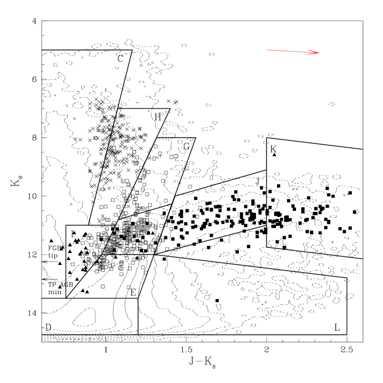
Figure 8: Portion of the CMD showing evolved stars. Crosses indicate M supergiants M1—M4 from Elias et al. (1985), solid triangles — K-type LPVs, open squares — M-type LPVs, and solid squares — C-type LPVs from Hughes & Wood (1990). Arrows at left show the theoretical tip of the RGB stars and the lower luminosity limit for thermally pulsing AGBs. The reddening vector is for $E_{B-V}=0.5$.

3.8 Region G: AGB Stars

Region G contains the most massive stars with degenerate C/O cores. This is a population of young AGB, post core-helium burning stars with initial masses between about 5-8 solar masses. These are too short-lived to become carbon stars ($0.1-1$ Gyr old), but not massive enough to become red supergiants. Similar to Region F, this region also includes LPVs (Figure 8). The period-color relation for oxygen-rich Miras derived from Feast et al. (1989) rather closely traces the young AGB branch of the CMD outlined by Regions F and G Weinberg & Nikolaev (2000). Region G lies at bright enough apparent magnitudes that the foreground density of M dwarfs is low, even in comparison to the relatively small number of O-rich luminous AGB stars in the LMC.

3.9 Region H: LMC K—M Supergiants, Galactic M Dwarfs, K—M Giants

Panel H of Figure 4 reveals an LMC population. The spatial distribution is similar to the distribution of young OB stars (Region A), suggesting that these objects are also relatively young. At $\mu=18.5$, these stars are too bright to be normal M giants. Based on their near infrared colors, we identify the Region H sources as supergiants of M type. They trace the spiral structure of the LMC and do not show significant overdensity in the bar of the Cloud, consistent with a young population. The masses of these stars are believed to be $\sim 2-9$ solar masses Bertelli et al. (1985). In the evolutionary sequence, these stars are descendants of stars in Region A (note the similarity between corresponding panels in Figure 4). These stars are also the high mass extension of the VRC.

In Figure 8, we plot the observed colors of M1—M4 supergiants from the sample of Elias et al. (1985). The colors of their sample occupy a portion of Region H, supporting our identification. The Galactic foreground consists of roughly equal contributions from disk K—M giants and M dwarfs, but their overall contribution to the source density in the region is only a few percent. This is confirmed by the absence of the Galactic isopleths in Figure 4H.

3.10 Region I: LMC Intermediate-Mass Red Supergiants, Galactic K—M Dwarfs

Region I is located at the center of the CMD, at $0.7\leq J-K_{s}\leq 1.0$. The observed overdensity in the CMD is associated with the vertically extended red clump (Zaritsky & Lin 1997). This feature consists of intermediate mass stars and is the low-mass extension of the red supergiants (Region H). The VRC extends upward from the red clump at $K_{s}\approx 17$ and becomes visible in the CMD near $K_{s}=13.5$. At the this point, the redward slope of the RGB is sufficient to distinguish the VRC.

The spatial distribution is dominated by the bar and shows traces of the spiral structure. We conclude that this LMC population is young, with the age $\hbox{ \hbox to0.0pt{\raise 1.82986pt\hbox{$<$}\hss}\lower 2.79857pt\hbox{$\sim$} }500$ Myr. The major LMC contributors to the source density in this region are K and M supergiants. This is supported by the overall similarity of LMC isopleths in Figures 4I and 4H, and also the fact that Region I is at the extension of Region H to fainter magnitudes and lower masses. Figure 8 shows K and M type Miras and SR variables in the sample of Hughes & Wood (1990). A significant fraction of their variables falls in this CMD region suggesting that some of these 2MASS stars also are variables.

The distribution in Figure 4I also reveals foreground populations. The Galactic foreground consists of M and late K dwarfs. Galactic giants contribute less than 5% of the foreground density. The dwarfs are located in the disk, with distance moduli $\mu=5-8$ ($r\sim 0.1-0.4$ kpc; Figure 6). The contribution from the Milky Way halo is smaller than 0.0005% by number for this and for all other regions of the CMD.

3.11 Region J: Carbon Stars in the LMC

At $J-K_{s}\hbox{ \hbox to0.0pt{\raise 1.82986pt\hbox{$>$}\hss}\lower 2.79857pt\hbox{$\sim$} }1.4$, Region J sources are primarily carbon-rich TP-AGB stars. These stars are descendants of oxygen-rich TP-AGBs in Regions F and G. Their outer layers are enriched in C through convection from stellar interior. As mentioned in §3.6, most of these stars are long-period variables. The variability cannot be determined based on single epoch 2MASS data, but the well-defined sequence motivates a follow-up campaign. Figure 8 shows the sample of C-rich LPVs from Hughes & Wood (1990) overplotted on the 2MASS CMD. The contamination by M-type LPVs is small. The spatial distribution of C stars in the field is similar to the distribution of their precursors (Figs. 4F). The distribution is rather smooth and shows a loop of stellar material, which has been described by Westerlund (1964). The loop is the extension of the main northern spiral arm circling the main body of the system and returning toward the bar after a nearly complete turn.

Sources in this region of the CMD offer the best opportunity to study the three-dimensional structure of the LMC for two reasons. First, the spatial coverage of the Cloud achieved by 2MASS is total and allows to probe the entire LMC. Second, as long-period variables, Region J stars are potentially good standard candles, since their intrinsic luminosity can be characterized based on their period or color. Given the selection efficiency and easily quantifiable intrinsic brightness through the period-luminosity-color relation (e.g., Feast et al. 1989), these stars are excellent probes of the LMC structure along the line of sight. Preliminary results (WN) indicate that the width of the intrinsic brightness distribution is smaller than $\sigma_{M}=0.2$ magnitudes in a narrow color range, $\Delta(J-K_{s})\sim 0.1$. At this accuracy, these standard candles can resolve features in the LMC at $\Delta r\sim 4.5$ kpc. 2MASS detected approximately $10^{4}$ potential carbon LPVs and these are sufficient to attain a reasonable confidence level in the inferred spatial structure. In Weinberg & Nikolaev (2000), we present our study of the three-dimensional structure of the LMC.

3.12 Region K: Dusty AGBs

An extension of Region J, Region K contains extremely red objects. We identify them with obscured AGB carbon-rich stars. Their large $J-K_{s}$ colors are due to dusty circumstellar envelopes ($E_{B-V}\hbox{ \hbox to0.0pt{\raise 1.82986pt\hbox{$>$}\hss}\lower 2.79857pt\hbox{$\sim$} }1$). The latter is confirmed by the appearance of their spatial and CMD distributions: (1) Figure 4K shows traces of the spiral structure outlined by these sources; and (2) the distribution in the CMD spreads from the end of Region J in the direction of reddening vector. Matching with existing near infrared photometry of obscured AGB stars in the LMC Zijlstra et al. (1996); van Loon et al. (1998) shows that most of these sources are indeed in this region of the CMD. Other extremely red populations could also be found here, e.g. ‘cocoon’ stars Reid (1991), or OH/IR stars Wood et al. (1992); van Loon et al. (1998). In addition, two of the known LMC protostars, N159-P1 and N159-P2 Jones et al. (1986) also fall in this region.

3.13 Region L: Reddened LMC M Giants, Galactic M Dwarfs and 2MASS Galaxies

Stellar sources in Region L are reddened M giants in the LMC and a small number of reddened Galactic M dwarfs. However, a significant number of sources in this region are background galaxies. The predicted CMD density in Region L due to Galactic stars is too low even after the decrease in the photometric quality near the flux limit has been taken into account; the decreasing signal-to-noise ratio causes the apparent widening of the contour levels (see Figure 5). According to Jarrett (1998), more than $90\%$ of 2MASS galaxies have colors redder than $J-K_{s}=1$.

The spatial distribution of sources (Figure 4L) shows some overdensity toward the center of the LMC. The densest part of the diagram corresponds to the position of 30 Doradus complex. Traces of spiral structure of the LMC are also visible. Based on their colors, these sources are heavily obscured RGB stars in the LMC: they lie in the direction of the reddening vector from the RGB. The inferred reddening for these sources, $E_{B-V}\sim 0.5$, is consistent with the extended tail of the LMC reddening distribution Harris et al. (1997). Region L also includes contribution from massive ($>10M_{\odot}$) protostars and ultra-compact H II regions, see Figure 8.

A population of dwarfs is implied by the outer isopleths of Figure 4L that show the increase in the direction of Galactic center. These are local M dwarfs in the disk of the Milky Way, with $\mu\sim 5-8$ ($r\sim 100-400$ pc).

4 Luminosity Function of LMC RGB and AGB Populations

We derive the LMC giant branch luminosity function (LF) from the color-magnitude diagram after subtracting Galactic foreground. Since we did not have the access to Galactic data at the time, the foreground contribution was estimated from three small fields located at the edges of our LMC field. We then scaled the resulting foreground CMD to the entire LMC field by using the estimate for the number of Galactic sources from our synthetic model. Figure 9a shows the field CMD for LMC populations only, after subtracting Galactic foreground. The expected Galactic source counts is $\sim 4\times 10^{5}$ or about $50\%$. The uncertainties in the observed CMD and in the Galactic model result in negative density regions (dotted contours) in Figure 9. The average negative density is $-10^{3.2}$ mag^-2.

The luminosity function of the LMC giants is obtained by projecting the color-magnitude diagram perpendicular to the giant branch ridge line. The function is normalized to unity. Numerical values for the RGB luminosity function are given in Table 1 and shown in the inset to Figure 9. A strong feature of the LF is a significant excess at $K_{s}\approx 12.5$, due to the TRGB. From the analysis of the derivative of the apparent luminosity function, we derive the position of the TRGB at $K_{s}=12.3\pm 0.1$. Brightward of the TRGB, the number of RGB stars drops off. The increase in the number density at the faint end, $K_{s}\hbox{ \hbox to0.0pt{\raise 1.82986pt\hbox{$>$}\hss}\lower 2.79857pt\hbox{$\sim$} }14$, is due to the increased contribution from Galactic M dwarfs (cf. Fig.5). At the bright end of the magnitude range, $11<K_{s}<12$, the luminosity function is nearly constant. It is also well above the expected number from extrapolated RGB counts. The fraction of RGB stars is small in this magnitude range and most of the stars contributing to the LF are on the AGB. As discussed above (§3.7), these stars tend to be oxygen-rich, but carbon-rich AGBs (and LPVs) are also present.

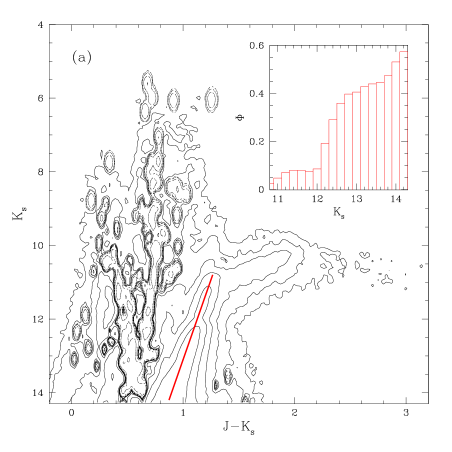
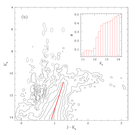
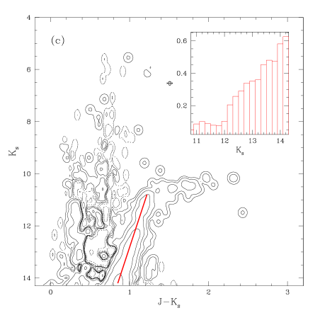
Figure 9: Color-magnitude diagrams of the LMC populations and the apparent luminosity functions of the LMC giants. Panels show CMDs of (a) entire field, (b) bar field, and (c) outer loop field (see text). The CMDs are constructed by subtracting Galactic foreground contribution from CMD in Figure 3, normalized to the same sky area. Contour levels in all panels are logarithmic, spaced by 0.5, from 2.5 to 5.5 (a), 2.0 to 4.0 (b), and from 1.0 to 3.5 (c). Dotted lines indicate negative density regions. Luminosity functions, normalized to unity, are shown in the insets of each panel.

We select two $2^{\circ}\times 1^{\circ}$ fields, one near the optical center of the bar, and the other one at $\alpha=93^{\circ}$, $\delta=-67.5^{\circ}$ (J2000.0), near the outer loop, to compare the observed M giants luminosity functions in distinct LMC environments. The outer field is probing the LMC’s outer loop delineated by the evolved stars (see §3.11). For each of the fields, we subtract the estimated Galactic foreground density scaled to the surface area of the fields. Similar to Fig. 9a, inaccuracies in both observations and models produce negative density regions. However, the average negative density in these regions is small compared to the giant branch, only $-10^{0.4}$ mag^-2 for bar region and $-10^{0.5}$ mag^-2 for loop field. Comparing the two CMDs qualitatively, we note that contribution of young OB stars and supergiants, at $J-K_{s}\hbox{ \hbox to0.0pt{\raise 1.82986pt\hbox{$<$}\hss}\lower 2.79857pt\hbox{$\sim$} }0.2$, appears stronger in the central regions of the LMC. Even though the luminosity functions in the respective fields appear different, careful analysis shows that the difference is superficial: $\chi^{2}/$d.o.f.$\approx 0.2$, which gives no motivation to entertain any difference in the parent populations. The bar LF is similar to the luminosity function of the entire field (Figure 9a), which is not surprising because the source density in the LMC field is dominated by the LMC bar. The bar luminosity function also has a pronounced TRGB at $K_{s}\approx 12.3$ and excess number density due to AGBs at $11<K_{s}<12$. The sharp increase due to Galactic M stars, seen in Figure 9a at $K_{s}\hbox{ \hbox to0.0pt{\raise 1.82986pt\hbox{$>$}\hss}\lower 2.79857pt\hbox{$\sim$} }14$, has disappeared in the bar field, because we have boosted the ratio of LMC/Galactic counts by narrowing down the field to the area of greatest LMC density. The off-bar LF shows only a mild increase in the source counts at the location of TRGB, but has the same, roughly constant profile at $K_{s}<12$, due to the AGB population, visible in the other two luminosity functions. To quantify both LFs, we present their numerical values in Table 1. The luminosity functions are given in relative units, normalized to unity. The table also gives the source counts for the LMC giant branch. For the entire LMC field we present the total counts per magnitude bin, and for the two smaller fields we give stellar density (counts mag^-1 deg^-2).

Table 1: Apparent luminosity function and source number density for the LMC giants

$K_{s}$	$\Phi$ (mag-1)a			log number density (mag-1 deg-2)
	LMC	Bar	Loop	LMCb	Bar	Loop
10.8	0.03	0.04	0.05	3.16	2.17	1.16
11.0	0.05	0.06	0.09	3.44	2.32	1.39
11.2	0.07	0.08	0.10	3.61	2.50	1.46
11.4	0.08	0.09	0.09	3.65	2.54	1.40
11.6	0.08	0.09	0.08	3.66	2.54	1.35
11.8	0.08	0.08	0.08	3.64	2.48	1.33
12.0	0.09	0.12	0.11	3.68	2.63	1.47
12.2	0.19	0.24	0.21	4.04	2.96	1.76
12.4	0.29	0.31	0.26	4.22	3.06	1.87
12.6	0.36	0.37	0.30	4.31	3.14	1.92
12.8	0.40	0.40	0.35	4.35	3.17	1.99
13.0	0.40	0.41	0.36	4.36	3.18	2.00
13.2	0.43	0.42	0.36	4.39	3.20	2.01
13.4	0.44	0.43	0.45	4.39	3.20	2.11
13.6	0.44	0.45	0.47	4.40	3.23	2.14
13.8	0.47	0.47	0.46	4.43	3.25	2.13
14.0	0.54	0.49	0.57	4.48	3.26	2.22
14.2	0.58	0.47	0.61	4.51	3.24	2.25

^aThe luminosity functions are given in relative counts per magnitude.

^bNumber density for the entire field is given as source counts per magnitude bin.

We fit theoretical isochrones Girardi et al. (2000) to each giant branch in Figure 9 to test for differences in metallicity between central and outer parts of the LMC. We chose $20$ equally-spaced grid points in $K_{s}$ magnitude between $14.3$ and $12.3$ and compute the peak in the distribution in $J-K_{s}$ at these fixed $K_{s}$ points. The difference between an isochrone (model) and the RGB (data) is characterized by the cost function (mean integrated square error):

$$f=\sum_{j}[(J-K_{s})_{j,\,RGB}-(J-K_{s})_{j,\,iso}]^{2}+w\,[K_{s}^{TRGB}-12.3]^{2},$$ (1)

where the second term is weighted measure of the match between theoretical magnitude at helium flash and observed TRGB. The weight $w$ is an adjustable parameter on the order of unity. The cost function (1) is minimized on a grid of parameter values, where the free parameters are the log-age $\tau$, metallicity $Z$, distance modulus $\mu$ and average reddening $E_{B-V}$. The best fit isochrones are as follows: $(\tau,Z,\mu,E_{B-V})=(9.8\pm 0.3,0.004^{+0.002}_{-0.001},18.45\pm 0.11,0.21\pm 0.07)$ for the central field and $(\tau,Z,\mu,E_{B-V})=(9.8\pm 0.4,0.004^{+0.002}_{-0.001},18.50\pm 0.13,0.13\pm 0.09)$ for the outer field (all errors statistical). These results imply an age range for RGB populations from $3$ to $13$ Gyr with an average of $6$ Gyr. The slope degeneracy of the isochrones in the RGB makes specific tests of star formation history difficult. In particular, our preliminary RGB isochrone analysis cannot distinguish between a continuous and single/multiple burst star formation history of the Cloud prior to approximately $4$ Gyr ago. Overall, our results do not indicate a radial metallicity gradient and provide only marginal evidence for larger reddening in central fields. The absence of strong metallicity gradients in the LMC is in agreement with results of Olszewski et al. (1991), who found no evidence for abundance gradient for cluster system. Constant C/M star ratio across the face of the LMC Westerlund (1997) and Cepheid abundances Harris et al. (1983) also support this result. Our results imply the range of abundances for field populations $-0.8<$[Fe/H]$<-0.5$, which is in good agreement with the mean abundance [Fe/H]$=-0.58\pm 0.05$ (systematic) $\pm 0.30$ (statistical) for the inner LMC disk Cole (1999). Our results agree with the disk abundance [Fe/H]$=-0.7$ Cowley & Hartwick (1982), and with results of Bica et al. (1998), who derived the range $-1.1<$[Fe/H]$<-0.4$ with the average $<[$Fe/H$]>=-0.61\pm 0.11$ from fields in the outer disk of the LMC.

The adopted detection threshold (SNR $=10$; §2) leads to the effective completeness limit of $K_{s}\approx 14.3$ in our data (cf. Figure 3). With this flux level, only the upper RGB is visible, leaving out both the AGB-bump at $K_{s}\approx 16$ and the red clump at $K_{s}\approx 17$. To resolve the giant branch down to $K_{s}\approx 16-17$, we use 2MASS engineering data, which includes six LMC scans, positioned as shown in Figure 10. Each of the ‘deep’ scans has six times the standard exposure.

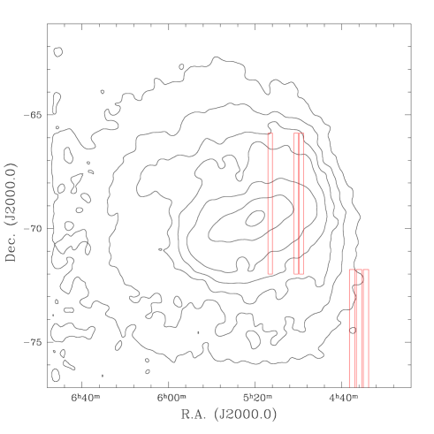
Figure 10: Positions of six ‘deep’ scans in the sky. Each scan has six times the standard integration time.

The color-magnitude diagram of the deep data is shown in Figure 11. Total number of sources in the diagram is $87,093$, of which $69,878$ ($\sim 80\%$) are in the three bar scans. Because of the bar dominance in deep data, the CMDs of the entire deep sample and the bar scans (Figs. 11a and 11b, respectively) are similar. The increased sensitivity reaches the AGB-bump at $J-K_{s}=0.7$, $K_{s}=15.8$, but still shy of the red giant clump. As with the main dataset, we quantify the deep RGB population by fitting isochrones. The resulting best fit parameters are $Z=0.004^{+0.002}_{-0.001}$, $\tau=9.7\pm 0.3$, $\mu=18.50\pm 0.12$, $E_{B-V}=0.19\pm 0.08$. The uncertainties here are statistical errors, derived from the shape of the $\chi^{2}$ surface near minimum. The range of ages for RGB populations inferred from the deep data is similar to that derived for the main data set: from $3$ to $10$ Gyr, with the average of $5$ Gyr. The other parameters are also consistent with the values derived from the regular 2MASS data. These estimates are in good agreement with recent results in the literature, e.g., the average reddening $E_{B-V}=0.20$ Harris et al. (1997); the LMC distance from Key Project, $\mu=18.5$ Mould et al. (1999); the LMC distance from TRGB, $\mu=18.59\pm 0.09$ Sakai et al. (1999).

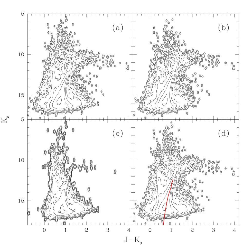
Figure 11: ‘Deep’ color-magnitude diagrams of the LMC. Panels show CMDs of (a) all six deep scans combined, (b) three bar scans, and (c) three outer field scans. Panel (d) is the same as panel (a), except also shows the best-fit isochrone for the RGB. Galactic foreground is not subtracted. The contour levels are spaced logarithmically by 0.5, from $-3.6$ to $-0.1$ (a,b,d), and from $-3.7$ to $-0.2$ (c). The lower RGB is enhanced as compared to Figure 9. Weakness of RGB in panel (c) indicates strong relative contribution from Galactic foreground. The red giant clump is just below the completeness limit in this diagram, at $K_{s}\approx 17$, $J-K_{s}\approx 0.65$.

5 Summary

In this paper, we analyzed the near-infrared CMD of the Large Magellanic Cloud and identified the major stellar populations. The populations are identified based on isochrone fitting and matching the theoretical CMD colors of known populations to the observed CMD source density. Tables 2 and 3 summarize the contents of the CMD regions.

Table 2: Regions of interest in the 2MASS CMD of the Large Magellanic Cloud.

Region	$N_{src}$	$f_{Gal}$a	Region boundaries	Dominant Spectral Typesb
A	6,659	$0.15$	$11<K_{s}<14.75$, $J-K_{s}<0.2$	B-A I-II, O3-O6 V
B	77,204	$0.80$	$5.5<K_{s}<13.5$, $0.2<J-K_{s}<0.5$	F-K V
C	62,713	$0.80$	$5<K_{s}<13.5$, $0.5<J-K_{s}\hbox{ \hbox to0.0pt{\raise 1.82986pt\hbox{$<$}\hss}\lower 2.79857pt\hbox{$\sim$} }0.8$	K V, K III
D	440,472	$0.45$	$13.5<K_{s}<14.75$, $0.2<J-K_{s}<1.2$	K-M III, F-M V
E	166,263	$0.05$	$12<K_{s}<13.5$, $0.9\hbox{ \hbox to0.0pt{\raise 1.82986pt\hbox{$<$}\hss}\lower 2.79857pt\hbox{$\sim$} }J-K_{s}\hbox{ \hbox to0.0pt{\raise 1.82986pt\hbox{$<$}\hss}\lower 2.79857pt\hbox{$\sim$} }1.2$	M III, M V
F	22,134	$0$	$10.5\hbox{ \hbox to0.0pt{\raise 1.82986pt\hbox{$<$}\hss}\lower 2.79857pt\hbox{$\sim$} }K_{s}<12$, $1\hbox{ \hbox to0.0pt{\raise 1.82986pt\hbox{$<$}\hss}\lower 2.79857pt\hbox{$\sim$} }J-K_{s}\hbox{ \hbox to0.0pt{\raise 1.82986pt\hbox{$<$}\hss}\lower 2.79857pt\hbox{$\sim$} }1.3$	M, MS
G	1,438	$0$	$8<K_{s}\hbox{ \hbox to0.0pt{\raise 1.82986pt\hbox{$<$}\hss}\lower 2.79857pt\hbox{$\sim$} }10.5$, $1.2\hbox{ \hbox to0.0pt{\raise 1.82986pt\hbox{$<$}\hss}\lower 2.79857pt\hbox{$\sim$} }J-K_{s}\hbox{ \hbox to0.0pt{\raise 1.82986pt\hbox{$<$}\hss}\lower 2.79857pt\hbox{$\sim$} }1.5$	M, MS
H	2,450	$0.05$	$7<K_{s}<11$, $1\hbox{ \hbox to0.0pt{\raise 1.82986pt\hbox{$<$}\hss}\lower 2.79857pt\hbox{$\sim$} }J-K_{s}\hbox{ \hbox to0.0pt{\raise 1.82986pt\hbox{$<$}\hss}\lower 2.79857pt\hbox{$\sim$} }1.3$	M I-II
I	21,986	$0.55$	$11<K_{s}\hbox{ \hbox to0.0pt{\raise 1.82986pt\hbox{$<$}\hss}\lower 2.79857pt\hbox{$\sim$} }13$, $0.75<J-K_{s}\hbox{ \hbox to0.0pt{\raise 1.82986pt\hbox{$<$}\hss}\lower 2.79857pt\hbox{$\sim$} }1$	K-M I-II, K-M V, M III
J	8,229	$0$	$9.5\hbox{ \hbox to0.0pt{\raise 1.82986pt\hbox{$<$}\hss}\lower 2.79857pt\hbox{$\sim$} }K_{s}\hbox{ \hbox to0.0pt{\raise 1.82986pt\hbox{$<$}\hss}\lower 2.79857pt\hbox{$\sim$} }11.5$, $1.4\hbox{ \hbox to0.0pt{\raise 1.82986pt\hbox{$<$}\hss}\lower 2.79857pt\hbox{$\sim$} }J-K_{s}<2$	C III
K	2,212	$0$	$9\hbox{ \hbox to0.0pt{\raise 1.82986pt\hbox{$<$}\hss}\lower 2.79857pt\hbox{$\sim$} }K_{s}\hbox{ \hbox to0.0pt{\raise 1.82986pt\hbox{$<$}\hss}\lower 2.79857pt\hbox{$\sim$} }13$, $2<J-K_{s}<5$	C III
L	8,940	$0.01$	$12.5\hbox{ \hbox to0.0pt{\raise 1.82986pt\hbox{$<$}\hss}\lower 2.79857pt\hbox{$\sim$} }K_{s}<14.75$, $1.2\hbox{ \hbox to0.0pt{\raise 1.82986pt\hbox{$<$}\hss}\lower 2.79857pt\hbox{$\sim$} }J-K_{s}<2.5$	M late V

^aFraction of Galactic sources estimated from synthetic W92 model

^bBased on $J-K_{s}$ color and W92; LMC populations in boldface

Table 3: LMC stellar populations in the 2MASS CMD

Stellar types	Regionsa	Typical age
Very Young
Centrally concentrated, localized to star-forming regions, trace spiral structure, weakly trace bar
O3-O6 dwarfs	A	$\hbox{ \hbox to0.0pt{\raise 1.82986pt\hbox{$<$}\hss}\lower 2.79857pt\hbox{$\sim$} }10$ Myr
Red supergiants, $5-8M_{\odot}$	H	$\hbox{ \hbox to0.0pt{\raise 1.82986pt\hbox{$<$}\hss}\lower 2.79857pt\hbox{$\sim$} }50$ Myr
Luminous AGB stars, O-rich LPVs, $M\approx 5-8M_{\odot}$	G, H, F	$\sim 40-100$ Myr
Blue and yellow supergiants, LBVs	A, B, C	$<100$ Myr
Massive protostars or cocooned OB associations	L	$\hbox{ \hbox to0.0pt{\raise 1.82986pt\hbox{$<$}\hss}\lower 2.79857pt\hbox{$\sim$} }5$ Myr
Young
Bar-dominated
Luminous E-AGB stars	G, H	$200-800$ Myr
Core He-burning giants and supergiants, $M\sim 2-5M_{\odot}$, LPVs	I, D, C, H	$100-900$ Myr
E-AGB, oxygen-rich LPVs	F, E, D	$\hbox{ \hbox to0.0pt{\raise 1.82986pt\hbox{$<$}\hss}\lower 2.79857pt\hbox{$\sim$} }1$ Gyr
Carbon stars, C-rich LPVs	J, K	$\hbox{ \hbox to0.0pt{\raise 1.82986pt\hbox{$<$}\hss}\lower 2.79857pt\hbox{$\sim$} }1$ Gyr
Intermediate and Old
Disk and bar
Low- and intermediate-mass RGB stars	D, E, L	$1-15$ Gyr
O-rich AGB stars, M-S-C stars	F	$1-4$ Gyr
C-rich TP-AGB stars	J	$1-4$ Gyr
Dust-enshrouded TP-AGB, carbon stars	K	$1-4$ Gyr
Foreground and Background
Disk populations and extragalactic component
Disk main-sequence turnoff stars	B	$\hbox{ \hbox to0.0pt{\raise 1.82986pt\hbox{$<$}\hss}\lower 2.79857pt\hbox{$\sim$} }7-9$ Gyr
Nearby K dwarfs, red clump and red HB stars	C, I	$\hbox{ \hbox to0.0pt{\raise 1.82986pt\hbox{$<$}\hss}\lower 2.79857pt\hbox{$\sim$} }9$ Gyr
Local F-M dwarfs	D, E	varies
Background galaxies	L

^aWhere a population is the dominant contributor to a region, it is labeled in bold type

The main points of this preliminary analysis of 2MASS data are the following:

• The quantity and the quality of 2MASS data allow unprecedented look at the entire LMC. 2MASS has produced a rich sample of LMC sources, a few million stars, with the photometric accuracy of 3-4%. $JHK$ 2MASS photometry is potentially useful for studying the star-formation history of the Cloud. Cross-correlating 2MASS database with existing catalogs will provide homogeneous and accurate IR photometry of supergiants (Sanduleak catalog), Wolf-Rayet stars (Breysacher catalog), Cepheids (OGLE and EROS datasets), LBVs and LPVs;

• The color-color diagram is generally ill-suited to distinguish between giant (III) and dwarf (V) populations, especially in the color range $0.5\leq J-K_{s}\leq 0.8$. Nevertheless, the diagram may be useful in identifying some candidate LMC objects with infrared excess, such as obscured AGB stars, B[e] stars, or LMC protostars. In addition, the distribution of $J-K_{s}$ colors of a population in a narrow $J-H$ color range is a sensitive reddening test;

• Major populations can be identified based on the comparison of observed CMD features with theoretical positions of known populations. Isochrone overplotting provides tentative age and metallicity estimates. We identify a substantial LMC population of AGBs ($\hbox{ \hbox to0.0pt{\raise 1.82986pt\hbox{$>$}\hss}\lower 2.79857pt\hbox{$\sim$} }10^{4}$ sources), and obscured AGBs ($\sim 2000$ sources);

• The luminosity function of the LMC giants is determined and tabulated. We find the RGB tip at $K_{s}=12.3\pm 0.1$. Our preliminary analysis of luminosity functions in two test fields suggest that luminosity function is the same in the bar and the outer regions of the Cloud;

• Fitting isochrones to the location of the giant branch (including TRGB) gives metal abundances consistent between fields. In particular, we derive average metallicity $Z=0.004^{+0.002}_{-0.001}$ for our fields. Analysis of deep data gives the same average metallicity. Our results confirm the absence of strong radial metallicity gradient in the field populations of the LMC;

• The estimates of the distance modulus obtained from our isochrone fits to the RGB, are consistent with each other and the most recent results in the literature. The average reddening is marginally different between the bar and the outer field, the $E_{B-V}$ for the bar field being greater. Distance modulus and reddening estimates from the analysis of deep data produces similar values;

• The ages of dominant RGB populations fall in the range from $3$ to $13$ Gyr, with the average age $\sim 6$ Gyr. Isochrone fits to the deep data produce similar age interval, from $3$ to $10$ Gyr, with the average age $\sim 5$ Gyr. A more detailed isochrone analysis is required to draw conclusions about the history of star formation in the LMC prior to $3-4$ Gyr ago;

• Carbon-rich long-period variables are noted as potential standard candles. Due to their significant numbers and narrow luminosity range (which may be parametrized through a period-luminosity or luminosity-color relations), these stars are ideally suited for studying the structure of the LMC along the line of sight.

References

- Alves et al. (1998) Alves, D., Alcock, C., Cook, K., Marshall, S., Minniti, D., Allsman, R., Axelrod, T., Freeman, K., Peterson, B., Rodgers, A., Griest, K., Vandehei, T., Becker, A., Stubbs, C., Tomaney, A., Bennett, D., Lehner, M., Quinn, P., Pratt, M., Sutherland, W., Welch, D. 1998, in Pulsating Stars: Recent Developments in Theory and Observation, Proceedings of IAU Joint Discussion 24, eds. M. Takeuti & D. Sasselov (Tokyo:Universal Academy Press)
- Bertelli et al. (1985) Bertelli, G, Bressan, A. G., Chiosi, C. 1985, A&A, 150, 33
- Bertelli et al. (1994) Bertelli, G., Bressan, A., Chiosi, C., Fagotto, F., Nasi, E. 1994, AAS, 106, 275
- Bessell (1991) Bessell, M. S. 1991, A&A, 242, L17
- Bica et al. (1998) Bica, E., Geisler, D., Dottori, H., Clariá, J. J., Piatti, A. E., Santos, J. F. C., Jr., 1998, AJ, 116, 723
- Breysacher (1999) Breysacher, J., Azzopardi, M., Testor, G. 1999, AAS, 137, 117
- Castellani et al. (1991) Castellani, V., Chieffi, A., Pulone, L. 1991, ApJS, 76, 911
- Cioni et al. (2000) Cioni, M.-R., Loup, C., Habing, H. J., Fouqué, P., Bertin, E., Deul, E., Egret, D., Alard, C., de Batz, B., Borsenberger, J., Dennefeld, M., Epchtein, N., Forveille, T.,Garzón, F., Hron, J., Kimeswenger, S., Lacombe, F., Le Bertre, T., Mamon, G. A., Omont, A., Paturel, G., Persi, P., Robin, A., Rouan, D., Simon, G., Tiphène, D., Vauglin, I., Wagner, S. 2000, accepted to A&A
- Cole (1999) Cole, A. A. 1999, Ph.D. thesis, University of Wisconsin-Madison
- Costa & Frogel (1996) Costa, E. & Frogel, J. A. 1996, AJ, 112, 2607
- Cowley & Hartwick (1982) Cowley, A. P. & Hartwick, F. D. A. 1982, ApJ, 259, 89
- Cutri et al. (1999) Cutri, R. M, Skrutskie, M. F., Van Dyk, S., Chester, T., Evans, T., Fowler, J., Gizis, J., Howard, E., Huchra, J., Jarrett, T., Kopan, E. L., Kirkpatrick, J. D., Light, R. M, Marsh, K. A., McCallon, H., Schneider, S., Stiening, R., Sykes, M., Weinberg, M., Wheaton, W. A., Wheelock, S. 1999, [http://www.ipac.caltech.edu/2mass/releases/first/doc/explsup.html]
- Elias et al. (1982) Elias, J. H., Frogel, J. A., Matthews, K, Neugebauer, G. 1982, AJ, 87, 1029
- Elias et al. (1985) Elias, J. H., Frogel, J. A., Humphreys, R. M. 1985, ApJS, 57, 91
- Epchtein et al. (1997) Epchtein, N., de Batz, B., Capoani, L., Chevallier, L., Copet, E., Fouqué, P., Lacombe, F., Le Bertre, T., Pau, S., Rouan, D., Ruphy, S., Simon, G., Tiphène, D., Burton, W. B., Bertin, E., Deul, E., Habing, H., Borsenberger, J., Dennefeld, M., Guglielmo, F., Loup, C., Mamon, G., Ng, Y., Omont, A., Provost, L., Renault, J.-C., Tanguy, F., Kimeswenger, S., Kienel, C., Garzón, F., Persi, P., Ferrari-Toniolo, M., Robin, A., Paturel, G., Vauglin, I., Forveille, T., Delfosse, X., Hron, J., Schultheis, M., Appenzeller, I., Wagner, S., Balazs, L., Holl, A., Lepine, J., Boscolo, P., Picazzio, E., Duc, P.-A., Mennessier, M.-O. 1997, The Messenger, 87, 27
- Feast et al. (1989) Feast, M. W., Glass, I. S., Whitelock, P. A., Catchpole, R. M. 1989, MNRAS, 241, 375
- Frogel & Blanco (1990) Frogel, J. A. & Blanco, V. M. 1990, ApJ, 365, 168
- Girardi et al. (2000) Girardi, L., Bressan, A., Bertelli, G., Chiosi, C. 2000, AAS, 141, 371
- Grebel & Brandner (1998) Grebel, E. K. & Brandner, W. 1998, in The Magellanic Clouds and Other Dwarf Galaxies, Proceedings of the Bonn/Bochum-Graduiertenkolleg Workshop, Germany, January 19-22, eds. T. Richtler and J. M. Braun, p.151
- Greve et al. (1990) Greve, A., van Genderen, A. M., Laval, A. 1990, AAS, 85, 895
- Gummersbach et al. (1995) Gummersbach, C. A., Zickgraf, F.-J., Wolf, B. 1995, A&A, 302, 409
- Hardy et al. (1984) Hardy, E., Buonanno, R., Corsi, C. E., Janes, K. A., Schommer, R. A. 1984, ApJ, 278, 592
- Harris et al. (1983) Harris, H. C. 1983, AJ, 88, 507
- Harris et al. (1997) Harris, J., Zaritsky, D., Thompson, I. 1997, AJ, 114, 1933
- Hughes & Wood (1990) Hughes, S. M. G. & Wood, P. R. 1990, AJ, 99, 784
- Iben & Renzini (1983) Iben, I., Jr. & Renzini, A. 1983, ARA&A, 21, 271
- Jarrett (1998) Jarrett, T. 1998, [http://spider.ipac.caltech.edu/staff/jarrett/2mass/3chan/colors/color_ crit.html]
- Jones et al. (1986) Jones, T. J., Hyland, A. R., Straw, S., Harvey, P. M., Wilking, B. A., Joy, M., Gatley, I., Thomas, J. A. 1986, MNRAS, 219, 603
- Koornneef (1982) Koornneef, J. 1982, A&A, 107, 247
- Madore & Freedman (1991) Madore, B. F & Freedman, W. L. 1991, PASP, 103, 933
- Maeder & Meynet (1989) Maeder, A. & Meynet, G. 1989, A&A, 210, 155
- Martin et al. (1976) Martin, N., Prévot, L., Rebeirot, E., Rousseau, J. 1976, A&A, 51, 31
- Mateo & Hodge (1987) Mateo, M. & Hodge, P. 1987, ApJ, 320, 626
- Mould et al. (1999) Mould, J. R., Huchra, J. P., Freedman, W. L., Kennicutt, R. C., Jr, Ferrarese, L., Ford, H. C., Gibson, B. K., Graham, J. A., Hughes, S., Illingworth, G. D., Kelson, D. D., Macri, L. M, Madore, B. F., Sakai, S., Sebo, K., Silbermann, N. A., Stetson, P. B. 1999, astro-ph/9909260
- Olszewski et al. (1991) Olszewski, E. W., Schommer, R. A., Suntzeff, N. B., Harris, H. C. 1991, AJ, 101, 515
- Persson et al. (1998) Persson, S. E., Murphy, D. C., Krzeminski, W., Roth, M., Rieke, M. J. 1998, AJ, 116, 2475
- Reid (1991) Reid, N. 1991, ApJ, 382, 143
- Renzini & Fusi Pecci (1989) Renzini, A. & Fusi-Pecci, F. 1988, ARA&A, 26, 199
- Rieke & Lebofsky (1985) Rieke, G. H. & Lebofsky, M. J. 1985, ApJ, 288, 618
- Sakai et al. (1999) Sakai, S., Zaritski, D., Kennicutt, R., 1999, astro-ph/9911528
- Skrutskie et al. (1997) Skrutskie, M. F., Schneider, S. E., Stiening, R., Strom, S. E., Weinberg, M. D., Beichman, C., Chester, T., Cutri, R., Lonsdale, C., Elias, J., Elston, R., Capps, R., Carpenter, J., Huchra, J., Liebert, J., Monet, D., Price, S., Seitzer, P., in The Impact of Large Scale Near-IR Sky Surveys, p.187, F. Garzon et al. (eds.), Kluwer (Netherlands).
- de Vaucouleurs & Freeman (1973) de Vaucouleurs, G. & Freeman, K. C. 1973, Vis. Astron., 14, 163
- van den Bergh (1981) van den Bergh, S. 1981, AAS, 46, 79
- van Dyk et al. (1999) van Dyk, S. D., Cutri, R., Skrutskie, M. F. 1999, BAAS, 195.0403
- van Loon et al. (1998) van Loon,J. Th., Zijlstra, A. A., Whitelock, P. A., Te Lintel Hekkert, P., Chapman, J. M., Loup, C., Groenewegen, M. A. T., Waters, L. B. F. M., Trams, N. R. 1998, A&A, 329, 169.
- Wainscoat et al. (1992) Wainscoat, R. J., Cohen, M., Volk, K., Walker, H. J., Schwartz, D. E. 1992, ApJS, 83, 111 (W92)
- Walker (1990) Walker, A. R. 1990, AJ, 100, 1532
- Walker (1992) Walker, A. R. 1992, AJ, 103, 1166
- Weinberg & Nikolaev (2000) Weinberg, M. D. & Nikolaev, S. 2000, in preparation
- Westerlund (1964) Westerlund, B. E. 1964, in The Galaxy and the Magellanic Clouds, Proceedings of the IAU Symp. 20, edited by F. J. Kerr, p. 239
- Westerlund (1997) Westerlund, B. E. 1997, The Magellanic Clouds, Cambridge University Press
- Wood et al. (1992) Wood, P. R., Whiteoak, J. B., Hughes, S. M. G., Bessell, M. S., Gardner, F. F., Hyland, A. R. 1992, ApJ, 397, 552
- Wood (1994) Wood, P. R. 1994, Ap&SS, 217, 121
- Wood (1999) Wood, P. R. 1999, private communication
- Zaritsky & Lin (1997) Zaritsky, D., Lin, D. N. C. 1997, AJ, 114, 2545
- Zaritsky (1999) Zaritsky, D. 1999, AJ, 118, 2824
- Zijlstra et al. (1996) Zijlstra, A. A., Loup, C., Waters, L. B. F. M., Whitelock, P. A., van Loon, J. Th., Guglielmo, F. 1996, MNRAS, 279, 32