Post-glitch RXTE-PCA observations of the Vela pulsar

Abstract

We report the results of analysis of observations of the Vela Pulsar by PCA on RXTE. Our data consists of two parts. The first part contains observations at 1, 4, and 9 days after the glitch in 1996 and has 27000 sec. total exposure time. The second part of observations were performed three months after this glitch and have a total exposure time of 93000 sec. We found pulsations in both sets. The observed spectrum is a power-law with no apparent change in flux or count rate. The theoretical expectations of increase in flux due to internal heating after a glitch are smaller than the uncertainty of the observations.

1 Introduction

We present observations of the Vela pulsar with the Proportional Counter Array (PCA), on the Rossi X-Ray Timing Explorer (RXTE). Our observations cover two distinct time-spans. The first part is very close to the glitch on 1996 October 13.394 UT (Flanagan glidate (1996)). It consists of three observations at one, four and nine days after the glitch. We analyzed these sets of data separately. The second series of observations were obtained in January 1997. All data sets of January 1997 were analyzed together. The exact dates of observations are given in Table 1.

We first performed spectral analysis of our data, calculated time averaged flux for different observations and put upper limits for the flux change. Then, by using radio ephemerides, we detected the pulsations in the data, and investigated the changes in pulse shape and pulse fraction. Finally, we compared our results with the theoretical expectations of change in flux which might arise because of glitch induced energy dissipation in the neutron star.

Time averaged spectrum analysis is explained in section 2. The detected pulse shapes are presented in section 3. In section 4 we discuss the implications of our results.

2 Time Averaged Spectrum Analysis

The observation time-spans, and total integration times are given in Table 1 together with calculated model parameters, and flux values. The analysis is carried out using FTOOLS 4.1.1 and XSPEC v10. Only the data coming from the first xenon layer was chosen to increase the signal-to-noise ratio. The time intervals in which one or more of the five Proportional Counting Units (PCUs) are off, the elevation angle is less than 10 degrees, or pointing offset is greater than 0.02 degrees were not included in the analysis, as recommended in the “Screening” section of “ABC of XTE” (RXTE GOF abcxte (1998)). The background used is synthetic and is generated by the background estimator pcabackest. The background models are based on rate of very large events, spacecraft activation, and cosmic X-ray emission. More information on background models can be found in (Jahoda jaho (1996)). We have used the 2.2.1_v80 version of response matrices. Although the matrices are not equally good for each PCU, to have good statistics, we combined data coming from every PCU, contrary to the recommendation by Remillard (remi_resp (1997)).

A comparison of background with the data led us to ignore the channels above 68, which approximately corresponds to the energy 25.7 keV (see Fig. 1.). The systematic errors were chosen to make the reduced $\chi^{2}$ equal to unity in XSPEC. To have reasonable systematic errors we also had to ignore channels 0-7. The maximum energy for the seventh channel is 2.90 keV.

Figure 1: Number of counts versus channel for the data and the background. After around channel 68 the data and the background coincide.

The hydrogen column density model used by XSPEC is valid for the energies 0.03-10 keV. Although this covers the ROSAT energy band (0.5-2.4 keV), major portion of our spectrum (2.90-25.7 keV) falls outside this range. Therefore, we adopted the hydrogen column density $4\times 10^{20}\hbox{atoms}/\hbox{cm}^{2}$ obtained in a ROSAT observation of the Vela pulsar (Ögelman et al. vel_og (1993)), since at lower energies the spectral resolution of ROSAT is much better than RXTE/PCA detectors’ resolution.

Figures 2 and 3 are plots of the energy spectrum along with fitted models and residuals. The model parameters are given in Table 1. The quoted errors are for three sigma confidence levels. The calculated flux for each observation along with an upper and a lower limit are given in Table 1. The upper (lower) limits for the flux are calculated by setting the index of the power-law to the lower (upper) limits given by XSPEC, leaving the normalization of the power-law spectrum as the only free parameter, and refitting the spectrum.

Figure 2: Spectra of observations 10276-01-01-00, 10276-01-02-00, and 10276-01-03-00. The horizontal axis is energy in keV, the vertical axis shows counts/sec/keV (upper panel) and calculated residuals (lower panel). The solid line denotes the fitted model (photon absorbed power-law).

Figure 3: Spectra of observations 10275-01-01-00, 10275-01-01-03, and 10275-01-01-06. The horizontal axis is energy in keV, the vertical axis shows counts/sec/keV (upper panel) and calculated residuals (lower panel). The solid line denotes the fitted model (photon absorbed power-law). The results obtained from other observations in January 1997 are very similar to these presented results.

Table 1: Parameters for the observations. The third column is the total time devoted to the observation in seconds. The power-law index values have three $\sigma$ confidence levels. The unit for flux is $10^{-10}\hbox{ergs}\,\hbox{cm}^{-2}\hbox{sec}^{-1}$. The last column is the percent systematic error.

Observation ID	Date	time	power-law	Flux for 2-20 keV			sys.
		(secs)	index	Low Lim.	Value	Up Lim.	err.
10276-01-01-00	14/10/96	8434	$2.073^{2.101}_{2.045}$	2.735	2.741	2.747	1.8
10276-01-02-00	17/10/96	8762	$2.024^{2.038}_{2.008}$	2.801	2.805	2.804	0.7
10276-01-03-00	22/10/96	9601	$2.067^{2.092}_{2.044}$	2.758	2.763	2.768	1.6
10275-01-01-00	17/01/97	17707	$2.077^{2.107}_{2.046}$	2.697	2.707	2.716	2.1
10275-01-01-01	22/01/97	14808	$2.066^{2.091}_{2.039}$	2.712	2.719	2.725	1.7
10275-01-01-02	17/01/97	5363	$2.071^{2.100}_{2.041}$	2.713	2.718	2.722	1.8
10275-01-01-03	18/01/97	6601	$2.060^{2.086}_{2.033}$	2.722	2.724	2.727	1.5
10275-01-01-04	23/01/97	8411	$2.059^{2.083}_{2.034}$	2.715	2.719	2.722	1.5
10275-01-01-05	13/01/97	7228	$2.045^{2.064}_{2.025}$	2.739	2.739	2.740	1.0
10275-01-01-06	12/01/97	4379	$2.044^{2.065}_{2.022}$	2.708	2.711	2.713	1.0
10275-01-01-07	20/01/97	11695	$2.062^{2.085}_{2.037}$	2.710	2.714	2.719	1.5
10275-01-01-08 & 080	21/01/97	16765	$2.070^{2.095}_{2.044}$	2.716	2.723	2.730	1.7

We have also searched for a blackbody component to the spectrum in addition to power-law, but this resulted in temperatures $\sim\!\!10$ times larger than what has been found by Ögelman et al. (vel_og (1993)), for all observations. Although the addition of a blackbody component improves the fit, the resulting temperature suggests that this is not physical but merely a result of an increase in the number of variables. This idea is supported by the fact that adding a bremsstrahlung component to power-law or changing the power-law to a broken power-law gives a fit as good as a power-law blackbody combination.

3 Timing Analysis

The data analyzed consists of two parts. The earlier data sets extend between one and ten days after the glitch, where the post-glitch exponential relaxation of the pulse period prevails. The second data set, about three months after the glitch, does not display this rapid variation of the pulse frequency.

Figure 4: Pulse shapes obtained for the observations. $y$-axis is number of photon counts, $x$-axis is twice the phase. The photon counts include all photons detected in the first layer, channels 8-68 inclusive (2.90-25.7 keV). No background subtraction was done. A single, typical error bar is displayed for each set. (a) and (b) are the first two observations just after the glitch, these curves are obtained by interpolating values of frequency and frequency derivative given by the ephemerides. (c) and (d) are the second and third observations, these curves are obtained by polynomial fit to values given in the Princeton ephemerides. (e) represents all the observations three months after the glitch, this curve is obtained by using the values given in the Princeton ephemerides.

Finding a pulsation in the latter was straightforward. By using the Princeton ephemerides distributed with FTOOLS the pulse shape shown in Fig. 4(e) is obtained. This is a histogram of counts versus twice the phase, which is divided into 22 intervals. The histogram includes all photons detected in the first layer and in channels 8-68 inclusive. No filtering was done for elevation, offset or number of PCUs. Since background is synthetic it is not subtracted either.

Finding a pulse for earlier observations, which are very close to the glitch, proved to be difficult. There are two sets of ephemerides in the Princeton database that are relevant to these observations, and an additional one was provided by Claire Flanagan (private communication). The first two give the frequency, frequency derivative, and frequency second derivative, while the third one gives only frequency and frequency derivative. The time-spans covered by these ephemerides and the three observations in the earlier set are shown in Fig. 5. The reference epoch of the ephemerides are roughly 50370.7, 50372.0, and 50379.0 for Flanagan and Princeton ephemerides one and two, respectively. None of the ephemerides by itself gives a pulse for any of the three observations. Furthermore the ephemerides give different results for overlapping portions.

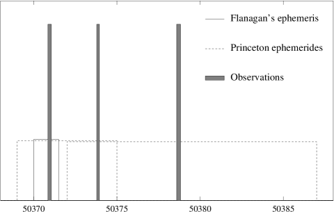
Figure 5: Observation and ephemerides time-spans. The rectangular spikes match the duration of the observations. Solid line is ephemeris provided by Flanagan. Dashed lines denote Princeton ephemerides. The horizontal axis is marked in Modified Julian Day.

We therefore tried to combine the ephemerides. We interpolated the values of frequency and frequency derivative by making a second order polynomial fit to the values given in the ephemerides. This yielded to the expressions:

$$f = .2975280743\times 10^{-18}t^{2}$$ (1)

$$-.16020626525\times 10^{-10}t+11.1962177095,$$

$$\dot{f} = -.242915\times 10^{-23}t^{2}$$ (2)

$$+.242121\times 10^{-17}t-.1622\times 10^{-10}\!\!.$$

The epoch for these expressions is the same Flanagan’s ephemeris. By using these values and not taking the higher derivatives into account, we calculated the phase for the arrival time of each photon. This method yielded reasonable pulse shapes for the first and second observation (see Fig. 4 (a) and (b) ), but failed for the third one. The reference epoch of the second Princeton ephemeris is very near to the third observation, nevertheless the use of the ephemeris which represents an extended time-span of rapidly varying periods, fails to give a pulse shape by itself. We therefore tried another approach. We combined the frequencies, frequency derivatives, and frequency second derivatives given in the two Princeton ephemerides, made a fifth order polynomial fit, and threw away the fourth and fifth order terms. In this way we reduced the contribution of the second ephemeris. The final expression for frequency is:

$$f = -9.68274932\times 10^{-25}t^{3}+0.8\times 10^{-18}t^{2}$$ (3)

$$-1.59821\times 10^{-11}t+11.1962159427143.$$

The epoch for this expression is the same as first Princeton ephemeris. The pulse shapes obtained for the second and third observations by this method are given in Fig. 4 (c) and (d).

4 Conclusions and Discussion

4.1 Time Averaged Spectrum

The power-law spectrum observed is in agreement with expectations deduced from previous observations of Vela at higher and lower energies(Ögelman et al. vel_og (1993), Kanbach et al. kanbach (1994), Strickman et al. strick96 (1996), Kuiper et al. kuiper (1998) ). At this part of spectrum (2-20 keV), the contribution of the pulsar is very small compared to the contribution of the compact nebula surrounding it. As a result the pulse shapes have a very high DC level, as can be seen in Fig. 4.

The slightly higher residuals near 6 keV and lower residuals near 4 keV are not characteristics of observed sources, but are artifacts of PCA. This effect, which is a result of the L edge of Xenon, is reduced by the version of response matrices in use, but not completely removed.

Our main conclusion from the analysis is that the spectrum does not change from early post-glitch to late observations. It is a power-law with an index around 2 for all of the observations. The power-law index does not change significantly among the observations. The highest value calculated for the index is 2.107 and the lowest value is 2.009. This corresponds to a change of 5%, which is a fractional upper limit for the change of power-index during the observations.

The upper and lower limits of the flux calculated by the comparison explained in section 2 and presented in Table 1 are well within the range of systematic errors. We therefore adopt the systematic errors as the upper limits to any variation in flux.

There is seemingly a jump in the flux between 2-20 keV, from the first to the second observation. This observation is only four days away from the glitch. The pre-glitch temperature of the surface of the Vela pulsar is thought to be around 0.15 keV(Ögelman et al. vel_og (1993)). Theoretical models (Van Riper et al.nsth1 (1991); Umeda et al.nsth2 (1993); Hirano et al. nsth3 (1997)) predict an increase at most by a factor of 8, which brings the temperature to 1.2 keV. Attempts to find a blackbody component in this observation did not give significantly different results from other observations. This suggests that the observed flux changes may have little or nothing to do with changes in surface temperature.

Another possible interpretation is that there is an error in the analysis of this particular observation, possibly arising from the calculation of synthetic background. Vela is a faint source for PCA. An improved model in the estimation of background for faint sources has been released by the PCA Team in 1998. This model has been used throughout the calculations. There may be further improvements on the background models that could change the calculated flux. The presented flux is calculated by using the spectrum model, rather than by direct observation. Apart from this observation there is no apparent change in flux or count rate.

Treating the calculated fluxes as very high upper bounds to the Wien tail of possible blackbody radiation from the neutron star surface could in principle be used to rule out some of the models for the post-glitch thermal emission from the neutron stars. In practice this does not work since the surface temperature range of the Vela pulsar is far below the RXTE-PCA energies.

4.2 Timing Analysis and Pulse Shapes

The epoch of the second ephemeris taken from the Princeton database, 50379.0 MJD, is pretty close to the third observation (see Fig. 5), but using the ephemeris alone for the observation does not give a pulse shape. This may be due to the existence of two distinct decay time scales of Vela, 3 days and 30 days, which were observed in all previous glitches and fall within the ranges of ephemeris (Alpar et al. Alpar93 (1993)). Our data is not good enough to determine any exponential decay time scales.

In view of the rapidly varying period at those epochs, the pulse shapes of the first part of the observations were obtained by a careful interpolation amounting to the construction of an ephemeris that can represent the rapid changes in the pulsar’s timing parameters in this postglitch epoch. The phase difference of the two observed peaks in these shapes is the same as the phase difference in the second set of observations (in January 1997). This gives us some confidence in the resultant pulse shapes.

The pulse shapes obtained are not reliable for drawing conclusions on the changes of pulse shape or pulsed fraction, since both of these factors are sensitively dependent on ephemeris. This is best seen by comparing Fig. 4 (b) and (c). They belong to the same set of data but have obvious differences both in the pulse shape and pulsed fraction.

4.3 Possible Future Work

Extracting the contribution of the compact nebula from the spectrum may help to delineate effects of temperature changes on the neutron star surface. Although the pulsations are detected, they are not reliable enough to justify taking the off-peak photon counts as background to the peak photon counts to remove the effects coming from the DC signal. The field of view of the PCA detector is one degree (RXTE GOF PCA (1996)), consequently the compact nebula surrounding the Vela pulsar has a significant contribution to the observed spectrum. The images showing the emission from the pulsar and the sources around it, in particular the compact nebula, can be found in Markwardt (craig_neb (1998)), Frail et al. (ogel2 (1997)), Harnden et al. (1985 (1985)), and Willmore et al. (willmore (1992)).

When we divided the data from the second part of observations into smaller time intervals we have observed that the pulse shape begins to disappear for data strings covering less than 30000 seconds. The exposure time of the data sets we used in this work are below 10000 seconds. This explains the uncertainty in pulse shapes and fractions. Future target of opportunity observation of the Vela pulsar by RXTE need to be allocated more observation time, and should contain observations made approximately 20 days after the glitch, since this is about the time that the surface temperature will reach its maximum according to theoretical models. Also, more detailed ephemerides fitting the post-glitch behavior of the pulsar is necessary to make deductions on changes in pulse shape.

Finally we note that the question of glitch associated energy dissipation in the Vela pulsar has been addressed also with ROSAT observations. Comparison of observations at epochs before and after the glitch has not yielded stringent constraints on the glitch related energy dissipation (Seward et al. ROSAT (1999)).

While this work was in preparation another analysis of RXTE/PCA observations of the Vela pulsar was published by Strickman et al. (strick2 (1999)). They have also detected a pulsed emission and a power-law spectrum. Our analysis differs from theirs in two ways. Their phase-resolved spectra are obtained by taking “off-pulse” photons as background to “on-pulse” photons, whereas we calculated only time averaged spectra. Another difference is that these authors used data coming from only the first xenon layer for energies below 8 keV, but included data coming from the other two layers for higher energies. In our analysis we used photons detected only in the first xenon layer. As a result of these differences, their power-law index is smaller than the value that we found.