Non-Uniform Reionization by Galaxies and its Effect on the Cosmic Microwave Background

Abstract

We present predictions for the reionization of the intergalactic medium (IGM) by stars in high-redshift galaxies, based on a semi-analytic model of galaxy formation. We calculate ionizing luminosities of galaxies, including the effects of absorption by interstellar gas and dust on the escape fraction $f_{\rm esc}$, and follow the propagation of the ionization fronts around each galaxy in order to calculate the filling factor of ionized hydrogen in the IGM. For a $\Lambda{\rm CDM}$ cosmology, with parameters of the galaxy formation model chosen to match observations of present-day galaxies, and a physical calculation of the escape fraction, we find that the hydrogen in the IGM will be reionized at redshift $z=6.1$ if the IGM has uniform density, but only by $z=4.5$ if the IGM is clumped. If instead we assume a constant escape fraction of 20% for all galaxies, then we find reionization at $z=9.0$ and $z=7.8$ for the same two assumptions about IGM clumping. We combine our semi-analytic model with an N-body simulation of the distribution of dark matter in the universe in order to calculate the evolution of the spatial and velocity distribution of the ionized gas in the IGM, and use this to calculate the secondary temperature anisotropies induced in the cosmic microwave background (CMB) by scattering off free electrons. The models predict a spectrum of secondary anisotropies covering a broad range of angular scales, with fractional temperature fluctuations $\sim 10^{-7}-10^{-6}$ on arcminute scales. The amplitude depends strongly on the total baryon density, and less sensitively on the escape fraction $f_{\rm esc}$. The amplitude also depends somewhat on the geometry of reionization, with models in which the regions of highest gas density are reionized first giving larger CMB fluctuations than the case where galaxies ionize surrounding spherical regions, and models where low density regions reionize first giving the smallest fluctuations. Measurement of these anisotropies can therefore put important constraints on the reionization process, in particular, the redshift evolution of the filling factor, and should be a primary objective of a next generation submillimeter telescope such as the Atacama Large Millimeter Array.

1 Introduction

The Gunn-Peterson (GP) effect (?) strongly indicates that the smoothly distributed hydrogen in the intergalactic medium (IGM) is already highly ionized by $z=5$ (?; ?). Barring the possibility of collisional reionization (e.g. Giroux & Shapiro 1994), the GP effect implies the presence of very luminous ionizing sources at high redshifts capable of producing enough Lyman continuum (Lyc) photons to cause photoionization of hydrogen by $z~{}\hbox to0.0pt{$>$\hss}{\lower 4.30554pt\hbox{$\sim$}}5$. The two possible sources of these ionizing photons are QSOs and high mass stars.

Models in which QSOs dominate the production of ionizing photons may be able to meet the GP constraint (?). However, such models are strongly constrained by the observed drop in the abundance of bright QSOs above $z\approx 3$ (?; ?; ?; ?). Furthermore, ? note that a model in which faint QSOs provide all the required ionizing luminosity can be ruled out on the basis of the number of faint QSOs seen in the HDF.

There is, however, growing evidence for the presence of bright galaxies at redshifts as high as $z\sim 5$ (?), and perhaps even higher (?). Thus the other natural candidate sources of ionizing photons are young, high mass stars forming in galaxies at redshifts greater than 5 (e.g. ?; ?; ?). ? note that at $z\approx 3$ stars in Lyman-break galaxies will emit more ionizing photons into the IGM than QSOs if more than 30% of such photons can escape from their host galaxy. Whilst such high escape fractions may not be realistic (e.g. local starbursts show escape fractions of only a few percent, ?), this does demonstrate that high-redshift galaxies could provide a significant contribution to (or perhaps even dominate) the production of ionizing photons. In this work we will restrict our attention to ionizing photons produced by stars, deferring consideration of the QSO contribution to a later paper.

According to the hierarchical structure formation scenario (e.g. ?) perturbations in the gravitationally dominant and dissipationless dark matter grow, by gravitational instability, into virialised clumps, or halos. Galaxies, and later stars, then form by the cooling and condensation of gas inside these halos (e.g. ?; ?). Dark matter halos continually grow by merging with other halos (e.g. ?; ?). In the context of this hierarchical scenario, we present a realistic scheme for studying the reionization of the universe by ionizing photons emitted from massive stars. We focus on the photoionization of the hydrogen component of the IGM. To predict the time dependent luminosity in Lyc photons we use a semi-analytic model of galaxy formation (e.g. ?; ?; ?). In particular, we use the semi-analytic model of ?, modified to take into account Compton cooling by cosmic microwave background (CMB) photons, to model the properties of galaxies living in dark matter halos spanning a wide range of masses.

We then estimate the fraction of the ionizing photons which manage to escape each galaxy, and therefore contribute to the photoionization of the intergalactic Hi. The fraction of ionizing photons escaping is determined on a galaxy-by-galaxy basis, using physically motivated models. Assuming spherical symmetry, we follow the propagation of the ionization front around each halo to compute the filling factor of intergalactic Hii regions, including the effects of clumping in the IGM. Finally, using several alternative models for the spatial distribution of ionized regions within a high resolution N-body simulation of the dark matter distribution, we estimate the anisotropies imprinted on the CMB by the patchy reionization process, due to the correlations in the ionized gas distribution and velocities (?; ?). In previous models many simplifications were made in computing both the spatial distribution of ionized regions and the two-point correlations of gas density and velocity in those regions (?; ?; ?; ?; ?; ?). Our calculations represent a significant improvement over these models as we are able to calculate the two-point correlations between gas density and velocity in ionized regions directly from an N-body simulation.

The rest of this paper is arranged as follows. In §2 we outline the features of the semi-analytic model relevant to galaxy formation at high redshifts. In §3 we describe how we calculate the fraction of ionizing photons escaping from galaxies, and observational constraints on the ionizing luminosities and escape fraction at low and high redshift from ${\mathrm{H}}\alpha$ luminosities and Hi masses and column densities. In §4 we describe how we calculate the filling factor of photoionized gas in the IGM, including the effects of clumping of this gas. We then present our predictions for reionization, including the effects on the reionization redshift of using different assumptions about escape fractions and clumping factors.In §5 we examine the robustness of our results to changes in the other parameters of the semi-analytic galaxy formation model. In §6 we describe how the semi-analytic models are combined with N-body simulations to calculate the spatial distribution of the photoionized IGM. We then calculate the spectrum of anisotropies introduced into the CMB by this ionized gas. Finally, in §7 we summarize our results and examine their consequences.

2 The semi-analytic model of galaxy formation

To determine the luminosity in ionizing Lyc photons produced by the galaxy population, we use the semi-analytic model of galaxy formation developed by ?. This model predicts the properties of galaxies residing within dark matter halos of different masses. This is achieved by relating, in a self-consistent way, the physical processes of gas cooling, star formation, and supernovae feedback to a halo’s merger history, which is calculated using the extended Press-Schechter theory. The parameters of this model are constrained by a set of observations of galaxies in the local Universe, including the B and K-band luminosity functions, the I-band Tully-Fisher relation, the mixture of morphological types and the distribution of disk scale lengths (see ? and references therein for a thorough discussion of the observational constraints). Once the model has been constrained in this way it is able to make predictions concerning the clustering of galaxies (?) and the properties of galaxies at higher redshifts. For reference, the parameters of our standard model are given in Table 1. Definitions of the semi-analytic model parameters can be found in ?.

Table 1: The parameters of our standard model.

Parameter	Value
Cosmology
$\Omega_{0}$	0.3
$\Lambda_{0}$	0.7
$H_{0}$	70 km/s/Mpc
$\sigma_{8}$	0.90
$\Gamma$	0.21
$\Omega_{\rm b}$	0.02
Gas cooling
Gas profile¶	CDC
$r_{\rm core}$	$0.33r_{\rm NFW}$
Recooling∗	not allowed
Star formation and feedback
$\alpha_{\star}$	-1.5
$\epsilon_{\star}$	0.01
$\alpha_{\rm hot}$	2.0
$V_{\rm hot}$	150 km s-1
Feedback∗∗	standard
Stellar populations
IMF	?
$p$	0.02
$R$	0.31
$\Upsilon$	1.53
Mergers and bursts
$f_{\rm df}$	1.0
$f_{\rm ellip}$	0.3
Starbursts	included
$f_{\rm dyn}$	1.0
Ionizing luminosities
$S_{2}^{{\ddagger}}$	$10.0\times 10^{50}$ photons/s
$h_{\rm z}/r_{\rm disk}^{\dagger}$	0.1

¶ Gas profiles that we consider are CDC (for which the gas density is $\rho(r)\propto(r^{2}+r_{\rm core}^{2})^{-1}$ — i.e. an isothermal profile but with a constant density core), and SIS (an isothermal profile with no core).

$*$ Gas ejected from galaxies by supernovae is allowed to cool again in the same halo if ‘Recooling’ is allowed. Otherwise this gas can only cool again once it enters a newly formed halo.

$**$ ‘Standard’ feedback is the form specified in eqn. (1). The alternative is ‘modified’ feedback, which is the form specified in eqn. (9).

${\ddagger}$ The upper cut off the in luminosity function of OB associations assumed in the DS94 model (see Appendix A and §3.2).

${\dagger}$ This is the ratio of disk vertical and radial scale lengths used in the DS94 and DSGN98 models for the gas escape fraction (see Appendix A and §3.2).

As we are employing the semi-analytic model at much higher redshifts than we have previously attempted, we will investigate the effects on our results of changing key model parameters. Of particular interest will be the prescription for feedback from supernovae and stellar winds. The model assumes that a mass $\beta\Delta M$ of gas is reheated by supernovae and ejected from the disk for each mass $\Delta M$ of stars formed. The quantity $\beta$ is allowed to be a function of the galaxy properties, and is parameterised as

$$\beta=(V_{\mathrm{d}isk}/V_{\mathrm{h}ot})^{-\alpha_{\mathrm{h}ot}},$$ (1)

where $V_{\mathrm{d}isk}$ is the circular velocity of the galaxy disk and $V_{\mathrm{h}ot}$ and $\alpha_{\mathrm{h}ot}$ are adjustable parameters of the model. ? show that $\alpha_{\mathrm{h}ot}$ and $V_{\rm hot}$ are well constrained by the shape of the B-band luminosity function and the Tully-Fisher relation at $z=0$. However, since there is very little time available for star formation at the high redshifts which we consider, it is possible that these parameters, or indeed the form of the parameterisation in eqn. (1), could be changed at high redshift without significantly affecting the model predictions at $z=0$. In §5 we will therefore experiment with different values of these parameters and will also consider a modified functional form for $\beta$.

Two other key model inputs are the baryon density parameter, $\Omega_{\rm b}$, and the stellar initial mass function (IMF). The value of $\Omega_{\mathrm{b}}$ determines cooling rates (and so star formation rates) in our model halos. The shape of the IMF determines the number of high mass stars which produce the ionizing photons. For $\Omega_{\rm b}$ our standard value is 0.02, which is consistent with the estimate ? and which allows a good match to the bright end of the observed B-band luminosity function. We will also consider an alternative value of $\Omega_{\rm b}=0.04$, which is in better agreement with estimates from the D/H ratio in QSO absorption line systems (?; ?). For the IMF, we adopt as our standard choice the IMF of ?, which is close to the “best” IMF proposed by ? on the basis of observations in the Solar neighbourhood and in nearby galaxies. We consider the effects of changing both $\Omega_{\rm b}$ and the IMF in §5.

2.1 Gas Cooling

The standard semi-analytic model of ? allows hot halo gas to cool only via collisional radiative processes. At high redshift, Compton cooling due to free electrons in the hot plasma scattering off CMB photons becomes important. The Compton cooling timescale is given by (?)

$$t_{\mathrm{C}ompton}={1161.3(1+x_{\mathrm{h}ot}^{-1})\over(1+z)^{4}(1-T_{0}^{\mathrm{C}MB}(1+z)/T_{\mathrm{e}})}\hbox{Gyr},$$ (2)

where $x_{\mathrm{h}ot}$ is the ionized fraction of the hot halo gas, $T_{0}^{\mathrm{C}MB}$ is the temperature of the CMB at the present day and $T_{\mathrm{e}}$ is the temperature of electrons in the hot halo gas, which we set equal to the virial temperature of the halo. At high redshifts this cooling time becomes shorter than the Hubble time and so Compton cooling may be effective at these redshifts. To implement eqn. (2) in the semi-analytic model, we assume that the shock-heated halo gas is in collisional ionization equilibrium, and use values for $x_{\mathrm{h}ot}$ which we interpolate from the tabulated values given by ?. In halos with virial temperatures less than around $10^{4}$K collisional ionization is ineffective, and so the ionized fraction in the halo gas will equal the residual ionization fraction left over from recombination. However, since this fraction is small, we will simply assume in this paper that cooling in halos below $10^{4}$K is negligible.

It should be noted that, unlike the radiative cooling time, the Compton cooling time is independent of the gas density and depends only very weakly on the gas temperature. Whereas with collisional radiative cooling a cooling radius, within which the cooling time is less than the age of the halo, propagates through the halo as more and more gas cools, with Compton cooling the entire halo cools at the same rate. The amount of gas which can reach the centre of the halo is then controlled by the free-fall timescale in the halo.

Including Compton cooling in our model turns out to make little difference to the results. For example, the total mass of stars formed in the universe as a function of redshift differs by less than $5\%$ for $z<20$ between models with and without Compton cooling. At higher redshifts the differences can become as large as 30% for small intervals of redshift. For example, if a massive halo cools via Compton cooling it will rapidly produce many stars — without Compton cooling it will still form these stars, but not until slightly later when collisional radiative cooling takes effect. However, the mass of stars formed at these high redshifts is tiny, and so any differences become entirely negligible at lower redshifts when many more stars have formed. Although at high redshift the Compton cooling time is shorter than the age of the Universe, halos are merging at a high rate and so their gas is being repeatedly shock-heated by successive mergers which, we assume, heat the gas to the virial temperature of the halo. We find that for the majority of halos the time between successive major mergers (defined as the time for a doubling in mass of the halo) is less than the Compton cooling time at the redshifts considered here. Therefore, Compton cooling will be ineffective in these halos. In the few cases where the halo does survive long enough that Compton cooling could be important, we find that the collisional radiative cooling time at the virial radius of the halo is often shorter than the Compton cooling time, in which case all of the gas in the halo will cool whether or not we include the effects of Compton cooling. Nevertheless, Compton cooling is included in all models considered.

In this work we ignore cooling due to molecular hydrogen (H₂). Although molecular hydrogen allows cooling to occur in gas below $10^{4}$K, it is easily dissociated by photons from stars that form from the cooling gas. Previous studies that have included cooling due to H₂ typically find that it is completely dissociated at very high redshifts. For example, ? find that molecular hydrogen is fully dissociated by $z\approx 25$. Objects formed by H₂ cooling are therefore not expected to contribute significantly to the reionization of the IGM.

2.2 Fraction of Gas in the IGM

At any given redshift, some fraction of the gas in the Universe will have become collisionally ionized in dark matter halos and some fraction will have cooled to become part of a galaxy. Within the context of our semi-analytic model, we define the IGM as all gas which has not been collisionally ionized inside dark matter halos and which has not become part of a galaxy (note that we are here only interested in ionization of hydrogen). It is this gas which must be photoionized if the Gunn-Peterson constraint is to be satisfied. The fraction of the total baryon content of the universe which is in the IGM, $f_{\rm IGM}$, can be estimated by integrating over the mass function of dark matter halos, as follows

$$f_{\rm IGM}(z)=1-\left[\int_{0}^{\infty}M_{\rm gas}x_{\rm H}{{\rm d}n\over{\rm d}M_{\rm halo}}{{\rm d}M_{\rm halo}\over\Omega_{\rm b}\rho_{\rm c}}\right]-f_{\rm galaxy}(z),$$ (3)

where $M_{\rm gas}(M_{\rm halo},z)$ is the mean mass of diffuse gas in halos of mass $M_{\rm halo}$, $x_{\rm H}(M_{\rm halo},z)$ is the fraction of hydrogen which is collisionally ionized at the halo virial temperature (which we take from the calculations of ?), ${\rm d}n/{\rm d}M_{\rm halo}(M_{\rm halo},z)$ is the comoving number density of halos (which we approximate by the Press-Schechter mass function), $\rho_{\rm c}$ is the critical density of the Universe at $z=0$, and $f_{\rm galaxy}$ is the fraction of the total baryonic mass in the Universe which has been incorporated into galaxies. The quantities $M_{\rm gas}$ and $f_{\rm galaxy}$ can be readily calculated from our model of galaxy formation. Fig. 1 shows the evolution of $f_{\rm IGM}$ with redshift.

Figure 1: The fraction of baryons remaining in the IGM as a function of redshift. Other baryons have either been collisionally ionized in dark matter halos or have cooled to become part of a galaxy.

2.3 Observational Constraints

The semi-analytic model provides the spectral energy distribution (SED) of each galaxy, from which we can determine the ionizing luminosity of that galaxy. Summing the contributions from all galaxies in a given halo yields the total ionizing luminosity produced in that halo. ?, using the model of ?, demonstrated that a higher reionization redshift could be obtained if zero-metallicity stars were responsible for reionization, as these produce a greater number of ionizing photons than low (i.e. $10^{-4}$) metallicity stars. In our model the very first stars have zero metallicity, but as we include chemical evolution only a very small fraction of stars have metallicities below $10^{-4}$. This is consistent with the results of ? who argue that the epoch of metal-free star formation must end before $z=3$, as the enhanced emission shortwards of 228Å from such stars is inconsistent with observations of Heii opacity in the IGM at that redshift. Therefore we cannot appeal to such zero-metallicity stars to increase the redshift of reionization in our model.

As a result of absorption by neutral hydrogen close to the emitting stars and extinction caused by dust, only a small fraction of the ionizing radiation emitted by the stars escapes from each galaxy (?; ?; ?). We therefore estimate, within the context of the semi-analytic model, the fraction, $f_{\rm esc}$, of ionizing photons which escape the galaxy to become available for the photoionization of the Hi in the IGM. The calculation of $f_{\rm esc}$ is discussed in §3.

In Fig. 2 we show the redshift evolution of the comoving number density of galaxies with ionizing luminosity $\dot{n}_{\mathrm{i}on}$ larger than $10^{2}$, $10^{3}$ and $10^{4}$ in units of $10^{50}$ photons per second. These are the unattenuated luminosities produced by massive stars in the galaxies. The abundances of sources of given luminosity rises sharply up to $z=2-4$ (the exact position of the peak depending on luminosity) as more and more dark matter halos form that are capable of hosting bright galaxies. After $z=2-4$ abundances quickly drop towards $z=0$ as the amount of gas available for star formation declines.

Figure 2: The comoving number density of galaxies brighter than a given ionizing luminosity $\dot{n}_{\mathrm{i}on}$ as a function of redshift. The number is plotted for $\dot{n}_{\mathrm{i}on}=10^{2}$ (solid line), $10^{3}$ (dotted line) and $10^{4}$ (dashed line) in units of $10^{50}$ photons/s.

The escape fractions in our model will be determined by the mass and radial scale length of the Hi gas in galactic disks. It is therefore important to test that our model produces galaxies with reasonable distributions of Hi mass and disk scale length. ? have shown that our semi-analytic model produces distributions of I-band disk scale lengths in good agreement with the $z=0$ data of ?. In Fig. 3 we compare our model with observations of damped Lyman-$\alpha$ systems (DLAS) over a range of redshifts and with the Hi mass function at $z=0.0$. Under the assumption that DLAS are caused by neutral gas in galactic disks, we compute the DLAS column density distribution in our model, $f_{\rm DLAS}$, defined such that $f_{\rm DLAS}(N_{\rm H{\sc i}},t){\rm d}N_{\rm H{\sc i}}{\rm d}X$ is the mean number of DLAS at cosmic time $t$ with column densities in the range $N_{\rm H{\sc i}}$ to $N_{\rm H{\sc i}}+{\rm d}N_{\rm H{\sc i}}$ and absorption distance $X(z)=\frac{2}{3}\left[(1+z)^{3/2}-1\right]$ in the interval ${\rm d}X$ along a line of sight (?). Our model is in reasonable agreement with the distribution of DLAS column densities observed by ?, indicating that both the mass of Hi and its radial scale length in our model galaxies are realistic. The $z=0$ Hi mass function from our model is also in reasonable agreement with the data of ?, although it does overpredict the abundance of low Hi mass galaxies. Our model predictions assume that all of the hydrogen in galactic disks is in the form of Hi. In practice, some of the hydrogen in disks will be in the form of molecules (H₂) or ionized gas (Hii), so this over-estimates the Hi masses and column densities.

Figure 3: Panels (a), (b) and (c) show the distribution of DLAS at $z=1$, 2 and 3 respectively as a function of their Hi column density. Solid lines indicate the distribution determined from our model. Points with error bars are from ?. Panel (d) shows the Hi mass function of galaxies at $z=0.0$. The solid line is the mass function determined from our model. Points with errorbars are from ?.

A significant contribution to the ionizing luminosity comes from very low mass halos. We therefore ensure that we resolve all halos which have a virial temperature $\geq 10^{4}$K up to $z=50$, i.e. all halos down to a mass of $5\times 10^{6}h^{-1}M_{\odot}$. Below this temperature cooling becomes inefficient (since we are ignoring cooling by molecular hydrogen, and the Compton cooling from the residual free electrons left over after recombination) and so galaxy formation ceases.

The requirement that $5\times 10^{6}h^{-1}M_{\odot}$ halos be resolved sets an upper limit on the mass of halo that we can simulate due to computer memory limits, since the lower the mass of halo that is resolved, the more progenitors a halo of given mass will have. At $z=0$, the most massive halos that we are able to simulate make a significant contribution to the total filling factor and ionizing luminosity. However, for $z\approx 2$ the most massive halos simulated contribute only 1% of the total number of escaping ionizing photons, and this fraction drops extremely rapidly as we look to even higher redshifts. Therefore, at the high redshifts ($z~{}\hbox to0.0pt{$>$\hss}{\lower 4.30554pt\hbox{$\sim$}}3$) we will be interested in, ignoring higher mass halos makes no significant difference to our results.

We note that once any halo has begun to ionize the surrounding IGM, it could potentially influence the process of galaxy formation in nearby halos. Ionizing photons from the first halo will act to heat the gas in nearby halos, thereby reducing the effective cooling rate (?; ?). Since prior to full reionization each halo will see only the flux of ionizing photons from nearby sources, a detailed accounting of this radiative feedback requires a treatment of the radiative transfer of the ionizing radiation through the IGM. This is beyond the scope of the present work. Such radiative feedback is expected to be very efficient at dissociating molecular hydrogen, with ? finding that H₂ is completely dissociated by $z\approx 25$. Radiative feedback will also inhibit galaxy formation both by reducing the amount of gas that accretes into low mass halos (?) and by reducing the cooling rate of gas within halos. ? show that radiative feedback may be effective in inhibiting galaxy formation in halos with circular velocities of 50 km/s or less. In our model, the ionizing luminosity becomes dominated by galaxies in halos with circular velocities greater than 50 km/s at redshifts below $z\approx 10$. At higher redshifts we may therefore be overestimating the total ionizing luminosity produced by galaxies, but this should not significantly affect the reionization redshift.

3 The escape fraction of ionizing photons

3.1 Global constraints at low redshift

Gas and dust inside galaxies can readily absorb ionizing photons and re-emit the energy at longer wavelengths. Therefore the amount and distribution of these components are the main factors that determine $f_{\rm esc}$. The model of galaxy formation explicitly provides the mass and metallicity of cold gas present in each galaxy disk and the half-mass radius of that disk, all as functions of time. The mass of dust is assumed to be proportional to the mass of cold gas and to its metallicity. We split the escape fraction into contributions from gas, $f_{\rm esc,gas}$, and dust, $f_{\rm esc,dust}$, such that the total escaping fraction is given by $f_{\rm esc}=f_{\rm esc,gas}f_{\rm esc,dust}$.

? describe in detail how the effects of dust are included in their model of galaxy formation. This modelling, which uses the calculations of ?, is much more realistic than has been previously included in semi-analytic galaxy formation models, as it includes a fully 3D (though axisymmetric) dust distribution, and the dust optical depths are calculated for each galaxy individually. In this model, stars are assumed to be distributed in a bulge and in an exponential disk with a vertical scale height equal to $0.0875$ times the radial scale length (this ratio was adopted by Ferrara et al. to match the observed values for the old disk population of galaxies like the Milky Way). The dust is assumed to be distributed in the same way as the disk stars. The models give the attenuation of the ionizing radiation as a function of the inclination angle at which a galaxy is viewed, and we average this over angle to find the mean dust extinction for each galaxy. The dust attenuations do not include the effects of clumping of the stars or dust, and also assume that the ionizing stars have the same vertical distribution as the dust. With these two caveats in mind, the dust extinctions we apply should only be considered as approximate.

Some of the emitted Lyc photons are absorbed by neutral hydrogen close to the emitting star, thereby causing H$\alpha$ line emission from the galaxy. Therefore, the H$\alpha$ luminosity function is sensitive to the fraction, $f_{\rm esc,gas}$, of the ionizing photons which manage to escape through the gas. We will require our models to reproduce the observed H$\alpha$ luminosity function and luminosity density.

In Figs. 4 and 5 we compare the H$\alpha$ emission line properties of galaxies in our model with observational data at low redshift. The observed values are already corrected for dust extinction, so we compare them with the theoretical values before dust attenuation. In order to calculate these properties accurately, we simulate halos of mass up to and including $10^{15}h^{-1}M_{\odot}$. In calculating the H$\alpha$ line luminosity of each galaxy, we assume that a fraction $1-f_{\mathrm{e}sc,gas}$ of the Lyc photons are absorbed by hydrogen atoms, producing H$\alpha$ photons according to case B recombination. The remaining Lyc photons escape, after being further attenuated by dust. The figures show results for $f_{\mathrm{e}sc,gas}=0$, 0.05 and 0.2, which roughly brackets the likely range of values for typical disk galaxies at the present day, as we discuss below. Both the predicted H$\alpha$ luminosity function and luminosity density are in reasonable agreement with the observations, demonstrating that our models produce galaxies with realistic total ionizing luminosities (before attenuation by gas and dust). In principle, these observational comparisons provide a constraint on the value of $f_{\rm esc,gas}$, if the other parameters in the semi-analytical model are assumed to be known. However, in practice it is not possible to reliably distinguish between $f_{\rm esc,gas}=0.2$ and $f_{\rm esc,gas}=0$ or $0.05$, given the uncertainties in the observational data. The observational results depend on the dust correction factors applied, and there is also some uncertainty in the ionizing luminosities predicted by stellar population synthesis models for a given IMF. With these caveats in mind it would seem that mean escape fractions anywhere between zero and 20-30% are acceptable. Observations of starburst galaxies in the nearby universe suggest that the escape fraction is actually less than $3\%$ for such galaxies (?), but starbursts are known to have very high column densities of gas and dust, and so the escape fraction in normal galaxies can probably be significantly higher (e.g. ?).

Figure 4: The H$\alpha$ luminosity function at $z=0$. Points with error bars are observational data from ? (filled squares) and ? (open circles; note that the median redshift of this survey is $\langle z\rangle\approx 0.15$). The observed H$\alpha$ luminosities are corrected for dust extinction. The solid line is the luminosity function from our model assuming that no ionizing photons escape ($f_{\rm esc,gas}=0$). The dashed line is the same function for $f_{\rm esc,gas}=0.05$ and the dotted line for $f_{\rm esc,gas}=0.2$. The H$\alpha$ luminosities from the model are the values unattenuated by dust.

Figure 5: The H$\alpha$ luminosity density of the Universe as a function of redshift. Points with errorbars are observational estimates, including corrections for dust extinction: ? (square); ? (triangle); ? (circle) and ? (cross). We have converted the data for the effects of differing luminosity distances and volume elements to correspond to the $\Omega_{0}=0.3$, $\Lambda_{0}=0.7$ cosmology assumed in our model. The solid line is the equivalent luminosity density measured in our model assuming that no photons escape ($f_{\rm esc,gas}=0$). The dashed line is the same function for $f_{\rm esc,gas}=0.05$ and the dotted line for $f_{\rm esc,gas}=0.2$.

3.2 The dependence of ${\bf f}_{\mathbf{e}sc,gas}$ on redshift and on halo mass

So far, we have assumed that $f_{\rm esc,gas}$ is a global constant, varying neither with galaxy properties nor redshift. The details of the physical processes which determine $f_{\rm esc,gas}$ are uncertain, but a constant $f_{\rm esc,gas}$ seems unrealistic, as the properties of the emitting galaxies depend strongly upon both redshift and the mass of the halos in which they live. Given the complexity of this problem, here we merely aim at establishing the general trend of how $f_{\rm esc,gas}$ may vary with halo mass and redshift.

We will consider three models for $f_{\rm esc,gas}$. In the first model, $f_{\rm esc,gas}$ is assumed to be a universal constant (this will be referred to as the “fixed model”). In the second and third models $f_{\rm esc,gas}$ is evaluated for each galaxy, based on its physical properties. These two models are described next.

Our first physical $f_{\rm esc,gas}$ model is based on the approach of ?, hereafter DS94 who derived an analytic expression for $f_{\rm esc,gas}$. In their model, Lyc photons are emitted by OB associations in a galactic disk and escape by ionizing “Hii chimneys” in the Hi layer. The fraction of photons escaping a disk of given size and gas content can then be calculated. Whilst the original DS94 model assumes that OB associations all lie in the mid-plane of the galaxy disk, we have also considered the case where OB associations are distributed vertically like the gas in the disk.

The Hii chimney model of DS94 does not include the effects of finite lifetimes of the OB associations, or of dynamical evolution of the gas distribution around an OB association due to energy input by stellar winds and supernova from the OB association itself. ? have calculated the escape of ionizing photons through a dynamically evolving superbubble, which is driven by an OB association at its centre. They find that the resulting escape fractions are slightly lower than those obtained from the DS94 model (since the superbubble shell is able to effectively trap radiation). Numerical solutions of the radiative transfer equations in disk galaxies give results in excellent agreement with the Strömgren sphere approach of DS94 for OB associations at the bright end of the luminosity function, but give somewhat lower escape fractions for the faintest OB associations, the two approaches differing by around 25% for a single OB star (?).

Our second physical model for $f_{\rm esc,gas}$ is based on ?, hereafter DSGN98. In this case, the ionizing stars are assumed to be uniformly mixed with the gas in the galaxy, and the gas is assumed to remain neutral. DSGN98 give an approximate analytic expression for the escape fraction in this case, but we have instead calculated the escape fraction exactly by numerical integration, for a specific choice for the gas density profile.

We give details of the calculation of $f_{\rm esc,gas}$ in the DS94 and DSGN98 models in Appendix A. Both models contain one free parameter, $h_{\rm z}/r_{\rm disk}$, the ratio of disk scale height to radial scale length. We will consider the effects of varying this parameter in §5. For starbursts, we calculate the escape fraction based on a simple spherical geometry, as is also described in Appendix A. The contribution to the total ionizing luminosity from bursts of star formation is small ($<8\%$) at all redshifts.

Figure 6: The escape fraction, $f_{\mathrm{e}sc}$, at $z=0$ as a function of halo mass. Thick lines with solid symbols show the escape fraction ignoring the effects of dust, whilst thin lines with open symbols include absorption by dust. Three models for the gas escape fraction are plotted: fixed escape fraction of 10% (squares), DS94 (triangles), and DSGN98 (circles). In each case, the symbols indicate the median of the distribution of escape fractions, whilst the errorbars indicate the 10% and 90% intervals of the distribution.

To summarize, we will show results from three models for $f_{\rm esc,gas}$ as standard. These are: a model in which $f_{\rm esc,gas}$ is held constant at 0.1; the DS94 model with OB associations in the disk midplane; and the DSGN98 model using our exact calculation of the escaping fraction. We consider the DS94 model to be the most realistic of our three models for $f_{\rm esc,gas}$, but also present results from the other models for comparison.

In Fig. 6 we show the variation of $f_{\rm esc}$ with dark halo mass at $z=0$ for the three models. The thin and thick lines show the escape fraction respectively with and without attenuation by dust. When a halo contains more than one galaxy, we plot the mean $f_{\rm esc}$ weighted by ionizing luminosity. At a given halo mass, halos with the lowest $f_{\rm esc}$ tend to have the highest ionizing luminosities, as both the star formation rate and attenuation of photons are increased in galaxies with large gas contents. The three models all show a trend for decreasing escape fraction with increasing halo mass up to $M_{\rm halo}\sim 10^{12}h^{-1}M_{\odot}$. For the fixed gas escape fraction model, the variation in $f_{\rm esc}$ is due entirely to the effects of dust, which can therefore be seen to be negligible in halos less massive than $\sim 10^{10}h^{-1}M_{\odot}$. This decrease in $f_{\rm esc}$ due to dust is enhanced in the other two models by the variation in $f_{\rm esc,gas}$, which also declines with increasing halo mass. For halos more massive than $10^{12}h^{-1}M_{\odot}$, the escape fractions rise somewhat for the variable $f_{\rm esc,gas}$ models. Note that the DSGN98 model predicts a much smaller escape fraction than the DS94 model at all masses.

In Fig. 7 we plot the variation in the (ionizing luminosity-weighted) mean disk scale length and cold gas mass for galaxies in our model as a function of halo mass. Evidently, the decline in $f_{\rm esc}$ with increasing halo mass below $10^{12}h^{-1}M_{\odot}$ seen in Fig. 6 is due mainly to the greater masses of gas found in galaxies in these halos. This rapid change in the mass of gas present is due to the effects of feedback, which efficiently ejects gas from galaxies in low mass halos. Above $10^{12}h^{-1}M_{\odot}$, the mass of cold gas in galaxies levels off and then begins to decline as cooling becomes inefficient in more massive halos. This results in an escape fraction increasing with halo mass for the most massive halos simulated. Although galaxy sizes increase with increasing halo mass, thereby reducing gas densities somewhat, this effect is not strong enough to offset the increased cold gas mass in these galaxies.

We find that the DS94 and DSGN98 models applied to our galaxies predict escape fractions (including the effects of dust) for halos of mass $\sim 10^{11}h^{-1}M_{\odot}$ at $z=0$ of $\approx 20\%$ and $\approx 0.2\%$ respectively. The mean DS94 and DSGN98 luminosity-weighted escape fractions for galaxies at $z=0$ are lower, being $\approx 6\%$ and $\approx 0.1\%$ respectively. However, we expect some variation in these values with redshift due to the evolution of the galaxy population. In fact, we find a rapid decline in both cold gas content and galaxy disk size with increasing redshift. In Fig. 8 we show the evolution of the (ionizing luminosity-weighted) mean $f_{\rm esc}$ between redshifts 0 and 45. All models show an initial rapid decline in $f_{\rm esc}$ with increasing $z$. After this, in the constant $f_{\rm esc,gas}$ model, the mean escape fraction increases with redshift since the dust content of galaxies was lower in the past. The DS94 model shows a very gradually rising escape fraction, whilst the DSGN98 model has a more rapid decline.

In our model, the contribution of stellar sources to the UV background is dominated by galaxies at low redshifts ($z\lower 3.22916pt\hbox{$\sim$}\hbox to0.0pt{\hss\raise 1.1625pt\hbox{$<$}}1$). We find that immediately shortwards of 912Å  our DS94 model predicts a background due to stellar sources which is very close to that expected from QSOs (?), after including the effects of attenuation by the intervening IGM (?). At shorter wavelengths the QSO contribution soon becomes dominant. Thus, at $z=0$ the combined background due to stars (from our DS94 model) and QSOs (from ?) is $J_{\hbox{\scriptsize 912\AA}}\approx 4\times 10^{-23}$ ergs/s/cm²/Hz/ster. This is consistent with the upper limit of $J_{\hbox{\scriptsize 912\AA}}=8\times 10^{-23}$ ergs/s/cm²/Hz/ster found by ?, who searched for H$\alpha$ emission from intergalactic HI clouds. The contribution of galaxies to the local ionizing background has also been estimated by ?, based on the luminosity function of galaxies observed in the Canada-France Redshift Survey. They estimated the galactic contribution as $J_{\hbox{\scriptsize 912\AA}}\approx 5\times 10^{-23}$ ergs/s/cm²/Hz/ster at $z=0$, assuming an escape fraction of $f_{\rm esc}=0.15$. If we assume the same $f_{\rm esc}$ in our model, we obtain $J_{\hbox{\scriptsize 912\AA}}=5.2\times 10^{-23}$ ergs/s/cm²/Hz/ster, in excellent agreement with their result.

Figure 7: The variation in (ionizing luminosity-weighted) mean disk scale length (squares) and gas mass (triangles) for galaxies in our model as a function of halo mass. The symbols show the medians of the distributions, while the errorbars indicate the 10% and 90% intervals.

Figure 8: The (ionizing luminosity-weighted) mean escape fraction for all galaxies as a function of redshift. Thick lines show the escape fraction ignoring the effects of dust, whilst thin lines include dust. Three models for the gas escape fraction are plotted: constant gas escape fraction of 10% (solid line), DS94 (dotted line) and DSGN98 (dashed line).

4 The filling factor and the evolution of the ionization fronts

We define the filling factor, $F_{\rm fill}$, as the fraction of hydrogen in the IGM (as defined in §2.2) which has been ionized. This is the natural quantity which serves as an indication of the amount of reionization in the IGM. We calculate the growth of the ionized region around each halo, using the ionizing luminosities predicted by the semi-analytic model, and then sum over all halos to find $F_{\rm fill}$. We make two simplifying assumptions: (1) the radiation from each halo is emitted isotropically, and (2) the distribution of hydrogen is uniform on the scale of the ionization front and larger (but with small-scale clumping). It follows that each halo by itself would produce a spherical ionization front.

The mass of hydrogen ionized within the ionization front, $M$, in spherical symmetry is given by (?; ?)

$${1\over{\rm m}_{\rm H}}{{\rm d}M\over{\rm d}t}=S(t)-\alpha_{\rm H}^{(2)}a^{-3}f_{\rm clump}n_{\rm H}{M\over{\rm m}_{\rm H}},$$ (4)

where $n_{\rm H}$ is the comoving mean number density of hydrogen atoms (total, Hi and Hii) in the IGM, $a(t)$ is the scale factor of the universe normalized to unity at $z=0$, $t$ is time and $S(t)$ is the rate at which ionizing photons are being emitted. The factor $f_{\rm clump}(t)$, defined by

$$f_{\rm clump}=\langle\rho_{\rm IGM}^{2}\rangle/\bar{\rho}_{\rm IGM}^{2},$$ (5)

is the clumping factor for the ionized gas in the IGM (here $\rho_{\rm IGM}$ is the density of IGM gas at any point and $\bar{\rho}_{\rm IGM}$ is the mean density of the IGM). Small-scale clumpiness causes the total recombination rate to be larger than for a uniform medium of the same mean density.

The value of $f_{\mathrm{c}lump}(t)$ for the ionized gas in the IGM is complicated to calculate analytically. We remind the reader that in our picture, the IGM consists of all gas which has not been collisionally ionized in halos nor become part of a galaxy. For a uniform IGM $f_{\mathrm{c}lump}=1$ by definition. If low density regions of the IGM are ionized before high density regions, as suggested by ?, then this would be similar to having $f_{\mathrm{c}lump}<1$ in eqn. (4), but for most purposes, $f_{\mathrm{c}lump}=1$ can be considered as an approximate lower bound. We make two different estimates of the possible effects of clumping.

For our first estimate, which we call $f_{\rm clump}^{\rm(variance)}$, we assume that the photoionized gas basically traces the dark matter, except that gas pressure prevents it from falling into dark matter halos with virial temperatures smaller than $10^{4}$K (the approximate temperature of the photo-ionized gas). Thus, we calculate the clumping factor as $f_{\rm clump}^{\rm(variance)}=(1+\sigma^{2})$, where $\sigma^{2}$ is the variance of the dark matter density field in spheres of radius equal to the virial radius of a $10^{4}$K halo. $\sigma^{2}$ is calculated from the non-linear dark matter power spectrum, estimated using the procedure of ?, and smoothed using a top-hat filter in real space.

For our second estimate, which we call $f_{\rm clump}^{(\rm halos)}$, we include the effects of collisional ionization in halos and of removal of gas by cooling into galaxies in a way consistent with our definition of $f_{\rm IGM}$ given in equation (3). The diffuse gas in halos with virial temperatures above $\approx 10^{4}$K is assumed to have the density profile of an isothermal sphere with a constant density core. The gas originally associated with smaller halos is assumed to be pushed out of these halos by gas pressure following photoionization, and to be in a uniform density component occupying the remaining volume. As shown in Appendix B, the clumping factor is then

$$f_{\rm clump}^{(\rm halos)} = {f_{\rm m,smooth}^{2}\over f_{\rm v,smooth}f_{\rm IGM}^{2}}+{f_{\rm int}\Delta_{\rm vir}\over f_{\rm IGM}^{2}}\int_{M_{\rm J}}^{\infty}\langle(1-f_{\rm gal})^{2}\rangle$$ (6)

$$\times(1-x_{\rm H})^{2}{M_{\rm halo}\over\rho_{\rm c}\Omega_{0}}{{\rm d}n\over{\rm d}M_{\rm halo}}{\rm d}M_{\rm halo},$$

where $M_{\rm J}$ is the mass of a halo which just retains reionized gas, $f_{\rm m,smooth}$ is the fraction of the total baryonic mass in the uniform component, and $f_{\rm v,smooth}$ is the fraction of the volume of the universe occupied by this gas. Here, $f_{\rm gal}$ is the fraction of the baryonic mass in a halo in the form of galaxies, $x_{\rm H}$ is the fraction of hydrogen in the diffuse halo gas which is collisionally ionized (as in eqn. 3), and $\langle\rangle$ indicates an average over all halos of mass $M_{\rm halo}$. The factor $f_{\rm int}$ is a parameter depending only on the ratio of the size of the core in the gas density profile to the halo virial radius. For a core radius equal to one-tenth of the virial radius $f_{\rm int}=3.14$ (see Appendix B). This estimate of the clumping factor ignores the possibility of gas in the centres of halos (but not part of a galaxy) becoming self-shielded from the ionizing radiation. Such gas would not become photoionized, and so would not contribute to the recombination rate, resulting in $f_{\rm clump}$ being lower than estimated here. A detailed treatment of the ionization and temperature structure of gas inside halos is beyond the scope of this work.

Of course, before reionization, when the gas is typically much cooler than $10^{4}$K, gas will fall into dark matter halos with virial temperatures below $10^{4}$K. If all gas were in halos, then we would find

$$f_{\rm clump} \approx {f_{\rm int}\Delta_{\rm vir}\over f_{\rm IGM}^{2}}\int_{0}^{\infty}\langle(1-f_{\rm gal})^{2}\rangle(1-x_{\rm H})^{2}{M_{\rm halo}\over\rho_{\rm c}\Omega_{0}}$$ (7)

$$\times{{\rm d}n\over{\rm d}M_{\rm halo}}{\rm d}M_{\rm halo}$$

Once reionized, some of the gas in these small halos will flow back out of the halo as the gravitational potential is no longer deep enough to confine the gas.

We consider $f_{\rm clump}^{(\rm halos)}$ as our best estimate of the IGM clumping factor, at least for lower redshifts, when a significant fraction of the gas is in halos with $M>M_{J}$, while $f_{\rm clump}^{\rm(variance)}$ is more in the nature of an upper limit.

The clumping factors $f_{\rm clump}^{(\rm halos)}$ and $f_{\rm clump}^{\rm(variance)}$ are plotted as functions of redshift in Fig. 9. They show fairly similar behaviour above $z\approx 10$. Below this redshift, $f_{\rm clump}^{\rm(variance)}$ greatly exceeds $f_{\rm clump}^{(\rm halos)}$, because it becomes dominated by gas in massive dark matter halos, which, on the other hand, contributes negligibly to $f_{\rm clump}^{(\rm halos)}$ as it is collisionally ionized. We also plot estimates of the clumping factor from two other papers: ? calculated the clumping factor of the baryons which have been unable to cool (the quantity they call $C_{n}$) using their own analytical model. They obtain values of $f_{\rm clump}$ which are comparable to $f_{\rm clump}^{\rm(halos)}$ at $z\lower 3.22916pt\hbox{$\sim$}\hbox to0.0pt{\hss\raise 1.1625pt\hbox{$<$}}10$, but are substantially larger at higher redshifts. ? performed hydrodynamical simulations in a cosmology similar to that which we consider, from which they measured $f_{\rm clump}$ directly. They calculated two clumping factors: one for all baryons in their simulation, $f_{\rm clump}=f_{\rm clump}^{\rm(GO:bb)}$, and the other for baryons in ionized regions only, $f_{\rm clump}=f_{\rm clump}^{\rm(GO:H_{\sc II})}$, which is smaller. $f_{\rm clump}^{\rm(GO:H_{\sc II})}$ is more relevant for our purposes, but may still overestimate the clumping of photo-ionized gas in the IGM, since it includes collisionally ionized gas in galaxy halos. These clumping factors are everywhere lower than $f_{\rm clump}=f_{\rm clump}^{\rm(variance)}$. $f_{\rm clump}^{\rm(GO:H_{\sc II})}$ is close to our estimate $f_{\rm clump}^{(\rm halos)}$ at the highest and lowest redshifts, but smaller in the intermediate range.

Figure 9: The gas clumping factor $f_{\mathrm{c}lump}$ as a function of redshift. The solid line shows $f_{\rm clump}^{\rm(halos)}$, whilst the dotted and dashed lines show the contributions to this quantity from gas inside and outside halos respectively. The dot-dashed line shows $f_{\rm clump}^{\rm(variance)}$. Filled circles show the clumping factor calculated by ?. Squares show the clumping factors determined from a simulation by ? for all baryons (open squares) and baryons in ionized regions only (filled squares).

4.1 Model results

In Fig. 10 we show the ionized filling factor of the IGM, $F_{\rm fill}$, as a function of redshift. Here we compute $F_{\rm fill}$ by summing the volumes of the Hii regions formed around each halo, weighted by the number of such halos per unit volume as given by the Press-Schechter theory. (Later we will use the halo mass function measured directly from an N-body simulation to calculate $F_{\rm fill}$ — see Fig. 14). $F_{\rm fill}$ will exceed 1 if more ionizing photons have been produced than are needed to completely reionize the universe. We show results for our three models for $f_{\rm esc,gas}$, and for three different assumptions about $f_{\rm clump}$.

Figure 10: The filling factor, $F_{\rm fill}$, as a function of redshift determined using three different models for the absorption of ionizing photons by gas inside galaxies: constant gas escape fraction of 10% (solid lines), DS94 (dotted lines) and DSGN98 (dashed lines). All models include the effects of dust on the escape fraction. The three panels show the filling factors for three different assumptions about the IGM clumping factor, $f_{\rm clump}$: no clumping (top panel), clumping due to virialised halos (middle panel) and clumping estimated from the ? non-linear power spectrum (bottom panel).

If we ignore the effects of dust, we find that the model with a constant escape fraction of 10% reionizes the Universe by $z=7.9$ if $f_{\rm clump}=1$ but only by $z=6.6$ if $f_{\rm clump}=f_{\rm clump}^{\rm(halos)}$. In order to reionize the Universe by $z=5$, escape fractions of 1.4% and 3.7% are needed for $f_{\rm clump}=1$ and $f_{\rm clump}=f_{\rm clump}^{\rm(halos)}$ respectively. When we include the effects of dust, we find that gas escape fractions of 3.3% and 9.3% are needed to reionize by $z=5$ for these two cases.

If, instead of assuming a constant gas escape fraction, we use the more physically motivated DS94 model, we find reionization occurs at $z=6.1$ if $f_{\rm clump}=1$, but only at $z=4.5$ if $f_{\rm clump}=f_{\rm clump}^{\rm(halos)}$ (both estimates including dust). In the latter case, the ionized filling factor at $z=5$ is only 76%. If we assume OB associations are distributed as the gas in the DS94 model (as opposed to lying in the disk mid-plane as in our standard model) then a filling factor of 117% (i.e. full reionization) is achieved by $z=5$. The DSGN98 model, which predicts much lower escape fractions than the DS94 model at all redshifts, is able to reionize only $\approx 2$% of the IGM by redshift 3, and full reionization never occurs even if $f_{\rm clump}=1$.

We note that in the DS94 model, approximately 90% of the photons required for ionization are produced at $z<10$. Thus our neglect of radiative feedback effects (which may reduce the number of ionizing photons produced at higher redshifts) is unlikely to seriously effect our determination of the reionization epoch.

As both the DS94 and DSGN98 models predict quite low escape fractions, we have also considered a much more extreme model which simply assumes that $f_{\rm esc}=\beta/(1+\beta)$, where $\beta$ is the feedback efficiency as defined by eqn. (1). This toy model, which we will refer to as the “holes scenario”, produces very high escaping fractions for galaxies with low circular speeds, and low escaping fractions for those with high circular speeds. A behaviour for $f_{\rm esc}$ of this general form might result if photons are able to escape through holes in the galaxy disk which have been created by supernovae. Since dust would also be expected to be swept out of these holes we do not include any dust absorption in this model. The holes scenario produces very different results compared to our two physical models for the escape fraction. In this model $f_{\rm esc}\approx 1$ for $z>10$, dropping to 45% by $z=0$. Not surprisingly therefore, this model succeeds in satisfying the Gunn-Peterson constraint, reionizing the Universe by $z=11.7$ if $f_{\rm clump}=1$ and by $z=10.6$ if $f_{\rm clump}=f_{\rm clump}^{\rm(halos)}$. While this model is only a very crude attempt to consider a dynamically disturbed gas distribution in galaxy disks, it clearly demonstrates that such effects may be of great importance for studies of reionization.

We have also computed the filling factor in our model using the clumping factors calculated by ? and ? (as given in Fig. 9). Of course, this is not strictly self-consistent, as their clumping factors are calculated from their own models for galaxy formation and reionization, which differ from ours. Using either of these with the DS94 model gives a reionization redshift comparable to that obtained using $f_{\rm clump}=f_{\rm clump}^{\rm(halos)}$: we find reionization at $z=3.6$ using the ? clumping factor, and $z=4.9$ using that of ?.

Figure 11: The ratio of the total number of ionizing photons which have escaped into the IGM per comoving volume by redshift $z$ to the comoving number density of hydrogen nuclei in the IGM. The dot-dash line assumes that all ionizing photons can escape from their galaxies into the IGM. Three models for the gas escape fraction are also shown (each also includes the effects of dust): fixed escape fraction of 10% (solid line), DS94 (dotted line) and DSGN98 (dashed line).

In Fig. 11 we show the total number of ionizing photons which have escaped into the IGM per unit comoving volume by redshift $z$, $n_{\gamma}$, divided by the total number of hydrogen nuclei in the IGM per unit comoving volume, $n_{\rm H}$ (which is $f_{\rm IGM}$ times the total number density of hydrogen nuclei). When this number reaches one, just enough photons have been emitted by galaxies to reionize the IGM completely if recombinations are unimportant. This criterion has been used previously to estimate when reionization may occur. Since our model includes the effects of recombinations in the IGM, we can judge how well this simpler criterion performs. If we ignore the effects of absorption by gas and dust on the number of ionizing photons escaping from galaxies, we find that, in this cosmology, our model achieves $n_{\gamma}/n_{\rm H}=1$ by $z\approx 12$. When we account for the effects of dust and gas in galaxies, we find that the redshift at which $n_{\gamma}/n_{\rm H}=1$ is significantly reduced, the exact value depending on the model for the escape fraction. With a fixed gas escape fraction of $10\%$, $n_{\gamma}/n_{\rm H}=1$ by $z\approx 7$, whilst for the DS94 model $n_{\gamma}/n_{\rm H}=1$ is achieved at $z\approx 6$. In the DSGN98 model $n_{\gamma}/n_{\rm H}=1$ has not been achieved even by $z=0$. When we include recombinations in the IGM, the model with constant gas escape fraction reaches $F_{\rm fill}=1$ only by $z=6.7$ for $f_{\rm clump}=1$, and by $z=5.1$ for $f_{\rm clump}=f_{\rm clump}^{\rm(halos)}$, as shown in Fig. 10, showing how reionization is delayed.

Note that while the cosmology considered here is similar to Model G of ?, the parameters of the semi-analytic model used are somewhat different. Specifically, ? used a model in which feedback was much more effective in low mass halos than in our model, since they required their models to produce a B-band luminosity function with a shallow faint end slope. As a result, the epoch at which $n_{\gamma}/n_{\rm H}=1$ was much later in Model G of ? than in our current model.

In summary, we see that, even for a specific model of galaxy formation, the predicted epoch of reionization is sensitive to the uncertain values of the escape fraction $f_{\rm esc}$ and the clumping factor $f_{\rm clump}$. If the clumping factor is as large as $f_{\rm clump}^{\rm(halos)}$, then in the case of a constant gas escape fraction $f_{\rm esc,gas}$, we need $f_{\rm esc,gas}~{}\hbox to0.0pt{$>$\hss}{\lower 4.30554pt\hbox{$\sim$}}10\%$ in our model to ionize the IGM by $z=5$, if absorption by dust is included, and $f_{\rm esc,gas}~{}\hbox to0.0pt{$>$\hss}{\lower 4.30554pt\hbox{$\sim$}}4\%$ if dust is ignored. With the more physically-motivated DS94 and DSGN98 models, and the same clumping factor, at most 76% of the IGM is reionized by $z=5$, which would be inconsistent with observations of the Gunn-Peterson effect. For the extreme case of a uniform IGM, reionization occurs by $z=6.1$ even with the DS94 model for $f_{\rm esc}$. Our “best estimate” is based on combining the DS94 model with $f_{\rm clump}^{\rm(halos)}$ for the IGM clumping factor. As already stated, this model narrowly fails to satisfy the Gunn-Peterson constraint at $z=5$ (unless we assume that OB associations are distributed as the gas, rather than lying in the disk mid-plane), suggesting that additional sources of ionizing radiation are required at high redshift, either more stars than in our standard model, or non-stellar sources (e.g. quasars). However, given the theoretical uncertainties in $f_{\rm esc}$ and $f_{\rm clump}$, we consider that this is not yet proven.

5 Sensitivity of results to model parameters

We turn now to test the robustness of our results to variations in the parameters of our galaxy formation model. To do this, we have varied key parameters of the models and determined the ionized hydrogen filling factor in each case. We consider several different models. The variant models which we consider are listed in Table 2. In each case, we give the value of the parameter which is changed relative to the standard model given in Table 1.

? have shown that normalising models to the $z=0$ B-band luminosity function allows robust estimates of the $z=0$ galaxy correlation function to be made. Here we choose a similar constraint, forcing all models to match the $z=0$ H$\alpha$ luminosity function of ? at $L_{\rm H\alpha}=4\times 10^{41}h^{-2}$ ergs/s (note that at these luminosities the Gallego et al. luminosity function agrees, within the errorbars, with that of ?). This is achieved by adjusting the value of the parameter $\Upsilon$ (which determines the fraction of brown dwarfs formed in the model). The $z=0$ H$\alpha$ luminosity functions for all models considered are shown in Fig. 12. Dotted lines show those models with H$\alpha$ luminosity functions that are significantly different from that of the standard model (at either the bright or faint ends).

Figure 12: The $z=0$ H$\alpha$ luminosity functions of our variant models. The solid lines show the variant models, whilst the dotted lines indicate the variants models marked with a ${\dagger}$ in Table 2. Points with error bars are observational data from ? (filled squares) and ? (open circles). These points include a correction for dust extinction.

In Table 2 we list escape fractions and filling factors in the variant models for the fixed and DS94 models for $f_{\rm esc}$  for the case $f_{\rm clump}=f_{\rm clump}^{\rm(halos)}$. Values of $F_{\rm fill}$ may exceed unity, as, in some models, by $z=5$ more ionizing photons have escaped into the IGM than are required to reionize the universe.

Table 2: Results of the variant models at $z=5$. Models marked by a † are those which have very different H$\alpha$ luminosity functions compared to the standard model (see Fig. 12). The second column lists those parameters which differ from the standard model. The third column lists the value of $\Upsilon$ required for each model to match the H$\alpha$ luminosity function. Columns 4–5 list the mean escape fraction (including the effects of dust) in the fixed and DS94 models. Finally, columns 6–7 list the filling factors at $z=0$ in the fixed and DS94 models, for the case $f_{\rm clump}=f_{\rm clump}^{\rm(halos)}$. Note that filling factors will exceed 1 if more photons than required to reionize the universe have been produced.

			${\bf f_{\bf escape}(\%)}$		${\bf F}_{\bf fill}$
Model	Parameter change(s)	${\bf\Upsilon}$	Fixed ($\mathbf{f_{\bf esc,gas}=0.1}$)	DS94	Fixed	DS94
Standard	None	1.53	3.9	2.7	1.08	0.76
1†	$\Omega_{\rm b}=0.04$	2.87	1.7	0.8	0.29	0.13
2†	$\Omega_{\rm b}=0.01$	0.36	6.4	7.6	6.49	7.60
3†	$\alpha_{\rm hot}=0.5$	1.22	2.8	1.6	1.54	0.87
4†	$\alpha_{\rm hot}=4.0$	1.66	3.2	2.0	0.49	0.32
5†	$V_{\rm hot}=300$ km/s	0.95	5.5	4.6	1.22	1.03
6†	$V_{\rm hot}=50$ km/s	0.91	2.2	1.3	2.01	1.13
7†	$\epsilon_{\star}=0.020$	1.74	3.9	3.3	1.25	1.07
8	$\epsilon_{\star}=0.005$	1.19	3.9	2.4	1.02	0.60
9	$f_{\rm df}=5.0$	1.47	4.0	2.9	1.14	0.83
10	$f_{\rm df}=0.2$	1.49	2.6	1.7	1.04	0.68
11†	$f_{\rm ellip}=0.05$	0.86	2.8	2.0	1.78	1.27
12	$f_{\rm ellip}=0.60$	1.63	4.0	2.9	1.02	0.72
13	$f_{\rm dyn}=5.0$	1.53	4.0	2.8	1.08	0.77
14	$f_{\rm dyn}=0.1$	1.53	4.0	2.9	1.08	0.77
15†	$p=0.04$	1.20	3.0	2.4	1.01	0.78
16†	$p=0.01$	1.46	5.1	3.3	1.47	0.96
17	$R=0.50$	1.86	3.9	2.7	0.89	0.63
18†	$R=0.10$	1.23	4.1	3.0	1.34	0.96
19	$h_{\rm z}=0.5$	1.53	4.0	1.6	1.08	0.42
20†	Feedback: modified $(a_{\rm r}=0.75)$	0.58	2.7	1.5	3.25	1.82
21	$S_{2}=20.0\times 10^{50}$ photons/s	1.53	4.0	3.4	1.08	0.91
22	$S_{2}=0.5\times 10^{50}$ photons/s	1.53	4.0	1.4	1.08	0.36
23	Starbursts: Not included	1.60	4.0	2.9	1.04	0.73
24	IMF: ?	1.45	4.0	2.8	1.06	0.75
25†	Gas profile: SIS	1.59	2.7	1.7	1.00	0.64
26†	Recooling: allowed	1.27	3.3	2.2	1.50	0.97

The standard choice for the feedback efficiency, $\beta$, makes feedback highly efficient in galaxies with low circular velocities. In this model $\beta=f_{\rm V}^{-\alpha_{\rm hot}}$, where $f_{\mathrm{V}}=V_{\mathrm{d}isk}/V_{\mathrm{h}ot}$. The fraction of cold gas which is reheated by supernovae after infinite time (a quantity with direct physical interpretation) is then

$${\beta\over 1-R+\beta}={f_{\rm V}^{-\alpha_{\rm hot}}\over 1-R+f_{\rm V}^{-\alpha_{\rm hot}}}.$$ (8)

Thus as $V_{\rm disk}\rightarrow 0$ all gas is reheated and no stars are formed. For the modified feedback model, we adapt this form such that even in arbitrarily small potential wells not all the gas is reheated by supernovae. We choose

$${\beta\over 1-R+\beta}={a_{\rm r}f_{\rm V}^{-\alpha_{\rm hot}}\over 1-R+f_{\rm V}^{-\alpha_{\rm hot}}},$$ (9)

where $a_{\mathrm{r}}$ is an adjustable parameter. Now, as $V_{\rm disk}\rightarrow 0$ a fraction $a_{\rm r}$ of gas is reheated, whilst a fraction $1-a_{\rm r}$ forms stars. The standard feedback model is recovered when $a_{\rm r}=1$. For the alternative feedback models considered here a value of $a_{\rm r}=0.75$ is used.

It should be noted that the variation having one of the greatest influences on the predicted filling factors is that of Model 20, where we use the alternative form for feedback given above. This model produces an H$\alpha$ luminosity function with a very steep faint end slope, since feedback never becomes highly efficient, even in extremely small dark matter halos. More ionizing photons are produced than in the standard model and higher filling factors are achieved.

Other models which alter the strength of feedback (i.e. Models 3, 4, 5 and 6) also cause large changes in the filling factors. Models with weaker feedback (i.e. Models 3 and 6) result in larger filling factors as they allow more star formation to occur in low mass galaxies (these models again producing a steep slope for the faint end of the H$\alpha$ luminosity function). The value of $\Omega_{\rm b}$ also has a strong influence on the filling factors as demonstrated by Models 1 and 2. Finally, in Models 21 and 22 we consider two alternative values of $S_{2}$ in the DS94 model. These values span the range of uncertainty for the maximum OB association luminosity in our own Galaxy (?). These models demonstrate that the filling factors predicted by the DS94 model are uncertain by a factor of at least 2 simply because of this uncertainty in the value of $S_{2}$. There is, in fact, further uncertainty introduced as it is not clear if $S_{2}$ represents a real cutoff in the luminosity function of OB associations, or merely a turn-over in that function.

All of the models which significantly alter the predicted filling factors are amongst those marked with a ${\dagger}$ in Table 2, indicating that such models do not reproduce well the $z=0$ H$\alpha$ luminosity function, and can therefore be discarded as being unrealistic. With these models removed, our predictions for $F_{\rm fill}$ are reasonably robust. Considering all the realistic models we find that for the fixed gas escape fraction of 10%, $F_{\rm fill}$ at $z=5$ is $1.08^{+0.06}_{-0.19}$ (where the value indicates the filling factor in the standard model and the errors show the range found in the realistic variant models). For the DS94 model we find $F_{\rm fill}=0.76^{+0.15}_{-0.40}$ (leaving out the models which vary $S_{2}$ we find $F_{\rm fill}=0.76^{+0.07}_{-0.34}$). Our conclusion that with the DS94 escape fractions reionization cannot happen by $z=5$ if the clumping factor is as large as $f_{\rm clump}^{\rm(halos)}$ remains valid under all realistic parameter variations considered here. On the other hand, if the clumping factor is closer to the case of a uniform IGM, then reionization by $z=5$ is possible in the DS94 model (but not in the DSGN98 model).

So far we have considered a single cosmology, namely $\Lambda$CDM. This choice was motivated by the work of ? and ?, who have shown that the semi-analytic model is able to reproduce many features of the observed galaxy population for this cosmology. However, in order to explore the effects of cosmological parameters on reionization, we have also considered a $\tau$CDM cosmology, with $\Omega=1$, in which we use model parameters identical to those of ?. We note that ? were unable to match the galaxy correlation function at $z=0$ for this cosmology.

We find that in the $\tau$CDM model, our basic results are unchanged, i.e. with physical models for the escape fraction, the IGM is reionized by $z=5$ only if it is much less clumped than in our halo clumping model with $f_{\rm clump}=f_{\rm clump}^{\rm(halos)}$. The escape fractions in this cosmology are actually somewhat higher than in the $\Lambda$CDM cosmology (due to a lower amount of gas and dust in galaxies). At $z=5$ the DS94 model predicts a mean escape fraction $\approx 16\%$, whilst the DSGN98 model predicts $\approx 0.1\%$. However, the filling factors are significantly lower (for example, in the DS94 model $F_{\rm fill}=0.24$ at $z=5$ when $f_{\rm clump}^{\rm(halos)}$ is used as compared to $F_{\rm fill}=0.76$ in $\Lambda$CDM). This reflects the fact that many fewer ionizing photons are produced in this cosmology (due to the fact that a stronger feedback is required in order that the model fits the properties of galaxies at $z=0$), and that less of the gas has become collisionally ionized in virialised halos in $\tau$CDM than in $\Lambda$CDM. The only factor which works in favour of a higher filling factor in $\tau$CDM is that the clumping factor is somewhat lower. However, this is not enough to offset the two effects described above.

6 Spatial distribution of ionizing sources and CMB fluctuations

6.1 Spatial distribution

We now consider the temperature anisotropies imprinted on the microwave background by the IGM following reionization. These depend on the spatial and velocity correlations of the ionized gas. A fully self-consistent calculation of these correlations on the relevant scales would require very high resolution numerical simulations including both gas dynamics and radiative transfer (e.g. ?). No such numerical simulation is yet available with the necessary combination of volume and resolution to calculate the secondary CMB anisotropies on all angular scales of interest. Therefore in this paper, we calculate the spatial and velocity distribution of the ionized gas in an approximate way, by combining our semi-analytical galaxy formation model with a high resolution N-body simulation of the dark matter.

We have used the same $\Lambda$CDM simulation as ?, described in detail by Jenkins et al. 1998, which has $\Omega_{0}=0.3$, a cosmological constant $\Lambda_{0}=0.7$, a Hubble constant of $h=0.7$ in units of $100{\mathrm{k}m/s/Mpc}$, and which is normalised to produce the observed abundance of rich clusters at $z\approx 0$ (?). Using the same semi-analytic model as employed here, ? were able to match the observed galaxy two-point correlation function at $z=0$ in this cosmology. The simulation has a box of length 141.3 $h^{-1}$ Mpc and contains $256^{3}$ dark matter particles, each of mass of $1.4\times 10^{10}h^{-1}M_{\odot}$. We identify halos in this simulation using the friends-of-friends (FOF) algorithm with the standard linking length of 0.2, and then populate them with galaxies according to the semi-analytic model. We consider only groups consisting of 10 particles or more, and so resolve dark halos of mass $1.4\times 10^{11}h^{-1}M_{\odot}$ or greater. Sources in halos which are unresolved in the simulations can produce a significant fraction of the total ionizing luminosity, according to the semi-analytic models. To circumvent this problem, we add sources in unresolved halos into the simulation in one of two ways. The first method is to place the sources on randomly chosen dark matter particles which do not belong to any resolved halo. An alternative method is to place these sources completely at random within the simulation volume. This makes the unresolved sources completely unclustered and so is an interesting extreme case. As we will be forced to construct toy models to determine which regions of the simulation are ionized, the exact treatment of these unresolved halos will not be of great importance. The number of unresolved halos added to the simulation volume is determined from the Press-Schechter mass function, multiplied by a correction factor of 0.7 to make it match the low mass end of the N-body mass function in $\Lambda$CDM at $z=3$.

In order to calculate the correlations between ionized regions that are needed to determine the temperature anisotropies induced in the CMB, a simulation with at least the volume of this one is required. Unfortunately, with present computing resources, this excludes the possibility of an exact calculation of the shape and size of the ionized regions, which would require much higher resolution, and also the inclusion of gas dynamics and radiative transfer. Therefore we have used five toy models to determine which regions of the simulation are ionized, for a given distribution of ionizing sources. These models cover a range of possibilities which is likely to bracket the true case, and provide an estimate of the present theoretical uncertainties.

For each model, we divide the simulation volume into $256^{3}$ cubic cells, resulting in a cell size of $0.55h^{-1}$ Mpc. As the gas distribution is not homogeneous, the volume of gas ionized will depend on the density of gas in the ionized region. We assume that the ionizing luminosity from the galaxies in each halo all originates from the halo centre, and that the total mass $M$ of gas ionized by each halo is the same as it would be for an IGM which is uniform on large scales, but with small-scale clumping $f_{\rm clump}$, as given by eqn. (4). We add to this the mass of any collisionally ionized gas in the halo. We then calculate the volume of the ionized region around each halo using $M={\overline{n}}_{\rm H}m_{\rm H}V$, where ${\overline{n}}_{\rm H}$ is the mean IGM density within the volume V. We use several different toy models to calculate the spatial distribution of ionized gas in the simulations. In all cases, the total mass of hydrogen ionized is assumed to be the same as for a homogeneous distribution with the specified clumping factor.

Model A (Growing front model) Ionize a spherical volume around each halo with a radius equal to the ionization front radius for that halo assuming a large-scale uniform distribution of Hi. Since the Hi in the simulation is not uniformly distributed, and also because some spheres will overlap, the ionized volume will not contain the correct total mass of Hi. We therefore scale the radius of each sphere by a constant factor, $f$, and repeat the procedure. This process is repeated, with a new value of $f$ each time, until the correct total mass of Hi has been ionized.

Model B (High density model) In this model we ignore the positions of halos in the simulation. Instead we simply rank the cells in the simulation volume by their density. We then completely ionize the gas in the densest cell. If this has not ionized enough Hi we ionize the second densest cell. This process is repeated until the correct total mass of Hi has been ionized.

Model C (Low density model) As model B, but we begin by ionizing the least dense cell, and work our way up to cells of greater and greater density. This model mimics that of ?.

Model D (Random spheres model) As Model A but the spheres are placed in the simulation entirely at random rather than on the dark matter halos. By comparing to Model A this model allows us to estimate the importance of the spatial clustering of dark matter halos.

Model E (Boundary model) Ionize a spherical region around each halo with a radius equal to the ionization front radius for that halo. This may ionize too much or not enough Hi depending on the density of gas around each source. We therefore begin adding or removing cells at random from the boundaries of the already ionized regions until the required mass of Hi is ionized.

Fully ionized box	Model A
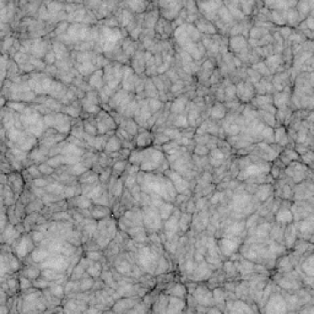
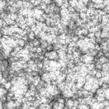
Model B	Model C
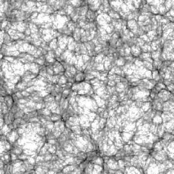
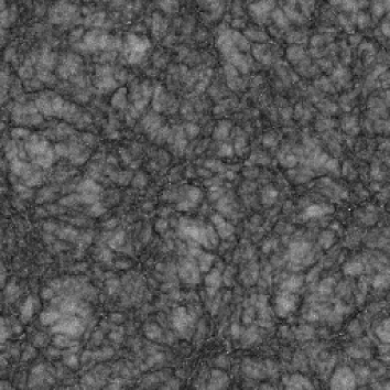
Model D	Model E

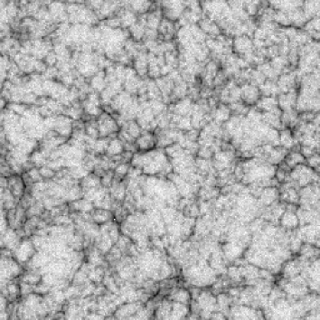
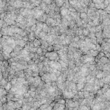
Figure 13: The projected density of ionized gas in a slice through the $\Lambda$CDM N-body simulation at $z=3$ shown as a greyscale image, with the densest regions being black. The slice shown has dimensions of $141.3\times 141.3\times 8.0h^{-1}$ Mpc. The total (i.e. ionized plus neutral) projected gas density is shown in the upper left hand panel. The remaining panels show the projected density of ionized gas in Models A-E.

Fig. 13 shows six slices through the N-body simulation. The top left slice shows the density of all gas (which is assumed to trace the dark matter), whilst the other slices show only the density of ionized gas. Model A shows particularly well the correlated nature of the ionizing sources (due to the fact that galaxies form in the high density regions of the dark matter), as the densest regions of the simulations are the ones which have become most highly ionized.

In Fig. 14 we show the filling factor in the N-body simulation for the fixed $f_{\rm esc,gas}$ model with different values of $f_{\rm esc,gas}$, for the case $f_{\rm clump}=f_{\rm clump}^{\rm(halos)}$. The filling factors calculated from the simulation are always less (for a given value of $f_{\rm esc,gas}$) than those calculated in §4.1 (see Fig. 10). This is because the simulation contains fewer low mass dark matter halos than predicted by the Press-Schechter theory, hence it contains fewer ionizing sources.

Figure 14: Filling factors as a function of redshift in the N-body simulation. Lines are plotted for the ‘fixed’ model with three different values of $f_{\rm esc,gas}$: 0.05 (solid line), 0.20 (dotted line) and 1.00 (short-dashed line).

6.2 CMB Fluctuations

The reionization of the IGM imprints secondary anisotropies on the CMB through Thomson scattering off free electrons (see, for example, ?; ?; ?). These anisotropies result from the spatially varying ionized fraction and from density and velocity variations in the ionized IGM. The calculation of these secondary effects involves correlation functions of density fluctuations and velocity fields which are easily determined in our models. To predict the form of these fluctuations, we first calculate the two-point correlations between ionized gas over the redshift range 3 to 18, assuming that gas in the IGM traces the dark matter density and velocity. To do this, we use the $256^{3}$ grid of ionization fractions, $x_{\rm e}$, described in §6.1. We determine in each grid cell the value of

$$\zeta=\left[{x_{\rm e}\left(1+\delta\right)\over\langle x_{\rm e}(1+\delta)\rangle}-1\right]v_{\rm los},$$ (10)

where $\delta$ is the dark matter overdensity in the cell, $v_{\rm los}$ is the component of the mean dark matter velocity in the cell along the line of sight to a distant observer, and the averaging of $x_{\rm e}(1+\delta)$ is over all cells in the simulation volume. The dark matter density and velocity in each cell are estimated by assigning the mass and velocity of each dark matter particle to the grid using a cloud-in-cell algorithm.

We then compute the correlation function

$$\xi_{\zeta\zeta}(r)=\langle\zeta({\bf x})\zeta({\bf x}+{\bf r})\rangle_{\bf x}.$$ (11)

This correlation function is all that is needed to determine the spectrum of fluctuations imprinted in the CMB by the reionization process. A detailed description of how this spectrum is computed is given in Appendix C.

Figure 15: The secondary CMB anisotropies generated measured from the simulation. The left hand panel shows the results for Model E, with a fixed gas escape fraction of 0.10. The solid line indicates a model in which unresolved halos are placed on ungrouped particles, whilst the dotted line shows a model with unresolved halos placed at random within the simulation volume. In the right-hand panel we show the results for $f_{\rm esc,gas}=1.00$ and with unresolved halos placed on ungrouped particles. The lines show the results from the five different models as indicated in the figure. In each case, the heavy solid line shows the primary anisotropies in this cosmology.

Figure 16: The effect of varying the escape fraction, $f_{\rm esc,gas}$, on the secondary CMB anisotropies. The curves shown are all computed using Model E, with unresolved halos placed on ungrouped particles. Gas escape fractions of 1.00, 0.70, 0.50, 0.20 and 0.05 are shown as indicated in the figure. The redshift of reionization for each model is also indicated. The heavy solid line shows the primary CMB anisotropies.

In Fig. 15 we show the secondary CMB anisotropies calculated as described above. The left-hand panel shows the results for Model E with a fixed gas escape fraction of 0.10, for the cases that unresolved halos are placed either on ungrouped particles (solid line) or at random in the simulation volume (dotted line). The clumping factor is $f_{\rm clump}=f_{\rm clump}^{\rm(halos)}$, as will be used for all models considered in this section. The particular choice of $f_{\rm clump}$ is not important for our conclusions about the CMB fluctuations, since we will consider different values of $f_{\rm esc,gas}$. The choice of placement scheme is seen to make little difference to the results, the two curves differing by $\lower 3.22916pt\hbox{$\sim$}\hbox to0.0pt{\hss\raise 1.1625pt\hbox{$<$}}10\%$ for $250<\ell<5000$, with the difference growing to 40% by $\ell=20000$. The size of the grid cell used in our calculation of the ionized gas correlation function corresponds to $\ell\approx 25000$ at $z=3$, and the turnover around $\ell=10^{4}$ is simply due to the cell size. As such, our method is unable to determine the form of the CMB fluctuations at higher $\ell$.

The right-hand panel of Fig. 15 shows the variations in our estimates of $C_{\ell}$ which arise from using the five Models A-E. Here the differences between the curves are larger, with Models B and C differing by a factor of $\approx 2.5$ at $\ell=10^{4}$. The amplitude of the curves is affected by the strength of the correlations present in each model (e.g. the “high density” model is the most strongly correlated and has the highest amplitude, whilst the “low density” model has the weakest correlations and hence the lowest amplitude). However, the shapes of the curves are all very similar.

Figure 16 examines the effect on the secondary anisotropies of varying the escape fraction $f_{\rm esc,gas}$. The trend is for increasing amplitude of anisotropy with increasing escape fraction (which results in a higher reionization redshift). If, however, we boost the number of photons produced by increasing $f_{\rm esc,gas}$ above 1 (this of course being unphysical, but a simple way of examining the effects of producing more ionizing photons), little further increase in amplitude is seen.

The form expected for the CMB anisotropies produced by patchy reionization has been calculated for a simple model by ?. In this model, reionization of the universe is assumed to begin at some redshift, $z_{\rm i}$, and is completed (i.e. the filling factor reaches unity) after a redshift interval $\delta z$. Sources are assumed to appear at random positions in space and to each ionize a spherical region of comoving radius $R$. Once such an ionized region has appeared it remains forever. In this model, the power $\ell^{2}C_{\ell}/2\pi$ is predicted to have the form of white noise at small $\ell$, since the ionized regions are uncorrelated.

We compare the simple model of ? with our own results in Fig. 16. Since in our model reionization has no well-defined starting redshift, and ionized regions span a range of sizes, we simply choose values of $R$, $z_{\rm i}$ and $\delta z$ in order to match the two models at the peak in the spectrum (even though the position of this peak in our results is an artifact of our simulation resolution, we simply wish to demonstrate here the difference in small $\ell$ slopes between our model and that of ?). The chosen values of $R=0.85h^{-1}$Mpc, $z_{\rm i}=11$ and $\delta z=5$ are all plausible for the ionization history and sizes of ionized regions seen in our model (the mean comoving size of regions ranging from $1.4h^{-1}$Mpc at $z=3$ to $0.2h^{-1}$Mpc at $z=18$). Note that ? calculate a somewhat different form for the anisotropy spectrum for this same model, in which the amplitude, $A$, is roughly half that found by ?, and the peak in the spectrum occurs at slightly higher $\ell$. Despite these differences both ? and ? agree upon the general form of the spectrum (sharp peak plus white noise at small $\ell$), and this is all we are interested in here.

The $C_{\ell}$ declines much more rapidly as $\ell\rightarrow 0$ in the ? model than in ours. Note that Model D, the random sphere model, also shows the same behaviour as our other models, indicating that it is not the correlated positions of the ionizing sources in our model which produce the excess power at small $\ell$. If we force all halos in our model to have equal ionized volumes surrounding them, whilst retaining the same total filling factor, we find that the excess power above the white noise spectrum at small $\ell$ remains, so neither is the excess due to the range of ionizing front radii, $R$, present in our model. This excess power can therefore be seen to be due to the correlations in gas density and velocity induced by gravity. In fact, if we repeat our calculations but ignore correlations in the gas density field (i.e. we set $\delta=0$ everywhere) we find a CMB spectrum which has a slope for small $\ell$ which is much closer to the ? white-noise slope, and which has an amplitude over five times lower than when density correlations are included. The remaining differences between our model and that of ? in this case are due to the correlated nature of ionized regions in our model.

Figure 17: The effect of varying $\Omega_{\rm b}$ on the secondary CMB anisotropies. The curves shown are all computed using Model E, with unresolved halos placed on ungrouped particles and a gas escape fraction of 1.0. The solid line shows $\Omega_{\rm b}=0.02$ whilst the dotted line shows $\Omega_{\rm b}=0.04$ (Model 1 in Table 2). The heavy solid line shows the primary CMB anisotropies.

The amplitude of the secondary anisotropies also depends upon the assumed value of $\Omega_{\rm b}$ (as this determines the optical depth for electron scattering). The preferred value for our galaxy formation model of $\Omega_{\rm b}=0.02$ is relatively low compared to estimates based on light element abundances and big bang nucleosynthesis. Fig. 17 shows the effect of increasing $\Omega_{\rm b}$ to 0.04. If the evolution of the ionized regions were the same in both models, we would expect the amplitude to increase by a factor of four (since it is proportional to the square of the baryon density). The evolution of ionized regions is actually quite similar in the two cases, and so the factor of four increase is seen. With this higher value of $\Omega_{\rm b}$, the secondary anisotropies due to patchy reionization would be potentially detectable above $\ell\sim 3000$.

We note that a similar approach to computing the spectrum of secondary anisotropies due to patchy reionization has been taken by ?. Using a different model of galaxy formation, ? grow spherical ionization fronts around dark matter halos identified in an N-body simulation, and from these they estimate the spectrum of CMB anisotropies produced. The simulations employed by ? have higher resolution (but much smaller volume) than the GIF simulations used in our work. ? therefore do not have the problem of locating unresolved halos in their simulation, but their calculation of secondary anisotropies is restricted to smaller angular scales (roughly $5\times 10^{3}\lower 3.22916pt\hbox{$\sim$}\hbox to0.0pt{\hss\raise 1.1625pt\hbox{$<$}}\ell\lower 3.22916pt\hbox{$\sim$}\hbox to0.0pt{\hss\raise 1.1625pt\hbox{$<$}}2\times 10^{5}$) compared to ours. Furthermore, ? make some approximations in calculating the anisotropies which we do not, ignoring variations in the total IGM density, and assuming that the ionized fraction is completely uncorrelated with the velocity field. ? consider only a single model for reionizing the simulation volume. As we have shown, our five toy models for the distribution of ionized regions lead to factors of 2–3 difference in the secondary anisotropy amplitudes, indicating that the results are not very sensitive to the model adopted for the distribution of ionized regions or to the treatment of unresolved halos in the simulation. ? carried out their calculations in a different cosmology to ours, also with a different value of $\Omega_{\rm b}$, but once these differences are taken into account, their results seem reasonably consistent with ours.

7 Discussion and Conclusions

We have outlined an approach to studying the reionization of the universe by the radiation from stars in high redshift galaxies. We have focussed on the reionization of hydrogen, but the approach can be generalised to study helium reionization (e.g. ?), and also to include radiation from quasars. Our main conclusions are:

(i) Using a model of galaxy formation constrained by several observations of the local galaxy population, enough ionizing photons are produced to reionize the universe by $z=11.7$. This assumes that all ionizing photons escape from the galaxies they originate in, and that the density of the IGM is uniform. Reionization is delayed until $z\approx 10.9$ in the case of a clumped IGM, in which gas falls into halos with virial temperatures exceeding $10^{4}$K. Galaxies can reionize such a clumped IGM by $z=5$ providing that, on average, at least 4% of ionizing photons can escape from the galaxies where they are produced. In the case of a uniform IGM, an escape fraction of only 1.4% is sufficient to reionize by $z=5$.

Using a physical model for the escape of ionizing radiation from galaxies, in which photons escape through “Hii chimneys” ionized in the gas layers in galaxy disks (?, hereafter DS94), we predict reionization by $z=6.1$ for a uniform IGM or by $z=4.5$ for a clumped IGM. Models which assume that all the gas in galaxy disks remains neutral are unable to reionize even a uniform IGM by $z=0$. Using alternative estimates of the IGM clumping factor from ? or ?, we find reionization redshifts comparable with those found using our own clumping model, i.e. in the range $z=$ 4.5–5.0 with the DS94 model for the escape fraction.

(ii) Once the ionizing escape fraction and IGM clumping factor have been specified, our estimates for the filling factor of ionized gas in the IGM are reasonably robust, providing that we consider only models which are successful in matching the H$\alpha$ luminosity function of galaxies at $z=0$. By far the greatest remaining influences on the ionized filling factor come from the value of the baryon fraction $\Omega_{\rm b}$ and the prescription for feedback from supernovae. However, we have shown that altering these parameters also produces large changes in the $z=0$ H$\alpha$ luminosity function.

(iii) We combined our model for reionization with N-body simulations of the dark matter distribution in order to predict the spectrum of secondary anisotropies imprinted on the CMB by the process of reionization. The shape of this spectrum is almost independent of the assumptions about reionization, but the amplitude depends on the spatial distribution of the ionized regions, the redshift at which reionization occurs and the baryon fraction. We find considerably more power in the anisotropy spectrum at small $\ell$ than predicted by models which do not account for the large-scale correlations in the gas density and velocity produced by gravity. Despite the uncertainty in the spatial distribution of ionized regions, we are able to determine the amplitude of this spectrum to within a factor of three for a given $\Omega_{\rm b}$ (the amplitude being proportional to $\Omega_{\rm b}^{2}$). The results found by ? using a similar technique are reasonably consistent with ours, once differences in $\Omega_{\rm b}$ and other cosmological parameters are allowed for.

Detection of these secondary anisotropies, which would constrain the reionization history of the Universe, would require fractional temperature fluctuations of $\sim 10^{-7}$ to be measured on angular scales smaller than several arcminutes. Although the Planck and MAP space missions are unlikely to have sufficient sensitivity to observe such anisotropies, the Atacama Large Millimeter Array is expected to be able to measure temperature fluctuations of the level predicted at $\ell\sim 10^{4}$ in a ten hour integration.

Previous studies of reionization have either used an approach similar to our own, i.e. employing some type of analytical or semi-analytical model (e.g. ?; ?; ?; ?), or else have used direct hydrodynamical simulations (e.g. ?). While the latter technique can in principle follow the detailed processes of galaxy formation, gas dynamics and radiative transfer, in practice the resolutions attainable at present do not allow such simulations to resolve the small scales relevant to this problem. Furthermore, the implementation of star formation and feedback in such models is far from straightforward.

There are two main uncertainties in our approach, as in most others: the fraction $f_{\rm esc}$ of ionizing photons that escape from galaxies, and the clumping factor $f_{\rm clump}$ of gas in the IGM. Future progress depends on improving estimates of the effects of clumping using larger gas dynamical simulations, on better modelling of the escape of ionizing photons from galaxies, and on better understanding of star formation and supernova feedback in high redshift objects.

Appendix A Calculation of the escaping fraction

A.1 Escaping fraction in the DS94 model: Stars in mid-plane

In the model of ?, hereafter DS94, ionizing photons escape from galactic disks through “Hii chimneys”, which are holes in the neutral gas layer ionized by OB associations. The OB associations are assumed to lie in the disk mid-plane, and to have a distribution of ionizing luminosities ${\rm d}N/{\rm d}S\propto S^{-2}$ for $S_{1}<S<S_{2}$, $({\rm d}N/{\rm d}S){\rm d}S$ being the number of associations with luminosities in the range $S$ to $S+{\rm d}S$ (?). The gas is assumed to have a Gaussian vertical distribution with scaleheight $h_{\mathrm{z}}$. The fraction of Lyc photons escaping through chimneys on both sides of the disk at radius $r$ is (?, eqn. 24)

$$f_{\rm esc,gas}=\left\{\begin{array}[]{ll}0&\hbox{if }S_{\rm m}\geq S_{2}\\ \left.\left[\ln\left({S_{2}\over S_{\mathrm{m}}}\right)+{9\over 2}\left({S_{\rm m}\over S_{2}}\right)^{1/3}-{S_{\rm m}\over 2S_{2}}-4\right]\right/\ln\left({S_{2}\over S_{1}}\right)&\hbox{if }S_{1}\leq S_{\rm m}<S_{2}\\ 1+\left.\left[{9\over 2}\left\{\left({S_{\rm m}\over S_{2}}\right)^{1/3}-\left({S_{\rm m}\over S_{1}}\right)^{1/3}\right\}-{1\over 2}\left\{{S_{\rm m}\over S_{2}}-{S_{\rm m}\over S_{1}}\right\}\right]\right/\ln\left({S_{2}\over S_{1}}\right)&\hbox{if }S_{\rm m}<S_{1},\end{array}\right.$$ (12)

where $S_{\mathrm{m}}$ is defined as

$$S_{\rm m}(r)=\pi^{3/2}n_{0}^{2}\exp\left(-2r/r_{\rm disk}\right)h_{\mathrm{z}}^{3}\alpha_{\mathrm{H}}^{(2)},$$ (13)

Here $\alpha_{\mathrm{H}}^{(2)}$ is the recombination coefficient for hydrogen for recombinations to all energy levels except the first, and we have assumed an exponential disk with radial scalelength $r_{\rm disk}$, so that the hydrogen gas density is

$$n(r,z)=n_{0}\exp(-r/r_{\rm disk}-z^{2}/2h_{\rm z}^{2}),$$ (14)

$r$ and $z$ being the usual cylindrical polar coordinates.

Since $S_{\rm m}$ varies throughout the galactic disk we average the escape fraction over the entire disk, assuming that the local rate of star formation is proportional to the column density of the disk (?; ?) and that $h_{\rm z}$ is constant with radius.

The fraction of all ionizing photons produced by the galaxy which can escape into the IGM is then given by,

$$f_{\rm esc,gas}=\left\{\begin{array}[]{ll}\left.\left[\left\{{352\over 225}-{4\over 15}\ln\left({S_{2}\over S_{\rm m}^{0}}\right)\right\}\left({S_{2}\over S_{\rm m}^{0}}\right)^{1/2}-\left\{{352\over 225}-{4\over 15}\ln\left({S_{1}\over S_{\rm m}^{0}}\right)\right\}\left({S_{1}\over S_{\rm m}^{0}}\right)^{1/2}\right]\right/\ln\left({S_{2}\over S_{1}}\right)&\hbox{if }S_{\rm m}^{0}\geq S_{2}\\ \left.\left[\left\{{4\over 15}\ln\left({S_{1}\over S_{\rm m}^{0}}\right)-{352\over 225}\right\}\left({S_{1}\over S_{\rm m}^{0}}\right)^{1/2}-{1\over 18}{S_{\rm m}^{0}\over S_{2}}+{81\over 50}\left({S_{\rm m}^{0}\over S_{2}}\right)^{1/3}+\ln\left({S_{2}\over S_{\rm m}^{0}}\right)\right]\right/\ln\left({S_{2}\over S_{1}}\right)&\hbox{if }S_{1}\leq S_{\rm m}^{0}<S_{2}\\ 1+\left.\left[{81\over 50}\left\{\left({S_{\rm m}^{0}\over S_{2}}\right)^{1/3}-\left({S_{\rm m}^{0}\over S_{1}}\right)^{1/3}\right\}-{1\over 18}\left\{{S_{\rm m}^{0}\over S_{2}}-{S_{\rm m}^{0}\over S_{1}}\right\}\right]\right/\ln\left({S_{2}\over S_{1}}\right)&\hbox{if }S_{\rm m}^{0}<S_{1},\end{array}\right.$$ (15)

where $S^{0}_{\rm m}$ is the value of $S_{\rm m}$ calculated for $r=0$. In Figure 18 we show this average escape fraction as a function of the ratio $S^{0}_{\mathrm{m}}/S_{2}$ for $S_{2}/S_{1}=1000$.

Figure 18: The average escape fraction for a galactic disk in the DS94 model with OB associations in the disk mid-plane (solid line) and distributed as the cold gas (dashed line). Both models assume $S_{2}/S_{1}=1000$. The dotted line (visible just above the solid line at small values of $S_{\rm m}^{0}/S_{2}$) shows the effects of accounting for radial variations in the gas density in the model where OB associations are distributed as the gas. This line only differs noticeably from the dashed line at the lowest values of $S^{0}_{\mathrm{m}}/S_{2}$.

Our model of galaxy formation calculates the radial scale length of each galaxy’s disk and also the mass of cold gas present in that disk, and we assume that $h_{\mathrm{z}}/r_{\rm disk}$ is constant. We can therefore determine $n_{0}$ and the ratios $S^{0}_{\rm m}/S_{2}$ and $S^{0}_{\rm m}/S_{1}$. Hence $f_{\rm esc,gas}$ can be found using eqn. (15).

A.2 Escaping fraction in DS94 model: Stars tracing gas

In the DS94 model OB associations are assumed to lie in the midplane of the galaxy disk. If instead OB associations are spread throughout the gas layer, having the same vertical distribution as the cold gas, then the resulting escape fraction will be higher than that in the DS94 model. We assume the same density profile as before, given by eqn.(14). Consider an OB association emitting $S$ ionizing photons per second, at position $(r,z)$ in the disk. We make the assumption (as did DS94) that the radial variations in density can be ignored for calculating the escape fraction at radius $r$ (which will be a valid assumption provided the size of the Hii region formed is much less than $r_{\rm disk}$). In order for any photons emitted into a cone of solid angle ${\rm d}\Omega$ which makes an angle $\theta$ with the $z$-axis to escape the galaxy, the emission rate of photons into this cone must exceed the total recombination rate in the cone. This occurs for an ionizing luminosity $S_{\rm req}(\theta)$, where,

$$S_{\rm req}(\theta){{\rm d}\Omega\over 4\pi}=n_{0}^{2}\alpha_{\rm H}^{(2)}\exp\left(-2{r\over r_{\rm disk}}\right)\int_{0}^{\infty}l^{2}\exp\left(-{(z+l\cos\theta)^{2}\over h_{\rm z}^{2}}\right){\rm d}l{\rm d}\Omega,$$ (16)

which can be written as $S_{\rm req}^{\pm}(\theta)=\pm S_{\rm req}^{0,\pm}/\cos^{3}\theta$ ($S_{\rm req}^{+}$ is the solution for $\cos\theta>0$ and $S_{\rm req}^{-}$ is the solution for $\cos\theta<0$), where

$$S_{\rm req}^{0,\pm}=S_{\rm m}^{0}{\rm e}^{-2r/r_{\rm disk}}\left\{\left[1\mp{\rm erf}\left({z\over h_{\rm z}}\right)\right]\left(1+{2z^{2}\over h_{\rm z}^{2}}\right)-{2\over\sqrt{\pi}}{z\over h_{\rm z}}\exp\left(-{z^{2}\over h_{\rm z}^{2}}\right)\right\}.$$ (17)

This defines two critical angles, $\cos\theta_{\rm c}^{\pm}(S)=\pm(S_{\rm req}^{0,\pm}/S)^{1/3}$, such that photons can escape the galaxy only if $\theta<\theta_{\rm c}^{+}(S)$ or $\theta>\theta_{\rm c}^{-}(S)$.

The total escaping fraction from this OB association is then given by,

$$f_{\rm esc,gas}(S) = {1\over 2S}\left[\int_{\cos\theta_{\rm c}^{+}}^{1}\left[S-S_{\rm req}^{+}(\theta)\right]\>{\rm d}(\cos\theta)+\int^{\cos\theta_{\rm c}^{-}}_{-1}\left[S-S_{\rm req}^{-}(\theta)\right]\>{\rm d}(\cos\theta)\right]$$ (18)

$$f_{\rm esc,gas}(S) = 1-{3\over 4}\left({S_{\rm req}^{0,+}\over S}\right)^{1/3}-{3\over 4}\left({S_{\rm req}^{0,-}\over S}\right)^{1/3}+{S_{\rm req}^{0,+}\over 4S}+{S_{\rm req}^{0,-}\over 4S}.$$ (19)

Averaging this escape fraction over the assumed OB association luminosity function then gives a mean escape fraction of

$$f_{\rm esc,gas}=\left\{\begin{array}[]{ll}0&\hbox{if }S_{2}>S_{\rm m}^{0}{\rm e}^{-2r/r_{\rm disk}}\\ \begin{array}[]{r}\left.\left[{1\over 2}\ln\left({S_{2}^{2}\over S_{\rm req}^{0,+}S_{\rm req}^{0,-}}\right)+{9\over 4}\left\{\left({S_{\rm req}^{0,+}\over S_{2}}\right)^{1/3}+\left({S_{\rm req}^{0,-}\over S_{2}}\right)^{1/3}-2\right\}\right.\right.\\ \left.\left.-{1\over 4}\left\{{S_{\rm req}^{0,+}\over S_{2}}+{S_{\rm req}^{0,-}\over S_{2}}-2\right\}\right]\right/\ln\left({S_{2}\over S_{1}}\right)\end{array}&\hbox{if }S_{1}<S_{\rm m}^{0}{\rm e}^{-2r/r_{\rm disk}}\leq S_{2}\\ \begin{array}[]{r}1+\left.\left[{9\over 4}\left\{\left({S_{\rm req}^{0,+}\over S_{2}}\right)^{\frac{1}{3}}-\left({S_{\rm req}^{0,+}\over S_{1}}\right)^{\frac{1}{3}}+\left({S_{\rm req}^{0,-}\over S_{2}}\right)^{\frac{1}{3}}-\left({S_{\rm req}^{0,-}\over S_{1}}\right)^{\frac{1}{3}}\right\}\right.\right.\\ \left.\left.-{1\over 4}\left\{{S_{\rm req}^{0,+}\over S_{2}}-{S_{\rm req}^{0,+}\over S_{1}}+{S_{\rm req}^{0,-}\over S_{2}}-{S_{\rm req}^{0,-}\over S_{1}}\right\}\right]\right/\ln\left({S_{2}\over S_{1}}\right)\end{array}&\hbox{if }S_{\rm m}^{0}{\rm e}^{-2r/r_{\rm disk}}\leq S_{1}\end{array}\right.$$ (20)

This expression is then averaged over the galaxy disk, assuming a star formation rate proportional to the local gas density, to derive the mean escaping fraction for the entire galaxy. This must be done numerically

Although we have ignored radial variations in the density of the gas when computing the escaping fraction from a single OB association, we find by numerical solution that these variations make only a very small difference to the value of $f_{\rm esc,gas}$, and then only for small $S_{\rm m}^{0}/S_{2}$ (see Fig. 18).

A.3 Escaping fraction in the DSGN98 model

In the model of ?, DSGN98 the stars producing the Lyman continuum photons are assumed to be uniformly mixed with the gas in the galaxy, which is distributed in an exponential disk. All of the hydrogen in the galaxy is assumed to be in the form of Hi, allowing the optical depth for ionizing photons to be calculated.

We have calculated the escaping fraction in this model exactly, using the density profile given by eqn. (14). As in the case of the DS94 model with stars mixed uniformly with the gas, we begin by finding the escaping fraction as a function of position $(r_{0},z_{0})$ and line of sight $(\theta,\phi)$. For the DSGN98 model we therefore find the total optical depth in neutral hydrogen along the line of sight, which is

$$\tau_{(}r_{0},z_{0},\theta,\phi)=\sigma_{\rm H{\sc i}}\int^{\infty}_{0}n(r,z){\rm d}l,$$ (21)

where $\sigma_{\rm H{\sc i}}=6.3\times 10^{-18}{\rm cm}^{-2}$ is the cross-section for hydrogen ionization at 912Å. The quantity $\exp(-\tau)$ is then averaged over all $r_{0}$, $z_{0}$, $\theta$ and $\phi$, assuming that the star formation rate is proportional to the local gas density, to obtain the final escaping fraction. The average escape fraction for the entire galaxy depends only on the quantity $\tau_{0}=n_{0}r_{\rm disk}\sigma_{\rm H}$ for a given value of $h_{\rm z}/r_{\rm disk}$, and is shown in Fig. 19 for $h_{\rm z}/r_{\rm disk}=0.1$.

Figure 19: Mean escape fraction for a galaxy disk in the DSGN98 model as a function of $\tau_{0}$.

A.4 Escaping fraction in starbursts

In the case of a burst of star formation triggered by a major merger, we use the same $f_{\rm esc,gas}$ as for quiescent star formation in the the case where $f_{\rm esc,gas}$ is assumed fixed, but in the DS94 and DSGN98 models we estimate the escape fraction by assuming the burst has an approximately spherical geometry, throughout which star formation proceeds uniformly. We assume a sphere of uniform hydrogen number density, $n$, given by

$$n={3M_{\rm gas}\over 4\pi r_{\rm burst}^{3}1.4{\rm m}_{\rm H}},$$ (22)

where $M_{\rm gas}$ is the mass of cold gas in the burst, $r_{\rm burst}$ is the radius of the region in which the burst occurs, and ${\rm m}_{\rm H}$ is the mass of a hydrogen atom. The factor of 1.4 accounts for the presence of helium in the gas. We assume also that photons escape only from an outer shell of thickness $l$, within which the optical depth is less than 1. Therefore,

$$nl\sigma_{\rm H{\sc i}}\approx 1,$$ (23)

where $\sigma_{\rm H{\sc i}}$ is the cross section for hydrogen ionization. The escape fraction is simply the fraction of the sphere’s volume in this shell, i.e.

$$f_{\rm esc,gas}\approx{4\pi r_{\rm burst}^{2}l\over 4\pi/3r_{\rm burst}^{3}}.$$ (24)

Substituting for $l$ then gives

$$f_{\rm esc,gas} = {3\over r_{\rm burst}n\sigma_{\rm H{\sc i}}}$$ (25)

$$= {4\pi r_{\rm burst}^{2}1.4{\rm m}_{\rm H}\over M_{\rm gas}\sigma_{\rm H{\sc i}}}.$$

We take $r_{\rm burst}$ to be equal to $0.1r_{\rm bulge}$ where $r_{\rm bulge}$ is the half-mass radius of the bulge formed by the merger. This choice is motivated by observational fact which shows that starburst activity is usually confined to the nuclear region, the size of which is much smaller than that of the galaxy as a whole (e.g. ? and references therein). ? have carried out more elaborate calculations of escaping fractions from spherical galaxies. However, their results are applicable to gas in hydrostatic equilibrium with an NFW dark matter profile and so are not well suited to the case of starbursts.

The star formation rate in the burst is assumed to decline exponentially, with an e-folding time equal to $f_{\rm dyn}$ times the bulge dynamical time. Unless noted otherwise, we assume $f_{\rm dyn}=1$ in all models. As the burst proceeds the mass of cold gas present, $M_{\rm gas}$, declines as it is turned into stars. The escape fraction, $f_{\rm esc,gas}$, therefore increases during the burst, reaching unity as the amount of gas present drops to zero. However, as the star formation rate is declining exponentially during the burst only a small fraction of photons are produced whilst $f_{\rm esc,gas}$ is high.

Appendix B Calculation of Clumping Factor

To estimate the clumping factor of the photoionized IGM, we make the simplifying assumption that gas in the universe can be split into three components — that which has fallen into dark matter halos and is collisionally ionized or is part of a galaxy, that which has fallen into dark matter halos and is not collisionally ionized, and that which has remained outside halos and is smoothly distributed. The first component makes no contribution to the clumping factor. We define the clumping factor as

$$f_{\rm clump}={\langle\rho_{\rm IGM}^{2}\rangle\over\bar{\rho}_{\rm IGM}^{2}}={\langle\rho_{\rm IGM}^{2}\rangle\over f_{\rm IGM}^{2}\bar{\rho}^{2}},$$ (26)

where $\rho_{\rm IGM}$ is the IGM gas density at any point in the universe (i.e. it does not include contributions from collisionally ionized gas or galaxies), $\bar{\rho}_{\rm IGM}=f_{\rm IGM}\bar{\rho}$ is the mean density of gas in the IGM and $\bar{\rho}$ is the mean density of all gas in the universe (here $f_{\rm IGM}$ is the fraction of the total mass of gas in the universe which resides in the IGM, as defined in §2.2).

Let $f_{\rm m,clumped}$ be the fraction of mass in halos above the Jeans halo mass, $M_{\rm J}$, as calculated from the Press-Schechter mass function for example. These halos occupy a fraction of the volume of the universe given by $f_{\rm v,clumped}=f_{\rm m,clumped}/\Delta_{\rm vir}$. Here, $\Delta_{\rm vir}$ is the mean density within the virial radius of a halo in units of the mean density of the Universe. The smooth component of gas is assumed to uniformly fill the region outside halos with $M>M_{\rm J}$, and so has density

$$\rho_{\rm smooth}=\bar{\rho}f_{\rm m,smooth}/f_{\rm v,smooth},$$ (27)

where $f_{\rm m,smooth}=1-f_{\rm m,clumped}$ is the mass fraction of gas in this smooth component, and $f_{\rm v,smooth}=1-f_{\rm v,clumped}$ is the fraction of the volume of the universe that it occupies.

Consider next the non-collisionally ionized gas in a single dark matter halo. Averaging over the volume of this one halo we obtain

$$\langle\rho_{\rm clumped}^{2}\rangle=f_{\rm int}(1-f_{\rm gal})^{2}(1-x_{\rm H})^{2}\Delta_{\rm vir}^{2}\bar{\rho}^{2},$$ (28)

where $f_{\rm gal}$ is the fraction of the baryons which have become part of galaxies within the halo, $x_{\rm H}$ is the ionized fraction for the hydrogen in the halo gas assuming collisional ionization equilibrium (which we take from the calculations of ?), and $f_{\rm int}$ is a factor of order unity which depends on the shape of the halo gas density profile and is given by

$$f_{\rm int}={\int_{0}^{r_{\rm vir}}\rho^{2}(r)r^{2}{\rm d}r\over\int_{0}^{r_{\rm vir}}\bar{\rho}_{int}^{2}r^{2}{\rm d}r}.$$ (29)

Here $r_{\rm vir}$ is the virial radius of the halo, $\rho(r)$ is the density profile of the diffuse gas in the halo, and $\bar{\rho}_{int}$ is the mean density of this gas within the virial radius. We ignore any dependence of the density profile of the gas in the halo on the fraction which has cooled to form galaxies. Our results should be insensitive to this assumption, as $f_{\rm gal}\ll 1$ in halos where $x_{\rm H}$ is significantly less than unity.

To find the contribution of gas in halos to the clumping factor, we integrate the above expression over all halos more massive than $M_{\rm J}$, weighting by the volume for each halo. Adding the contribution from the smooth component, we then obtain

$$f_{\rm clump}={f_{\rm m,smooth}^{2}\over f_{\rm v,smooth}f_{\rm IGM}^{2}}+{f_{\rm int}\Delta_{\rm vir}\over f_{\rm IGM}^{2}}\int_{M_{\rm J}}^{\infty}\langle(1-f_{\rm gal})^{2}\rangle(1-x_{\rm H})^{2}{M_{\rm halo}\over\rho_{\rm c}\Omega_{0}}{{\rm d}n\over{\rm d}M_{\rm halo}}{\rm d}M_{\rm halo},$$ (30)

where we have used that fact that the comoving volume of a dark matter halo of mass $M_{\rm halo}$ is $M_{\rm halo}/(\Delta_{\rm vir}\Omega_{0}\rho_{\rm c})$ ($\rho_{\rm c}$ being the critical density of the universe at $z=0$). Here $\langle(1-f_{\rm gal})^{2}\rangle$ is averaged over all halos of mass $M_{\rm halo}$ in our model of galaxy formation.

We determine $M_{\rm J}$ by finding the mass of a dark matter halo which has a potential well deep enough that it can just hold onto reionized gas. This gives us the minimum mass halo within which gas collects. For the halo to just retain its gas,

$${{\rm d}P\over{\rm d}r}={{\rm G}M_{\rm J}\over r_{\rm vir}^{2}}\rho(r_{\rm vir}),$$ (31)

where $r_{\rm vir}$ is the virial radius of the halo and $P$ is the gas pressure. We approximate this as

$${P\over r_{\rm vir}}\approx{{\rm G}M_{\rm J}\over r_{\rm vir}^{2}}\rho(r_{\rm vir}),$$ (32)

and using the ideal gas law this becomes

$${{\rm k}_{\rm B}T\over\mu{\rm m}_{\rm H}}\approx{{\rm G}M_{\rm J}\over r_{\rm vir}}={4\pi\over 3}{\rm G}r^{2}_{\rm vir}\rho_{\rm c}\Omega_{0}\Delta_{\rm vir}(1+z)^{3},$$ (33)

where we have used the relation $M_{\rm J}=4\pi\rho_{\rm c}\Omega_{0}(1+z)^{3}\Delta_{\rm vir}r_{\rm vir}^{3}/3$. The virial radius is therefore

$$r_{\rm vir}=\left({3\over 4\pi}{{\rm k}_{\rm B}T\over{\rm G}\mu{\rm m_{\rm H}}\rho_{\rm c}\Omega_{0}\Delta_{\rm vir}}\right)^{1/2}(1+z)^{-3/2},$$ (34)

and the minimum halo mass in which gas is retained is

$$M_{\rm J}={4\pi\over 3}\rho_{\rm c}(1+z)^{3}\Omega_{0}\Delta_{\rm vir}r_{\rm vir}^{3}.$$ (35)

We evaluate $f_{\rm int}$ for the case of an isothermal profile with core radius $r_{\rm c}$:

$$\rho(r)\propto{1\over r^{2}+r_{\rm c}^{2}}.$$ (36)

The simulations of galaxy clusters by ? and ? show that the gas density profile is well described by this form. Substituting this in eqn. (29), we find

$$f_{\rm int}={1\over 6}\left({r_{\rm vir}\over r_{\rm c}}\right)^{3}\left[{r_{\rm vir}\over r_{\rm c}}-\arctan{r_{\rm vir}\over r_{\rm c}}\right]^{-2}\left[\arctan{r_{\rm vir}\over r_{\rm c}}-{r_{\rm vir}\over r_{\rm c}}\left(1+{r_{\rm vir}^{2}\over r_{\rm c}^{2}}\right)^{-1}\right].$$ (37)

For a typical value of $r_{\rm vir}/r_{\rm c}=10$, we therefore find $f_{\rm int}=3.14$.

Appendix C The Spectrum of CMB Secondary Anisotropies

In this paper, we concentrate on the kinematic Sunyaev-Zel’dovich effect which is induced by the peculiar motions (deviations from pure Hubble flow) of free electrons in ionized regions (?; ?). There exist other secondary sources of CMB anisotropies. However, on angular scales smaller than a few arc-minutes, the kinematic Sunyaev-Zel’dovich effect is likely to provide a dominant contribution. For example, it is known that the temperature anisotropies caused by non-linear growth of density perturbations, which are often referred to as the Rees-Sciama effect or integrated Sachs-Wolfe effect, are of order $10^{-7}$ or less (?). These anisotropies depend on the the baryon bulk physical peculiar velocity, ${\bf v}$, and the number density of free electrons, $n_{\mathrm{e}}$. In our calculations of the anisotropies we assume that the $\bf v$ is equal to the bulk velocity of the dark matter and that $n_{\rm e}$ in ionized regions is proportional to the dark matter density.

The temperature anisotropy $\Theta(\mbox{\boldmath$\gamma$})=\frac{\Delta T}{T}$ observed in a given line of sight direction $\gamma$ is (e.g. ?)

$$\Theta(\mbox{\boldmath$\gamma$},\eta_{0})=-\int_{\eta_{\rm rec}}^{\eta_{0}}\frac{{\rm d}\eta}{(1+z)}\gamma_{i}v_{\rm B}^{i}{\dot{\tau}},$$ (38)

where $\eta\equiv\int(1+z){\rm d}t$ is conformal time with its values at recombination and present denoted, respectively, by $\eta_{\rm rec}$ and $\eta_{0}$. In eqn. (38) we have assumed an optically thin universe. In an optically thick universe these temperature fluctuations are damped by a factor ${\rm e}^{-\tau}$, where the optical depth is $\tau=\int{\mathrm{d}}\eta\sigma_{\mathrm{T}}n_{\mathrm{e}}/(1+z)$, where $\sigma_{\rm T}$ is the cross section for Thomson scattering. If the universe became instantaneously fully ionized after some redshift $z_{\rm i}$, the relation between the optical depth $\tau(\eta_{\rm i},\eta_{0})$ and $z_{\rm i}$ is approximately obtained as $z_{\rm i}=100\Omega_{0}\left(0.025/\Omega_{\rm b}h\right)^{2/3}\tau^{1/3}$. Therefore, if the reionization takes place at $z\ll 100\Omega_{0}\left(0.025/\Omega_{\rm b}h\right)^{2/3}$, as is the case in our reionization model, then the damping factor can be neglected.

The usual procedure to obtain the angular correlation function of temperature anisotropies in eqn. (38) is by means of Limber’s equation in Fourier space (see for example ?). However, in this paper, we work in real space since we have the two point correlation functions of density and velocity fields directly measured in real space from N-body simulations.

The temperature angular correlation $C(\theta)$ can be written as

$$C(\theta)=\sigma^{2}_{\rm T}\int_{{\eta_{\mathrm{r}ec}}}^{\eta_{0}}{\rm d}\eta\int_{{\eta_{\rm rec}}}^{\eta_{0}}{\rm d}\eta^{\prime}\gamma_{i}\gamma_{j}^{\prime}<v^{i}({\bf x},\eta)v^{j}({\bf x}^{\prime},\eta^{\prime}){n_{\rm e}({\bf x},\eta)}{n_{\rm e}({\bf x}^{\prime},\eta^{\prime})}>,$$ (39)

where $\gamma_{i}\gamma^{\prime i}=\cos\theta$, and, $\bf x$ and ${\bf x}^{\prime}$ refer, respectively, to comoving coordinates in the past light geodesics in the directions $\gamma$ and $\gamma^{\prime}$ at $\eta$ and $\eta^{\prime}$. We write $n_{\mathrm{e}}$ terms of density fluctuations $\delta$ as

$$n_{\rm e}({\bf x},\eta)=\bar{n}_{\rm e}(\eta)x_{\rm e}({\bf x},\eta)\left[1+\delta({\bf x},\eta)\right],$$ (40)

where $\bar{n}_{\rm e}(\eta)$ is the mean total (free and bound) electron number density at time $\eta$, and $x_{\rm e}({\bf x})$, the ionization fraction, is unity in ionized regions and zero otherwise. The correlation lengths of velocity and density fields are small compared to the Hubble radius so that we can approximate $n_{\mathrm{e}}({\bf x}^{\prime},\eta^{\prime})=n_{\mathrm{e}}({\bf x}^{\prime},\eta)$ and similarly for the $v$, in eqn. (39).

$$\zeta=\left[{x_{\rm e}\left(1+\delta\right)\over\langle x_{\rm e}(1+\delta)\rangle}-1\right]v_{\rm los},$$ (41)

where $v_{\rm los}=\gamma_{i}v^{i}$ is the velocity component in the direction $\gamma$. Therefore $C(\theta)$ can be written in terms of the velocity correlation function $\xi_{vv}(y)\equiv<v_{\rm los}({\bf x})v_{\rm los}({\bf x}+{\bf y})>$ and the density-velocity correlation function $\xi_{\zeta\zeta}(y)\equiv<\zeta({\bf x})\zeta({\bf x}+{\bf y})>$, both evaluated for fields at the same $\eta$.

$$C(\theta)=\sigma_{\rm T}^{2}\int_{\eta_{\rm rec}}^{\eta_{0}}{{\rm d}\eta\over 1+z}\int_{\eta_{\rm rec}}^{\eta_{0}}{{\rm d}\eta^{\prime}\over 1+z^{\prime}}\bar{n}_{\rm e}(\eta)\bar{n}_{\rm e}(\eta^{\prime})\langle x_{\rm e}(1+\delta)\rangle^{2}\left[\xi_{\zeta\zeta}(|{\bf x}^{\prime}-{\bf x}|)+\xi_{vv}(|{\bf x}^{\prime}-{\bf x}|)+\langle\zeta({\bf x})v_{\rm los}({\bf x}^{\prime})+\zeta({\bf x}^{\prime})v_{\rm los}({\bf x})\rangle\right].$$ (42)

The dominant contribution to $C(\theta)$ is from the term involving $\xi_{\zeta\zeta}$. The integration over $\xi_{vv}$ yields to phase cancellation (?; ?; ?). The last term in the integrand also has negligible contribution. We have checked that the dominant term produces at least an order of magnitude larger anisotropies than the other terms.

In flat space we use the triangle relation, $|{\bf x}^{\prime}-{\bf x}|^{2}=x^{2}+x^{\prime 2}-2xx^{\prime}\cos\theta,$ we first carry out the integration of eqn. (42) in terms of $\eta^{\prime}$ for fixed $\eta$ and $\theta$. We compute $\xi_{\zeta\zeta}$ at an average redshift $\bar{z}$ given by $1/(1+\bar{z})=\left(1/(1+z_{1})+1/(1+z_{2})\right)/2$, which is an appropriate approximation if the correlation length is negligible relative to the horizon scale. It is straightforward to extend the calculation to an open geometry.

From the temperature angular correlation $C(\theta)$, we can obtain $C_{\ell}$ as

$$C_{\ell}=2\pi\int_{-1}^{1}{\rm d}\cos\theta P_{\ell}(\cos\theta)C(\theta),$$ (43)

where $P_{\ell}(\cos\theta)$ is the Legendre polynomial.

References

- [Abel & Haehnelt ¡1999¿] Abel T., Haehnelt M. G., 1999, ApJ, 520, 13
- [Aghanim et al. ¡1996¿] Aghanim N., Désert F. X., Puget J. L., Gispert R., 1996, A&A, 311, 1
- [Baugh et al. ¡1998¿] Baugh C. M., Cole S., Frenk C. S., Lacey C. G., 1998, ApJ, 498, 504
- [Bond, Cole, Efstathiou & Kaiser ¡1991¿] Bond J.R., Cole S., Efstathiou G., Kaiser N., 1991, ApJ, 379, 440
- [Bower ¡1991¿] Bower R., 1991, MNRAS, 248, 332
- [Benson et al. ¡2000¿] Benson A. J., Cole S., Frenk C. S., Baugh C. M., Lacey C. G., 2000, MNRAS, 311, 793
- [Bruscoli et al. ¡2000¿] Bruscoli M., Ferrara A., Fabbri R., Ciardi B., 2000, submitted to MNRAS, astro-ph/9911467
- [Burles & Tytler ¡1998¿] Burles S., Tytler D., 1998, Sp. Sc. Rev., 84, 65
- [Chiu & Ostriker ¡2000¿] Chiu W. A., Ostriker J. P., 2000, ApJ, 534, 507
- [Ciardi et al. ¡2000¿] Ciardi B., Ferrara A., Governato F., Jenkins A., 2000, MNRAS, 314, 611
- [Cojazzi et al. ¡2000¿] Cojazzi P., Bressan A., Lucchin F., Pantano O., 2000, MNRAS, 315, 51
- [Cole et al. ¡1994¿] Cole, S., Aragón-Salamanca, A., Frenk, C.S., Navarro, J.F., Zepf, S.E., 1994, MNRAS, 271, 781
- [Cole et al. ¡2000¿] Cole S., Lacey C. G., Baugh C. M., Frenk C. S., 2000, to appear in MNRAS
- [Couchman & Rees ¡1986¿] Couchman H.M.P., Rees M.J.R., 1986, MNRAS, 221, 53
- [de Jong & Lacey ¡1999¿] de Jong R. S., Lacey C. G., 1999, “The Space Density of Spiral Galaxies as function of their Luminosity, Surface Brightness and Scalesize”, in the proceedings of IAU Colloquium 171, “The Low Surface Brightness Universe”.
- [Devriendt et al. ¡1998¿] Devriendt J. E. G., Sethi S. K., Guiderdoni B., Nath B. B., 1998, MNRAS, 298, 708 (DSGN98)
- [Dove & Shull ¡1994¿] Dove J. B., Shull J. M., 1994, ApJ, 430, 222 (DS94)
- [Dove, Shull & Ferrara ¡2000¿] Dove J. B., Shull J. M., Ferrera A., 2000, ApJ, 531, 846
- [Efstathiou ¡1992¿] Efstathiou G., 1992, MNRAS, 256, 43
- [Eke, Cole & Frenk ¡1996¿] Eke V. R., Cole S., Frenk C. S., 1996, MNRAS, 282, 263
- [Eke et al. ¡1998¿] Eke V. R., Cole S. M., Frenk C. S., Henry J. P., 1998, MNRAS, 298, 1145
- [Ferrara et al. ¡1999¿] Ferrara A., Bianchi S., Cimatti A., Giovanardi C., 1999, ApJS, 123, 437
- [Gallego et al. ¡1995¿] Gallego J., Zamorano J., Aragon-Salamanca A., Rego M., 1995, ApJ, 455, L1
- [Giallongo, Fontana & Madau ¡1997¿] Giallongo E., Fontana A., Madau P., 1997, MNRAS, 289, 629
- [Giroux & Shapiro ¡1994¿] Giroux M.L., Shapiro P.R., 1994, ApJS, 102, 191
- [Gnedin & Ostriker ¡1997¿] Gnedin N. Y., Ostriker J. P., 1997, ApJ, 486, 581
- [Gnedin ¡2000¿] Gnedin N. Y., 2000, astro-ph/0002151
- [Gronwall ¡1998¿] Gronwall C., in ‘Dwarf Galaxies and Cosmology”, eds. Thuan et al., Editions Frontieres (astro-ph/9806240).
- [Gruzinov & Hu ¡1998¿] Gruzinov A., Hu W., 1998, ApJ, 508, 435
- [Gunn & Peterson ¡1965¿] Gunn J.E., Peterson B.A., 1965, ApJ, 142, 1633
- [Haardt & Madau ¡1996¿] Haardt F., Madau P., 1996, ApJ, 461, 20
- [Haiman & Loeb ¡1996¿] Haiman Z., Loeb A., 1996, ApJ, 483, 21
- [Haiman & Knox ¡1999¿] Haiman Z., Knox L., 1999, in Microwave Foregrounds, ASP, San Francisco, eds. de Oliveira-Costa & Tegmark
- [Hartwick & Schade ¡1990¿] Hartwick F. D. A., Schade D., 1990, ARA&A, 28, 437
- [Hu ¡2000¿] Hu W., 2000, ApJ, 529, 12
- [Hurwitz, Jelinsky & Dixon ¡1997¿] Hurwitz M., Jelinsky P., Dixon W. V. D., 1997, ApJ, 481, L31
- [Jaffe & Kamionkowski ¡1998¿] Jaffe A. H., Kamionkowski M., 1998, astro-ph/9801022
- [Jenkins et al. ¡1998¿] Jenkins A., Frenk C. S., Pearce F. R., Thomas P. A., Colberg J. M., White S. D. M., Couchman H. M. P., Peacock J. P., Efstathiou G., Nelson A. H., (The Virgo Consortium), 1998, ApJ, 499, 20
- [Kaiser ¡1984¿] Kaiser N., 1984, ApJ, 282, 374
- [Kauffmann et al. ¡1999¿] Kauffmann G., Colberg J. M., Diaferio A., White S. D. M., 1999, MNRAS, 303, 188
- [Kauffmann et al. ¡1993¿] Kauffmann, G., White, S.D.M., Guiderdoni, B., 1993, MNRAS 264,201
- [Kennefick, Djorgovski & de Carvalho ¡1995¿] Kennefick J. D., Djorgovski S. G., de Carvalho R. R., 1995, AJ, 110, 2553
- [Kennicutt ¡1983¿] Kennicutt R. C., 1983, ApJ, 272, 54
- [Kennicutt ¡1989¿] Kennicutt R. C., 1989, ApJ, 344, 685
- [Kennicutt, Edgar & Hodge ¡1989¿] Kennicutt R. C., Edgar B. K., Hodge P. W., 1989, ApJ, 337, 761
- [Kennicutt ¡1997¿] Kennicutt R. C., 1997, in Starbursts: Triggers, Nature and Evolution, B. Guiderdoni and A. Kembhavi (eds.), Editions de Physique/Springer-Verlag
- [Kennicutt ¡1998¿] Kennicutt R.C., 1998, ApJ, 498, 541
- [Knox, Scoccimarro & Dodelson ¡1998¿] Knox L., Scoccimarro R., Dodelson S., 1998, astro-ph/9805012
- [Kunth et al. ¡1998¿] Kunth D., Mass-Hesse J.M., Terlevich E., Terlevich R., Lequeux J., Fall M. S., 1998, A&A, 334, 11
- [Lanzetta, Wolfe & Turnshek ¡1996¿] Lanzetta K.M., Wolfe A.M., Tunshek D.A., 1995, ApJ, 440, 435
- [Leitherer et al. ¡1995¿] Leitherer C., Ferguson H., Heckman T.M., Lowenthal J. D., 1995, ApJ, 454, 19
- [Madau ¡1995¿] Madau P., 1995, ApJ, 441, 18
- [Madau, Haardt & Rees ¡1999¿] Madau P., Haardt F., Rees M. J., 1999, ApJ, 514, 648
- [Miralda-Escudé & Ostriker ¡1990¿] Miralda-Escudé J., Ostriker J. P., 1990, ApJ, 350, 1
- [Miralda-Escudé, Haehnelt & Rees ¡2000¿] Miralda-Escudé J., Haehnelt M., Rees M. J., 2000, ApJ, 2000, 530
- [Navarro, Frenk & White ¡1995¿] Navarro J. F., Frenk C. S., White S. D. M., 1995, MNRAS, 275, 720
- [Ostriker & Vishniac ¡1986¿] Ostriker J., Vishniac, E.T. 1986, ApJ, 306, L51
- [Peacock & Dodds ¡1996¿] Peacock J. A., Dodds S. J., 1996, MNRAS, 280, L19
- [Peebles ¡1968¿] Peebles P. J. E., 1968, ApJ, 153, 1
- [Peebles ¡1980¿] Peebles P.J.E., 1980, The Large-Scale Structure of the Universe. Princeton Univ. Press, Princeton, NJ
- [Peebles & Juskiewicz ¡1998¿] Peebles P. J. E., Juskiewicz R., 1998, ApJ, 509, 483
- [Ricotti & Shull ¡1999¿] Ricotti M., Shull J. M., 1999, astro-ph/9912006 (submitted to ApJ)
- [Salpeter ¡1955¿] Salpeter E., E., 1955, ApJ, 121, 61
- [Sanders & Mirabel ¡1996¿] Sanders D. B., Mirabel I. F., 1996, ARA&A, 34, 749
- [Scalo ¡1998¿] Scalo J., in “The Stellar Initial Mass Function”, ASP Conference Series Vol. 142, eds. G. Gilmore & D. Howell, p.201. (ASP: San Francisco)
- [Schmidt, Schneider & Gunn ¡1995¿] Schmidt M., Schnieder D. P., Gunn J. E., 1995, AJ, 110, 68
- [Schneider, Schmidt & Gunn ¡1991¿] Schneider D.P., Schmidt M., Gunn J.E., 1991, AJ, 101, 2004
- [Schramm & Turner ¡1998¿] Schramm D. N., Turner M. S., 1998, Rev. Mod. Phys. 70, 303
- [Seljak ¡1996¿] Seljak U., 1996, ApJ, 460, 549
- [Shapiro & Giroux ¡1987¿] Shapiro P.R., Giroux M.L., 1987, ApJ, 321. L107
- [Somerville & Primack ¡1999¿] Sommerville R.S., Primack J.R., 1999, MNRAS, 310, 1087
- [Spinrad ¡1998¿] Spinrad H., Stern D., Bunker A., Dey A., Lanzetta K., Yahil A., Pascarelle S., Fernandez-Soto A., 1998, AJ, 116, 2617
- [Sullivan et al. ¡2000¿] Sullivan M., Treyer M. A., Ellis R. S., Bridges T. J., Milliard B., Donas J., 2000, MNRAS, 312, 442
- [Sunyaev & Zel’dovich ¡1980¿] Sunyaev R. A., Zel’dovich Y. B., 1980, MNRAS, 190, 413
- [Sutherland & Dopita ¡1993¿] Sutherland R., Dopita M., 1993, ApJS, 88, 253
- [Thoul & Weinberg ¡1996¿] Thoul, A. A., Weinberg D. H., 1996, ApJ, 465, 608
- [Tresse & Maddox ¡1998¿] Tresse L., Maddox S. J., 1998, ApJ, 495, 691
- [Tumlinson & Shull ¡2000¿] Tumlinson J., Shull J. M., 2000, ApJ, 528, 65
- [Valageas & Silk ¡1999¿] Valageas P., Silk J., 1999, A&A, 347, 1
- [Vishniac ¡1987¿] Vishniac E. T., 1987, ApJ, 322, 597
- [Vogel et al. ¡1995¿] Vogel S. N., Weymann R., Rauch M., Hamilton T., 1995, ApJ, 441, 162
- [Walker et al. ¡1991¿] Walker T. P., Steigman G., Kang H., Schramm D. M., Olive K. A., 1991, ApJ, 376, 51
- [Warren, Hewett & Osmer ¡1994¿] Warren S. J., Hewett P. C., Osmer P. S., 1994, ApJ, 421, 412
- [White & Frenk ¡1991¿] White S.D.M, Frenk C.S., 1991, ApJ, 379, 52
- [White & Rees ¡1978¿] White S.D.M., Rees M.J.R, 1978, MNRAS, 183, 341
- [Wood & Loeb ¡1999¿] Wood K., Loeb A., 1999, astro-ph/9911316
- [Yahil, Lanzetta & Ferna’ndez-Soto ¡1998¿] Yahil A., Lanzetta K.M., Ferna’ndez-Soto A., 1998, “Galaxies at High Redshifts” in “Large Scale Structure: Tracks and Traces”, Proceedings of the 12th Potsdam Cosmology Workshop, eds. V. Müller, S. Gottlöber, J. P. Mücket, J. Wambsganss, (Singapore: World Scientific) (astro-ph/9803049).
- [Zwaan et al. ¡1997¿] Zwaan M. A., Briggs F. H., Sprayberry D., Sorar E., 1997, ApJ, 490, 173