Gravitational Lenses With More Than Four Images:
I. Classification of Caustics

Abstract

We study the problem of gravitational lensing by an isothermal elliptical density galaxy in the presence of a tidal perturbation. When the perturbation is fairly strong and oriented near the galaxy’s minor axis, the lens can produce image configurations with six or even eight highly magnified images lying approximately on a circle. We classify the caustic structures in the model and identify the range of models that can produce such lenses. Sextuple and octuple lenses are likely to be rare because they require special lens configurations, but a full calculation of the likelihood will have to include both the existence of lenses with multiple lens galaxies and the strong magnification bias that affects sextuple and octuple lenses. At optical wavelengths these lenses would probably appear as partial or complete Einstein rings, but at radio wavelengths the individual images could probably be resolved.

Accepted for publication in The Astrophysical Journal

1 Introduction

The first gravitational lens to be discovered, Q 0957+561, has a simple double image configuration (Walsh, Carswell & Weymann 1979). It was quickly followed by the first four-image lens, PG 1115+080 (Weymann et al. 1980). Together with Einstein ring lenses produced by extended sources (e.g. MG 1131+0456, Hewitt et al. 1988), double and quadruple lenses nearly exhaust the list of configurations in the more than 50 known strong gravitational lenses. The only exceptions are 2016+112, which has three images and appears to require the rare and complicated situation of two lens galaxies at different redshifts (Lawrence et al. 1984; Nair & Garrett 1997), and B 1933+503, which has ten images that can be nicely explained as a combination of three distinct sources, two of which are quadruply-imaged and one of which is doubly-imaged (Sykes et al. 1998).

Theoretical studies have shown, though, that lenses with more than four images of a single source can exist. Schneider, Ehlers & Falco (1992) gave a mathematical analysis of caustic structures that yield additional images. Kochanek & Apostolakis (1988) surveyed models with two spherical galaxies at different redshifts and found that they can produce up to seven images. Witt & Mao (2000) found examples of models with an elliptical density galaxy and an external shear that can produce up to eight images, but they did not do a full survey of the models. Lenses with more than four images would be not only interesting to observe, but also very useful in determining the lensing mass distribution using the numerous constraints.

In this paper we present a systematic classification of the caustics and image configurations for lenses consisting of an isothermal elliptical density galaxy and a tidal perturbation. We show examples of lensing cross sections and magnification distributions for different image numbers. In a forthcoming paper we will study the observability of lenses with double, quadruple, sextuple, and octuple image configurations. The outline of this paper is as follows. In §2 we review basic lens theory and the singular isothermal ellipsoid (SIE) and external shear lens models. In §3 we present an analytic classification of the caustics in a lens model with an SIE galaxy and a tidal perturbation approximated as an external shear. In §4 we study the stability of the caustics by adding a small core radius to the galaxy and letting the perturbation be produced by a neighboring galaxy or group. Finally, in §5 we discuss some of the observational consequences and applications of our results.

2 Methods

2.1 Basic lens theory

The theory of gravitational lensing is discussed in detail by Schneider et al. (1992); here we summarize the features central to our analysis. The mapping between a source at angular position ${\vec{u}}$ on the sky and an image at angular position ${\vec{x}}$ is given by the lens equation,

$${\vec{u}}={\vec{x}}-\nabla\phi({\vec{x}})\,,$$ (1)

where the lensing potential $\phi$ is the projected gravitational potential of the lens mass. The potential is determined by the two-dimensional Poisson equation $\nabla^{2}\phi({\vec{x}})=2\Sigma({\vec{x}})/\Sigma_{\rm cr}$, where $\Sigma$ is the projected surface mass distribution of the lens and the critical surface density for lensing is

$$\Sigma_{\rm cr}={c^{2}\over 4\pi G}\,{D_{\rm os}\over D_{\rm ol}D_{\rm ls}}\ ,$$ (2)

where $D_{\rm ol}$ and $D_{\rm os}$ are angular diameter distances from the observer to the lens and source, respectively, and $D_{\rm ls}$ is the angular diameter distance from the lens to the source. For a point source at ${\vec{u}}$, there is an image at each root ${\vec{x}}_{i}$ of the lens equation (1).

The brightnesses of the images are determined by the magnification tensor

$${\cal M}({\vec{x}})\equiv\left({\partial{\vec{u}}\over\partial{\vec{x}}}\right)^{-1}=\left[\matrix{1-\phi_{,xx}({\vec{x}})&-\phi_{,xy}({\vec{x}})\cr-\phi_{,xy}({\vec{x}})&1-\phi_{,yy}({\vec{x}})\cr}\right]^{-1},$$ (3)

where subscripts denote partial differentiation, $\phi_{,ij}=\partial^{2}\phi/\partial x_{i}\partial x_{j}$. The magnification of a point image at position ${\vec{x}}$ is given by $|\det{\cal M}({\vec{x}})|$. In general there are several curves in the image plane along which the magnification tensor is singular and the magnification is infinite ($\det{\cal M}^{-1}=0$). These are called “critical curves,” and they map to “caustics” in the source plane. Caustics mark discontinuities in the number of images, which leads to the key idea for our analysis: in order to determine the number of images produced by a lens model, it is sufficient to examine the caustics. If we know that a source arbitrarily far from the lens produces only one image, then we can imagine moving the source around and noting when it crosses a caustic to keep track of the total number of images. We discuss examples in §3.2.

2.2 Model components

We model a galaxy as a singular isothermal ellipsoid, because this model is not only analytically tractable but also consistent with models of individual lenses, lens statistics, stellar dynamics, and X-ray galaxies (e.g. Fabbiano 1989; Maoz & Rix 1993; Kochanek 1995, 1996; Grogin & Narayan 1996; Rix et al. 1997). If we take the ellipsoid to be oblate with intrinsic axis ratio $q_{3}$ then its three-dimensional density distribution is

$$\rho={\sigma^{2}\over 2\pi Gq_{3}}\,{\varepsilon_{3}\over\sin^{-1}\varepsilon_{3}}\,{1\over R^{2}+z^{2}/q_{3}^{2}}\,,$$ (4)

where $G$ is the gravitational constant, $\sigma$ is the velocity dispersion and $\varepsilon_{3}=\sqrt{1-q_{3}^{2}}$ the eccentricity of the mass distribution, and $(R,z)$ are usual cylindrical coordinates. For lensing we need the projected mass distribution. Choosing coordinates with the projected major axis along the $x$-axis, the projected surface density distribution is

$${\Sigma\over\Sigma_{\rm cr}} = {b_{I}\over 2q}\,{1\over\sqrt{x^{2}+y^{2}/q^{2}}}\ ,$$ (5)

$$\mbox{where}\quad b_{I} = 4\pi\,{\varepsilon_{3}\over\sin^{-1}\varepsilon_{3}}\,\left({\sigma\over c}\right)^{2}\,{D_{\rm ls}\over D_{\rm os}}\ .$$ (6)

The projected axis ratio $q$ depends on the intrinsic axis ratio and the inclination angle $i$ (where $i=0^{\circ}$ is face-on and $i=90^{\circ}$ is edge-on),

$$q=\sqrt{q_{3}^{2}\,\sin^{2}i+\cos^{2}i}\,.$$ (7)

The lensing properties of the isothermal ellipsoid have been given by Kassiola & Kovner (1993), Kormann, Schneider & Bartelmann (1994), and Keeton & Kochanek (1998). The lensing potential $\phi$ and the deflection angle $(\phi_{,x},\phi_{,y})$ are

$$\phi = x\,\phi_{,x}+y\,\phi_{,y}\,,$$ (8)

$$\phi_{,x} = {b_{I}\over\sqrt{1-q^{2}}}\,\tan^{-1}\left(\sqrt{1-q^{2}\over q^{2}x^{2}+y^{2}}\,x\right)\,,$$

$$\phi_{,y} = {b_{I}\over\sqrt{1-q^{2}}}\,\tanh^{-1}\left(\sqrt{1-q^{2}\over q^{2}x^{2}+y^{2}}\,y\right)\,.$$

In the limit of a spherically symmetric mass distribution (a singular isothermal sphere, or SIS), the tangential critical curve is a circle with radius

$$b_{\rm SIS}=4\pi\,\left({\sigma\over c}\right)^{2}\,{D_{\rm ls}\over D_{\rm os}}$$ (9)

(in angular units); the maximum separation between images is $\approx 2b_{\rm SIS}$. This “critical radius” therefore serves as a natural length scale in the lensing analysis, and we use it this way below. Typically $b_{\rm SIS}\sim 0.2\arcsec$–$3\arcsec$ for galaxy-scale lenses.

In §3 we study models with a tidal perturbation approximated as an external shear. The potential and deflection angle for an external shear are

$$\phi = -{1\over 2}\gamma r^{2}\cos 2(\theta-\theta_{\gamma})\,,$$ (10)

$$\phi_{,x} = -\gamma r\cos(\theta-2\theta_{\gamma})=-\gamma x\cos 2\theta_{\gamma}-\gamma y\sin 2\theta_{\gamma}\,,$$

$$\phi_{,y} = \phantom{-}\gamma r\sin(\theta-2\theta_{\gamma})=-\gamma x\sin 2\theta_{\gamma}+\gamma y\cos 2\theta_{\gamma}\,,$$

where $\gamma$ is the strength of the shear and $\theta_{\gamma}$ is its direction angle, which is equal to the angle between the major axis of the galaxy and the shear axis because we have aligned the galaxy with the $x$-axis. Note that a shear described by $(\gamma,\theta_{\gamma})$ is equivalent to one described by $(-\gamma,\theta_{\gamma}+\pi/2)$; we avoid this ambiguity by considering only shears with $\gamma>0$ to be physical.

3 Galaxy+Shear Models

A common lens system features a galaxy that is well modeled as an isothermal ellipsoid, plus a perturbation from objects at the same redshift as the lens galaxy (e.g. neighboring galaxies, or a group or cluster) or objects along the line of sight. For examples, see Hogg & Blandford (1994), Keeton, Kochanek & Seljak (1997), Kundić et al. (1997ab), Witt & Mao (1997), Tonry (1998), and Tonry & Kochanek (1999). To lowest order, the perturbation can be approximated as an external shear as in eq. (10). We begin by studying such galaxy+shear lens models because they admit a complete analytic treatment. In §4.2 we consider models in which the perturbation is instead produced by a discrete object like a galaxy or group.

3.1 Critical curves and caustics

To obtain a galaxy+shear lens model we merely add the lensing potentials in eqs. (8) and (10). The magnification from the joint model has a simple analytic form,

$$\det{\cal M}^{-1}=1-\gamma^{2}-\sqrt{2}\,{b_{I}\over r}\,{1+\gamma\cos 2(\theta-\theta_{\gamma})\over\sqrt{(1+q^{2})-(1-q^{2})\cos 2\theta}}\,.$$ (11)

This lens model has a single critical curve, or curve of infinite magnification. From eq. (11) we can easily find a polar parametric form for this curve,

$$r_{\rm crit}(\theta)={\sqrt{2}\,b_{I}\over 1-\gamma^{2}}\,{1+\gamma\cos 2(\theta-\theta_{\gamma})\over\sqrt{(1+q^{2})-(1-q^{2})\cos 2\theta}}\,.$$ (12)

The corresponding caustic is found by mapping the critical curve to the source plane with the lens equation (1). The caustic can be written in a cartesian parametric form,

$$u_{\rm caus}(\theta) = \left[\cos\theta+\gamma\cos(\theta-2\theta_{\gamma})\right]r_{\rm crit}(\theta)-{b_{I}\over\sqrt{1-q^{2}}}\,\tan^{-1}\left(\xi\,\cos\theta\right)\,,$$ (13)

$$v_{\rm caus}(\theta) = \left[\sin\theta-\gamma\sin(\theta-2\theta_{\gamma})\right]r_{\rm crit}(\theta)-{b_{I}\over\sqrt{1-q^{2}}}\,\tanh^{-1}\left(\xi\,\sin\theta\right)\,,$$

$$\mbox{where}\quad\xi = \left[2(1-q^{2})\over(1+q^{2})-(1-q^{2})\cos 2\theta\right]^{1/2}.$$

Note that in eq. (12) the parameter $\theta$ is interpreted as the polar angle, but in eq. (13) $\theta$ is simply a parameter that runs from 0 to $2\pi$.

The caustic is continuous but not smooth; in general it has four or more cusps. (See examples in §3.2.) We can find a simple equation that gives the location of the cusps. Consider the parametric derivatives of the caustic,

$$\left[\matrix{du_{\rm caus}/d\theta\cr dv_{\rm caus}/d\theta}\right] = -b_{I}\,\xi\,{3\gamma\sin 2(\theta-\theta_{\gamma})+(1+\gamma\cos 2(\theta-\theta_{\gamma}))\xi^{2}\sin\theta\cos\theta\over(1-\gamma^{2})\sqrt{1-q^{2}}}$$ (14)

$$\quad\times\left[\matrix{\cos\theta+\gamma\cos(\theta-2\theta_{\gamma})\cr\sin\theta-\gamma\sin(\theta-2\theta_{\gamma})}\right].$$

At a cusp the caustic stops and changes direction, so both $du_{\rm caus}/d\theta$ and $dv_{\rm caus}/d\theta$ vanish (and at least one of them changes sign). The only way for both derivatives to vanish simultaneously is for the common multiplicative factor in eq. (14) to vanish. We can simplify this to find that the condition for a cusp is

$$\gamma\sin 2(\theta-\theta_{\gamma})\Bigl{[}3(1+q^{2})-2(1-q^{2})\cos 2\theta\Bigr{]}+(1-q^{2})(\sin 2\theta+\gamma\sin 2\theta_{\gamma})=0\,.$$ (15)

If our model galaxy were non-singular, the lens model would have a second critical curve and caustic. Since it is singular, however, the second critical curve collapses to a point at the origin, and the corresponding caustic is considered to be a “pseudo-caustic.” The pseudo-caustic has the cartesian parametric form

$$u_{\rm pseudo}(\theta) = -{b_{I}\over\sqrt{1-q^{2}}}\,\tan^{-1}\left(\xi\,\cos\theta\right)\,,$$ (16)

$$v_{\rm pseudo}(\theta) = -{b_{I}\over\sqrt{1-q^{2}}}\,\tanh^{-1}\left(\xi\,\sin\theta\right)\,,$$

where again $0\leq\theta\leq 2\pi$, and $\xi$ is the same as in eq. (13). Note that the pseudo-caustic does not depend on the shear.

3.2 Examples

Figure 1 shows typical caustics and pseudo-caustics for galaxy+shear lens models, plotted using $b_{\rm SIS}$ from eq. (9) as the natural length scale. In general the pseudo-caustic is smooth, while the true caustic has cusps that give it a diamond or astroid shape. As discussed in §2.1, the caustics indicate where the number of images changes. A source outside both the caustic and the pseudo-caustic produces one image. When the source crosses to the inside of the pseudo-caustic it gains one additional image, which is faint, close to the galaxy center, and distorted radially relative to the galaxy; the pseudo-caustic is sometimes labeled the “radial caustic” because of the nature of the distortions. When the source crosses to the inside of the astroid caustic it gains two more images, which are bright, close to the corresponding critical curve, and distorted tangentially relative to the galaxy; hence this caustic is sometimes labeled the “tangential caustic.” The presence of the pseudo-caustic and the tangential caustic means that the number of images in these models is either one, two, or four depending on the location of the source. All of these features are generic to singular lens models that are not axisymmetric (see Schneider et al. 1992).

The size and shape of the astroid caustic are determined by the net quadrupole moment of the lens model. When the galaxy and shear are aligned ($\theta_{\gamma}=0^{\circ}$, e.g. Figure 1a), the individual quadrupoles from the galaxy ellipticity and the shear combine to produce a larger astroid caustic than produced by either one alone. In other words, the area where sources produce 4-image lenses is larger. Mild misalignment between the ellipticity and shear twists the caustic (e.g. Figure 1b). As the shear becomes more misaligned (e.g. Figure 1c), the quadupole from the shear partially cancels the quadrupole from the ellipticity; this is why Figure 1c has the smallest astroid caustic despite having the largest shear. We return to this point in the discussion (§5).

Figure 2 shows that when the shear is nearly orthogonal to the ellipticity ($\theta_{\gamma}\simeq 90^{\circ}$), it can nearly cancel the effects of the ellipticity to produce a caustic that is quite small. Nevertheless, the caustic is very interesting because it shows qualitatively new features not seen in Figure 1. (Similar examples can be found in Witt & Mao 2000.) The caustic folds over on itself in features called “swallowtails” (see Schneider et al. 1992). Because the number of images increases by two when the source crosses the caustic, a source inside a swallowtail produces six images (e.g. Figure 2b). The swallowtails are sensitive to the angle between the ellipticity and shear. They grow larger as the misalignment increases, until with near perfect misalignment the swallowtails overlap (e.g. Figure 2c). The region of the source plane where swallowtails overlap corresponds to sources that produce eight images. In other words, the interaction of the ellipticity and shear makes it possible to have new image configurations with six or even eight images.

Not all combinations of ellipticity and shear can produce these new image configurations. Figure 3 shows caustics for three cases where the shear is orthogonal to the ellipticity ($\theta_{\gamma}=90^{\circ}$). If the shear is small (Figure 3a), the system is dominated by the ellipticity and any swallowtails that exist are small. If the shear is large (Figure 3c), the system is dominated by the shear and again any swallowtails are small. For a given ellipticity, only a narrow range of orthogonal shears can produce overlapping swallowtails (Figure 3b). In §3.3 we discuss in detail the range of models that can produce 6- and 8-image configurations.

3.3 Models that can produce more than 4 images

Appendices A and B give a mathematical analysis of the range of models that have swallowtails and thus can produce 6- or 8-image lenses; we summarize the results here. We use the presence of swallowtails in the caustic to indicate that a model can produce more than four images. This approach does not directly indicate the probability of observing a lens with more than four images. Estimating this probability requires detailed computations of lensing cross sections and magnification distributions for realistic sets of lens environments. We discuss these issues briefly in §5 and plan to study them in more detail in a forthcoming paper. For now we seek to delineate the conditions under which a lens can produce more than four images.

Figures 4–6 show the envelope of swallowtail models in the $(q,\gamma)$ plane for different values of the shear angle $\theta_{\gamma}$. When the shear is orthogonal to the ellipticity (Figure 4), the envelope encloses small shears for modestly flattened galaxies ($q\lesssim 1$) and larger shears for more flattened galaxies ($q\ll 1$). Swallowtails can exist for $\gamma$ arbitrarily small and $q$ arbitrarily close to unity (ellipticity arbitrarily small), provided that the shear and ellipticity are in the narrow band where they properly balance each other. A relatively broad band of the swallowtail models also have overlapping swallowtails and thus can produce 8-image lenses.

If $\theta_{\gamma}$ changes by even a few degrees away from perfect misalignment, however, the envelope pinches off at the high-$q$/low-$\gamma$ end (Figure 5). In other words, obtaining swallowtails requires more ellipticity and shear. Also, the range of models with overlapping swallowtails quickly disappears (not shown). From these results we conclude that 6- and 8-image lenses produced by small tidal perturbations (e.g. $\gamma\sim 0.1$) are likely to be very rare because they require a special combination of galaxy axis ratio and shear misalignment angle. However, with stronger perturbations the range of swallowtail models is considerably larger. Thus we predict that even though 6- or 8-image lenses may still be rare, they are more likely to occur when the perturbation is strong (such as a second galaxy near the primary lens galaxy) than when the perturbation is weak. Since strong perturbations may not be well approximated by the external shear model, in §4.2 we study models using a full treatment of a perturbation from a nearby galaxy or group.

The mathematical analysis does reveal that swallowtails can exist for smaller shear misalignments; while the results are formally interesting, they are physically implausible because they require highly flattened galaxies and very large shears (Figure 6). For $\theta_{\gamma}\sim 60^{\circ}$, there are two envelopes that are comparable in size. For $45^{\circ}<\theta_{\gamma}<50.45^{\circ}$ ($0>\cos 2\theta_{\gamma}>-1/\sqrt{28}$, see eq. A8), one of the envelopes stretches to arbitrarily large shears. For $39.55^{\circ}<\theta_{\gamma}<45^{\circ}$ ($1/\sqrt{28}>\cos 2\theta_{\gamma}>0$), the finite envelope disappears but the infinite one remains. This envelope finally disappears for $\theta_{\gamma}<39.55^{\circ}$ ($\cos 2\theta_{\gamma}>1/\sqrt{28}$). With the strong perturbations required by these envelopes, however, the simple shear approximation almost certainly breaks down. Thus this analysis is probably not fully valid, but it does suggest features to look for when studying models with very strong perturbations, such as interacting galaxies.

4 Stability of the Caustics

4.1 Non-singular lens models

Although we have studied singular lens models for analytic convenience, real galaxies may have a small but finite core radius. It is important to understand whether swallowtails are robust under the addition of a core radius. Adding a core radius adds one faint image near the center of the galaxy for any configuration with more than one image, so the total number of images is always odd (see Schneider et al. 1992). Figure 7 shows generalizations of the caustics in Figures 2b and 2c to a finite core radius $s$, using the lensing properties of a softened isothermal ellipsoid given by Keeton & Kochanek (1998). The swallowtails shrink as $s$ increases – probably because when we increase $s$ with $b_{\rm SIS}$ held fixed, we decrease the galaxy mass and hence reduce the contribution of the ellipticity to the potential. However, no convincing case of a faint central image has been observed, and this limits the core radius ($s/b_{\rm SIS}\lesssim 0.1$, see Wallington & Narayan 1993; Kochanek 1996) and suggests that lens galaxies are quite cuspy. The presence of such small cores would not significantly affect our results.

4.2 Two-galaxy models

As discussed in §3.3, the galaxy+shear models suggest that the perturbation must be relatively strong in order to produce swallowtails. For such strong perturbations, the external shear approximation may not be justified, so in this section we examine a simple model in which the perturbation is produced by a second mass distribution representing a neighboring galaxy or group. We again use a singular isothermal mass distribution for the perturber, but for simplicity we assume it is spherical.

The perturber is described by three physical parameters: its velocity dispersion $\sigma_{2}$ (or equivalently its critical radius $b_{\rm SIS,2}$ given by eq. 9), and its position relative to the lens galaxy, given by the projected distance $d$ from the galaxy center and the angle $\theta_{\gamma}$ from the lens galaxy’s major axis. To generalize the galaxy+shear models, it is convenient to characterize the perturber not by its velocity dispersion $\sigma_{2}$ but rather by the strength of the perturbation. To lowest order, the perturbation is equivalent to an external shear with strength

$$\gamma={b_{\rm SIS,2}/(2d)\over 1-b_{\rm SIS,2}/(2d)}\ .$$ (17)

It is important to understand what this strength means. All perturbers with a given strength $\gamma$ are equivalent to each other and to an external shear of strength $\gamma$ – to second order in the potential. The differences enter only in terms of third order and higher. Nevertheless, we show here that the differences are important.

We note that since the perturbation strength $\gamma$ is a combination of the velocity dispersion and distance, perturbers with a given strength but different distances must have different velocity dispersions,

$$\left({\sigma_{2}\over\sigma_{1}}\right)^{2}={b_{\rm SIS,2}\over b_{\rm SIS,1}}=2\,{d\over b_{\rm SIS,1}}\,{\gamma\over 1+\gamma}\ .$$ (18)

In other words, the more distant the perturber is, the more massive it has to be, and vice versa.

The top panels in Figure 8 show the caustics for a galaxy+shear model with $q=0.5$ and $\theta_{\gamma}=90^{\circ}$. They are similar to Figure 3 but include more values of $\gamma$. The other panels in Figure 8 show the generalization to two-galaxy models, using the same values of $\gamma$ and distances $d/b_{\rm SIS,1}=5,10,20,40$. Note that the galaxy+shear models in the top panel are equivalent to two-galaxy models with $d\to\infty$. Figure 9 is similar, but shows the caustic structures for $\theta_{\gamma}=88^{\circ}$. From eq. (18), the models in Figures 8 and 9 have perturbers that range in mass from the scale of a galaxy to that of a cluster.

The examples show two important effects. First, the swallowtails tend to be larger in two-galaxy models than in equivalent galaxy+shear models, and they grow as the distance $d$ decreases. The various models differ only in higher order terms, but those terms apparently strengthen the perturber’s effects. Equivalently, the range of models that produce swallowtails is larger. Second, in galaxy+shear models the symmetry of the shear implies that there are always two identical swallowtails. By contrast, in two-galaxy models one of the swallowtails is often quite large, while the other is either small or absent. As a result, the area in the source plane where swallowtails overlap is small or absent, so the models have a limited ability to produce 8-image lenses.

We conclude from these examples that the qualitative features we saw in the galaxy+shear models are stable when we change the source of the perturbation. In fact, the range of swallowtail models seems to increase with more realistic treatments of strong or close perturbations. However, it appears that the overlapping swallowtails required to produce octuple lenses are rare and not very stable.

5 Summary and Discussion

We have studied the lensing properties of an isothermal elliptical density galaxy in the presence of a tidal perturbation to classify the caustic structures and identify different image configurations. In most cases the models have a simple caustic structure corresponding to standard 2-image and 4-image lens configurations. However, when the tidal shear has a magnitude and direction appropriate to partially cancel the effects of the galaxy’s ellipticity, the caustics develop complicated swallowtail features that correspond to 6- and 8-image configurations that have not yet been observed. We gave a complete analytic treatment of the case of a singular galaxy with a perturbation modeled as an external shear, but we showed that the caustic structures are stable when one adds a small core radius or uses a more realistic treatment of the perturbation. In fact, the swallowtail caustic structures are generally bigger with the more realistic perturbation than with the shear approximation, which may enhance the likelihood of observing lenses with more than four images.

Our analysis has several observational consequences. First, sextuple and octuple lenses are likely to be rare because they require special lens configurations. In fact, they will probably be found only when there is a second galaxy close enough to the lens galaxy to provide a strong perturbation. While this situation is uncommon, it is not exceedingly rare: at least five lenses appear to have multiple lens galaxies within the Einstein radius. Still, to quantify the likelihood of finding a sextuple or octuple lens, it is necessary to compute the lensing cross sections for various combinations of the galaxy axis ratio $q$ and the shear amplitude $\gamma$ and misalignment angle $\theta_{\gamma}$. Figure 10 shows cross sections for $q=0.5$, $\gamma=0.22$, and three values of $\theta_{\gamma}$ that correspond to the cases shown in Figure 2. The configurations with more images have smaller cross sections and thus smaller probabilities for being observed. However they also have significantly higher magnifications, which means that magnification bias will be important (e.g. Turner 1980; Turner, Ostriker & Gott 1984). Magnification bias will mitigate the effects of small cross sections to increase the likelihood of observing a sextuple or octuple lens. Clearly a realistic prediction of the lensing probabilities will require computation of cross sections and magnification bias for many combinations of $(q,\gamma,\theta_{\gamma})$ weighted by realistic populations of lens galaxies and perturbers. We plan to address these issues of observability in a forthcoming paper, both in the context of current surveys and of the Next Generation Space Telescope, where large numbers of lenses are expected (e.g. Barkana & Loeb 1999).

Second, if discovered the sextuple and octuple lenses that we have described will be easy to identify because the lensed images lie approximately on a circle (see Figure 2). Any lens with more than four images that do not trace a circle must not be of the type described here. Indeed, in B 1933+503 there are ten images not on a circle, and it is thought that they must be associated with three different sources (Sykes et al. 1998). In B 1359+154 there are six radio sources with four sources in a standard quadruple lens configuration, plus two sources inside the configuration whose interpretation is not clear (Myers et al. 1999). Although observations and models suggest that there may be multiple lens galaxies (Rusin et al. 1999), the fact that the six sources do not follow a circle suggests that lens cannot be explained by swallowtails produced by the lens galaxies.

Third, observed sextuple or octuple lenses would be very useful for constraining models of the lensing mass distribution. The “extra” images beyond the standard two or four would provide additional position and flux constraints. Even better, the sensitivity of the caustic structures to the lens galaxy ellipticity and the shear amplitude and misalignment angle means that the mere existence of six or more images should place strong constraints on those properties of the model. As a result, a sextuple or octuple lens could represent a wonderful ability to break the common degeneracy between the lens galaxy shape and the shear from the surrounding environment (see Keeton et al. 2000a). Such a lens might even serve as the long-sought “golden lens” for measuring the Hubble constant $H_{0}$ (see Schechter 2000) provided that a time delay could be measured, although the time delay might be relatively short (a few days) because the images are all close to the critical curve.

These applications are predicated on the ability to resolve the individual images, and this ability might be limited when we include the effects of finite source size. Figure 11 shows that the source does not have to be very large before the images smear into a partial or complete Einstein ring. This happens for $R_{\rm src}/b_{\rm SIS}\sim 0.01$, where typically $b_{\rm SIS}\sim 1\arcsec$–$3\arcsec$ for galaxy-scale lenses. Radio surveys can achieve sub-milli-arcsecond resolution with VLBI or VLBA mapping (e.g. the CLASS survey, see Browne 2000 and references therein), so they should still be able to resolve individual images and thus find lenses amenable to these applications. By contrast, optical surveys (such as the Sloan Digital Sky Survey, see Gunn et al. 1998 and Fischer et al. 1999, or the Next Generation Space Telescope, see Barkana & Loeb 1999) are more likely find partial or complete Einstein rings. Still, new techniques for modeling Einstein rings show that they are very useful for constraining not only the lens model but also the intrinsic shape of the source (Keeton, Kochanek & McLeod 2000b).

Finally, our study may be relevant for the so-called ellipticity “crisis,” where lens galaxies are inferred to have larger ellipticities than the observed early-type galaxies (see Kochanek 1996 and references therein). From Figure 1, it is clear that the caustic structures are the largest when the shear is aligned with the major axis of the lensing galaxy so the ellipticity and shear act coherently; conversely, the caustic structures are the smallest when the shear is orthogonal to the major axis since the shear partially cancels the lens ellipticity. Observationally, this means that for a sample of quadruple lenses the shear may preferentially lie along the galaxy major axis; a good example is B 1422+231 (Hogg & Blandford 1994). The presence of an aligned shear is difficult to infer from lens models due to a degeneracy in the lens equation (see Witt 1996): naive lens models simply imply a model ellipticity equivalent to the combination of the true ellipticity and the shear. This effect may generate a bias toward larger inferred ellipticities for lens galaxies, although a full account of this bias awaits further investigations.

Appendix A Models that can produce at least 6 images

In this Appendix we compute the range of galaxy+shear models (see §3) that can produce at least six images. Because the caustics determine the image number, finding models that can yield at least six images is equivalent to finding models in which the caustic has swallowtails. We saw in §3.2 that in models without swallowtails the caustic has four cusps, while in models with swallowtails the caustic has more than four cusps. Thus to identify models with swallowtails it is sufficient to find models that have more than the standard four solutions to the cusp equation (15).

In other words, the envelope bounding the region in parameter space where models have swallowtails is located where the cusp equation develops additional pairs of solutions. If the cusp equation (15) is written as $f(\theta)=0$, the place where additional solutions appear is defined by

$$f(\theta)=0\qquad\mbox{and}\qquad{\partial f(\theta)\over\partial\theta}=0\,.$$ (A1)

These equations yield two polynomials in $\sin 2\theta$ and $\cos 2\theta$, so we can use the resultant method (e.g. Walker 1955; Erdl & Schneider 1993) to eliminate $\theta$. We find that the envelope is given by roots of the equation

$$F(\gamma,\theta_{\gamma},q)\equiv\sum_{i=0}^{6}a_{i}(\theta_{\gamma},q)\,(1-q^{2})^{6-i}\,\gamma^{i}=0\,,$$ (A2)

where the coefficients $a_{i}(\theta_{\gamma},q)$ are:

$$a_{0} = 1$$

$$a_{1} = 18c_{\gamma}(1+q^{2})$$

$$a_{2} = (1+q^{4})(74+49c_{\gamma}^{2})-40q^{2}+334c_{\gamma}^{2}q^{2}$$

$$a_{3} = 12c_{\gamma}(1+q^{2})\Bigl{[}(1+q^{4})(29+4c_{\gamma}^{2})+50q^{2}+64c_{\gamma}^{2}q^{2}\Bigr{]}$$

$$a_{4} = 16c_{\gamma}^{4}(1-q^{2})^{2}(1+34q^{2}+q^{4})+2c_{\gamma}^{2}(7+58q^{2}+7q^{4})(43+22q^{2}+43q^{4})$$

$$-3(1+380q^{2}-2058q^{4}+380q^{6}+q^{8})$$

$$a_{5} = 6c_{\gamma}(1+q^{2})\Bigl{[}4c_{\gamma}^{2}(1-q^{2})^{2}(19+358q^{2}+19q^{4})-1-500q^{2}+4890q^{4}-500q^{6}-q^{8}\Bigr{]}$$

$$a_{6} = 128c_{\gamma}^{4}(1-q^{2})^{4}(1+34q^{2}+q^{4})-3c_{\gamma}^{2}(1-q^{2})^{2}(1+644q^{2}-6906q^{4}+644q^{6}+q^{8})$$ (A3)

$$+36q^{2}(1+34q^{2}+q^{4})^{2}$$

with $c_{\gamma}=\cos 2\theta_{\gamma}$. For any set of parameters $(\gamma,\theta_{\gamma},q)$, $F>0$ means that the caustic does not have swallowtails, while $F<0$ means that the caustic does have swallowtails. Thus each pair of solutions to $F=0$ gives an envelope bounding a region in parameter space in which swallowtails occur.

For $\theta_{\gamma}=0^{\circ}$ and $90^{\circ}$ we have $c_{\gamma}=+1$ and $-1$ and the envelope equation simplifies to

$$F(\gamma,\theta_{\gamma},q)=\Bigl{[}1-q^{2}\pm\gamma(5+q^{2})\Bigr{]}^{3}\,\Bigl{[}1-q^{2}\pm\gamma(1+5q^{2})\Bigr{]}^{3}=0\,.$$ (A4)

With $c_{\gamma}=+1$ there are no solutions, and hence no models with swallowtails. With $c_{\gamma}=-1$ the envelope of swallowtail models is

$${1-q^{2}\over 5+q^{2}}<\gamma<{1-q^{2}\over 1+5q^{2}}\,.$$ (A5)

More generally, for given values of $\theta_{\gamma}$ and $q$ the envelope equation (A2) is a 6th order polynomial in $\gamma$ whose roots are easy to find numerically. Before using a root finder, however, we should understand how many roots to expect and what their general ranges are. This requires that we examine how the polynomial $F$ depends on location in the $(q,\theta_{\gamma})$ plane. First consider how the number of roots changes as $q$ varies. Additional pairs of roots appear when $F=0$ and $\partial F/\partial q=0$, which can be combined using the resultant method to eliminate $\gamma$ and obtain the condition

$$G(c_{\gamma},q) \equiv 32(1-q^{2})^{2}(1+970q^{2}+q^{4})c_{\gamma}^{4}-(7-986q^{2}+7q^{4})^{2}$$ (A6)

$$+\Bigl{[}17(1+q^{8})+60196(q^{2}+q^{6})+824358q^{4}\Bigr{]}c_{\gamma}^{2}\quad=\quad 0,$$

where again $c_{\gamma}=\cos 2\theta_{\gamma}$. This is a second order polynomial in $c_{\gamma}^{2}$, so its solution is

$$c_{\gamma}^{2}={1\over 64(1-q^{2})^{2}(1+970q^{2}+q^{4})} \Biggl{[} 17(1+q^{8})+60196(q^{2}+q^{6})+824358q^{4}$$ (A7)

$$+81(1+q^{2})\sqrt{1+322q^{2}+q^{4}}\quad\Biggr{]}\ .$$

(The second solution of the quadratic equation is unphysical because it has $c_{\gamma}^{2}<0$.) The right-hand side of eq. (A7) is between 0 and 1 for all $0\leq q\leq 1$, so there is always a physical solution; in fact, there are two solutions, one for $c_{\gamma}>0$ and one for $c_{\gamma}<0$. The two solutions intersect when $c_{\gamma}=0$, which occurs at $q=\sqrt{7/(493+90\sqrt{30})}=0.0843$. Next, consider the behavior of the polynomial $F$ for large $\gamma$, which is controlled by the coefficient $a_{6}$. If $a_{6}>0$ then $F>0$ for large $\gamma$, so there are no swallowtails for large $\gamma$. However, if $a_{6}<0$ then $F<0$ for large $\gamma$, so there are swallowtails for arbitrarily large $\gamma$. Thus the behavior of the polynomial changes qualitatively when $a_{6}$ changes sign. Since $a_{6}$ is a quadratic polynomial in $c_{\gamma}^{2}$ (see eq. A3), it is easy to find that $a_{6}=0$ if

$$c_{\gamma}^{2}={3\over 256(1-q^{2})^{2}(1+34q^{2}+q^{4})} \Biggl{[} (1+644q^{2}-6906q^{4}+644q^{6}+q^{8})$$ (A8)

$$\pm(1-253q^{2}-253q^{4}+q^{6})\sqrt{1-254q^{2}+q^{4}}\quad\Biggr{]}\ .$$

The right-hand side is real for $|q|\leq 8-3\sqrt{7}=0.0627$, and at this point it has $c_{\gamma}=\pm 1/\sqrt{28}$ or $\theta_{\gamma}=39.55^{\circ}$ and $50.45^{\circ}$.

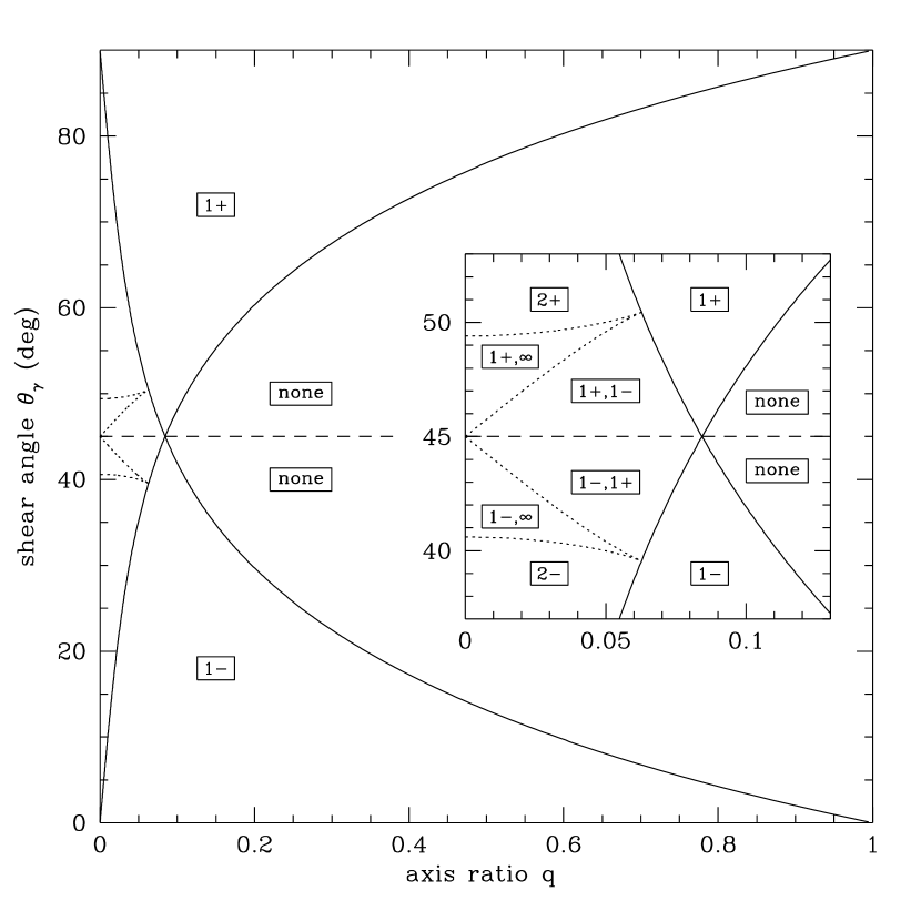
Figure 12: The $(q,\theta_{\gamma})$ plane for galaxy+shear models. The inset shows a closeup of the region with $q$ small and $\theta_{\gamma}\simeq 45^{\circ}$. The solid curves show solutions to eq. (A7), while the dotted curves show solutions to eq. (A8). The solid curves intersect at $\theta_{\gamma}=45^{\circ}$ and $q=\radical"270370{7/(493+90\radical"270370{30})}=0.0843$. The dotted curves meet the solid curves at $q=8-3\radical"270370{7}=0.0627$ and $c_{\gamma}=\pm 1/\radical"270370{28}$ or $\theta_{\gamma}=39.55^{\circ}$ and $50.45^{\circ}$. The curves divide the plane into nine regions. Each region has a distinct set of envelopes containing swallowtail models, as explained in Appendix A.

With these results we can understand the $(q,\theta_{\gamma})$ plane as shown in Figure 12. The curves given by eqs. (A7) and (A8) define nine different regions where the swallowtail envelopes (the parameter regions with $F<0$) have the following properties:

none $$:$$ no envelopes

$$1+ : \gamma>0$$ one envelope, with

$$2+ : \gamma>0$$ two envelopes, both with

$$1+,1- : \gamma>0 \gamma<0$$ two envelopes, one with and one with

$$1+,\infty : \gamma>0 \gamma\to\pm\infty$$ one finite envelope with , and envelopes with

$$1- : \gamma<0$$ one envelope, with

$$2- : \gamma<0$$ two envelopes, both with

$$1-,1+ : \gamma<0 \gamma>0$$ two envelopes, one with and one with

$$1-,\infty : \gamma<0 \gamma\to\pm\infty$$ one finite envelope with , and envelopes with

Negative shear is unphysical (see §2.2), so we are interested only in envelopes with $\gamma>0$, which occur in six of the nine regions: $(1+)$; $(2+)$; $(1+,1-)$; $(1+,\infty)$; $(1-,1+)$; and $(1-,\infty)$.

With this detailed knowledge of the $(q,\theta_{\gamma})$ plane, we can use a numerical root finder with eq. (A2) to obtain the envelope of swallowtail models. The results are shown and discussed in §3.3. In particular, Figures 4–6 show envelopes in the $(q,\gamma)$ plane for different values of $\theta_{\gamma}$. Each envelope corresponds to a particular horizontal line in Figure 11. Each point where this line crosses a curve in the $(q,\theta_{\gamma})$ plane corresponds to a cusp in the envelope in the $(q,\gamma)$ plane.

Appendix B Models that can produce 8 images

We can also ask what range of swallowtail models produce overlapping swallowtails that bound 8-image regions (e.g. Figure 3b). We cannot answer this question analytically for arbitrary values of the shear angle $\theta_{\gamma}$. However, from the examples in §3.2 we expect that overlapping swallowtails occur only when the shear is nearly orthogonal to the galaxy, and the case with $\theta_{\gamma}=90^{\circ}$ can be studied analytically. When $\theta_{\gamma}=90^{\circ}$ the system has reflection symmetry, so the points on the caustic with $\theta=0$ and $\theta=\pi/2$ are always cusps, no matter how convoluted the rest of the curve is. (These cusps are indicated in Figure 3.) Moreover, the $\theta=0$ cusp always opens to the left, and the $\theta=\pi/2$ cusp always opens downward. Label the $\theta=0$ cusp position $(u_{H},0)$ and the $\theta=\pi/2$ cusp position $(0,v_{V})$ (H for horizontal, V for vertical). From Figure 3 we see that there are overlapping swallowtails only if $u_{H}$ and $v_{V}$ are both positive. (If one is positive and one negative then there are swallowtails that do not overlap.) We can use eq. (13) to rewrite the conditions $u_{H}>0$ as follows:

$$u_{H}>0\ \Longleftrightarrow\ \gamma<\gamma_{H}(q) \equiv {1-E_{H}(q)\over 1+E_{H}(q)}\,,$$ (B1)

$$\mbox{where}\quad E_{H}(q) \equiv {q\over\sqrt{1-q^{2}}}\,\tan^{-1}\left({\sqrt{1-q^{2}}\over q}\right)\,.$$

We can similarly rewrite the condition $v_{V}>0$:

$$v_{V}>0\ \Longleftrightarrow\ \gamma>\gamma_{V}(q) \equiv {E_{V}(q)-1\over E_{V}(q)+1}\,,$$ (B2)

$$\mbox{where}\quad E_{V}(q) \equiv {1\over\sqrt{1-q^{2}}}\,\tanh^{-1}\left(\sqrt{1-q^{2}}\right)\,.$$

For any galaxy axis ratio $0\leq q\leq 1$, these functions satisfy $\gamma_{V}(q)\leq\gamma_{H}(q)$. Thus the condition for overlapping swallowtails is $\gamma_{V}(q)<\gamma<\gamma_{H}(q)$, and this result is shown in Figure 4.

Figure 1: Sample caustics and pseudo-caustics for models with a singular isothermal ellipsoid galaxy and an external shear. The smooth elongated curves are the pseudo-caustics and the diamond-shaped curves are the astroid caustics. All panels have a galaxy with a projected axis ratio $q=0.5$ and a shear whose magnitude $\gamma$ and direction $\theta_{\gamma}$ are indicated. The axes are labeled in terms of the natural lensing length scale $b_{\rm SIS}$ from eq. (9).

Figure 2: Examples of “swallowtail” caustics produced when the ellipticity and shear are nearly orthogonal. The left-hand panels show the tangential caustics and sample source positions; the pseudo-caustics are larger than the frames. The right-hand panels show the corresponding tangential critical curves and image positions. All models have $q=0.5$ and $\gamma=0.22$ and the specified shear direction $\theta_{\gamma}$. The points show that a source inside the astroid but outside the swallowtails produces 4 images (case a); a source inside a swallowtail produces 6 images (case b); and a source inside overlapping swallowtails produces 8 images (case c). The total magnification of the sample images in cases a, b, and c is 76.8, 178.3, and 266.2, respectively.

Figure 3: The dependence of swallowtails on the shear. All models have $q=0.5$ and an orthogonal shear ($\theta_{\gamma}=90^{\circ}$) with the specified magnitude $\gamma$. The points indicate the cusps with $\theta=0$ (on the horizontal axis) and $\theta=\pi/2$ (on the vertical axis); see Appendix B for details.

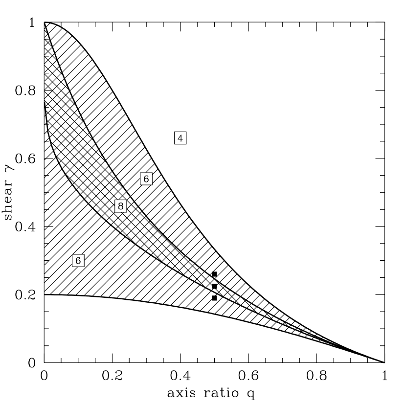
Figure 4: The envelope of galaxy+shear models that can produce at least 6 images in the $(q,\gamma)$ plane, for a shear orthogonal to the lens galaxy ($\theta_{\gamma}=90^{\circ}$). Models in the cross-hatched region have overlapping swallowtails and can produce up to 8 images. Models in the shaded region have non-overlapping swallowtails and can produce up to 6 images. Models outside the shaded region do not have swallowtails and can produce at most 4 images. The curves bounding these regions are given by eqs. (A5), (B1), and (B2) in Appendices A and B. The three filled points indicate the locations of the three sample models shown in Figure 3.

Figure 5: Similar to Figure 4, but for different values of the shear angle near $\theta_{\gamma}\simeq 90^{\circ}$. Only the swallowtail envelope is shown (not the envelope for overlapping swallowtails). The outer envelope corresponds to $\theta_{\gamma}=90^{\circ}$, and moving inward the line type alternates as $\theta_{\gamma}$ decreases by $2^{\circ}$.

Figure 6: Similar to Figure 4, but for values of the shear angle near $\theta_{\gamma}\simeq 45^{\circ}$. Note that the vertical axes are $\log\gamma$ instead of $\gamma$. For $\theta_{\gamma}>50.45^{\circ}$ there are two closed envelopes. For $50.45^{\circ}>\theta_{\gamma}>45^{\circ}$ there is one closed envelope and one envelope that extends to $\gamma\to+\infty$. For $45^{\circ}>\theta_{\gamma}>39.55^{\circ}$ there is only the envelope that extends to infinity. For $\theta_{\gamma}<39.55^{\circ}$ there is no envelope. (Also see Figure 12 in Appendix A.)

Figure 7: The dependence of swallowtails on the galaxy core radius $s$. All models have $q=0.5$ and $\gamma=0.22$. The top panels show models with $\theta_{\gamma}=88^{\circ}$, while the bottom panels show models with $\theta_{\gamma}=90^{\circ}$. For comparison, Figures 2b and 2c show the same models in the limit $s=0$.

Figure 8: The caustics for a galaxy with $q=0.5$ perturbed by an external shear (top panels), and by a singular isothermal sphere at angle $\theta_{\gamma}=90^{\circ}$ and distance $d$ (bottom panels). The strength of the perturbation is given by $\gamma$. Each frame is $0.6\,b_{\rm SIS,1}$ on a side. In some cases with large $\gamma$ and small $d$, the caustics of the main lens galaxy and the perturber merge and become larger than the frames.

Figure 9: Similar to Figure 8, but for $\theta_{\gamma}=88^{\circ}$. Each frame is $0.6\,b_{\rm SIS,1}$ on a side.

Figure 10: Differential cross sections (in units of $b_{\rm SIS}^{2}$) vs. logarithm of magnification $A$ for 2-, 4-, 6-, and 8-image lenses produced by galaxy+shear lens models. The cross-sections are computed for a point source in a square with side-length of $5\,b_{\rm SIS}$. The lens galaxy axis ratio is $q=0.5$, the shear amplitude is $\gamma=0.22$, and the shear direction is indicated; the cases correspond to those shown in Figure 2.

Figure 11: Sample images for a source with finite radius $R_{\rm src}$. The lens model and source position are the same as in Figure 2b. The images are distorted tangentially relative to the lens galaxy, and as the source gets bigger they smear out into an Einstein ring.

References

- (1) Augusto, P., Wilkinson, P. N., Browne, I. W. A. 1996, in Kochanek, C.S. Hewitt, J.N. (eds.), IAU 173, Melbourne, Astrophys. Applications of Gravitational Lensing, Kluwer, 399
- (2) Barkana, R., & Loeb, A. 1999, preprint astro-ph/9906398
- (3) Browne, I. W. A. 2000, in Gravitational Lensing: Recent Progress and Future Goals, ASP conference series, eds. T. G. Brainerd & C. S. Kochanek, in press
- (4) Erdl, H., & Schneider, P. 1993, A&A, 268, 453
- (5) Fabbiano, G. 1989, ARA&A, 27, 87
- (6) Fischer, P., et al. 1999, preprint astro-ph/9912119
- (7) Grogin, N. A., & Narayan, R. 1996, ApJ, 464, 92; erratum, 1996, ApJ, 473, 570
- (8) Gunn, J. E., et al. 1998, AJ, 116, 3040
- (9) Hewitt, J. N., Turner, E. L., Schneider, D. P., Burke, B. F., & Langston, G. I. 1988, Nature, 333, 537
- (10) Hogg, D. W., & Blandford, R. D. 1994, MNRAS, 268, 889
- (11) Jackson, N., Helbig, P., Browne, I., Fassnacht, C. D., Koopmans, L., Marlow, D., & Wilkinson, P. N. 1998, A&A, 334, L33
- (12) Kassiola A., & Kovner, I. 1993, ApJ, 417, 450
- (13) Keeton, C. R., & Kochanek C. S. 1998, ApJ, 495, 157
- (14) Keeton, C. R., Kochanek, C. S., & Seljak, U. 1997, ApJ, 482, 604
- (15) Keeton, C. R., Falco, E. E., Impey, C. D., Kochanek, C. S., Lehár, J., McLeod, B. A., Rix, H.-W., Muñoz, J. A., & Peng, C. Y. 2000a, preprint astro-ph/0001500
- (16) Keeton, C. R., Kochanek, C. S., & McLeod, B. A. 2000b, in preparation
- (17) Kochanek, C. S. 1995, ApJ, 445, 559
- (18) Kochanek, C. S. 1996, ApJ, 473, 595
- (19) Kochanek, C. S., & Apostolakis, J. 1988, MNRAS, 235, 1073
- (20) Koopmans, L. V. E., & Fassnacht, C. D. 1999, ApJ, 527, 513
- (21) Koopmans, L. V. E., et al. 1999, MNRAS, 303, 727
- (22) Kormann, R., Schneider, P., & Bartelmann M. 1994, A&A, 284, 285
- (23) Kundić, T., Cohen, J. G., Blandford, R. D., & Lubin, L. M. 1997a, AJ, 114, 507
- (24) Kundić, T., Hogg, D. W., Blandford, R. D., Cohen, J. G., Lubin, L. M., & Larkin, J. E. 1997b, AJ, 114, 2276
- (25) Lawrence, C. R., Schneider, D. P., Schmidet, M., Bennett, C. L., Hewitt, J. N., Burke, B. F., Turner, E. L., & Gunn, J. E. 1984, Science, 223, 46
- (26) Maoz, D., & Rix, H.-W. 1993, ApJ, 416, 425
- (27) Myers, S. T., et al. 1999, AJ, 117, 2565
- (28) Nair, S., & Garrett, M. A. 1997, MNRAS, 284, 58
- (29) Rix, H.-W., de Zeeuw, P. T., Carollo, C. M., Cretton, N., & van der Marel, R. P. 1997, ApJ, 488, 702
- (30) Rusin, D., Hall, P. B., Nichol, R. C., Marlow, D. R., Richards, A. M. S., & Myers, S. T. 1999, preprint astro-ph/9911420
- (31) Schechter, P. L. 2000, in Gravitational Lensing: Recent Progress and Future Goals, ASP conference series, eds. T. G. Brainerd & C. S. Kochanek, in press (also preprint astro-ph/9909466)
- (32) Schneider, P., Ehlers, J., & Falco, E. E. 1992, Gravitational Lenses (New York: Springer)
- (33) Sykes, C. M., et al. 1998, MNRAS, 301, 310
- (34) Tonry, J. L. 1998, AJ, 115, 1
- (35) Tonry, J. L., & Kochanek, C. S. 1999, AJ, 117, 2034
- (36) Turner, E. L. 1980, ApJ, 242, L135
- (37) Turner, E. L., Ostriker, J. P., & Gott, J. R. 1984, ApJ, 284, 1
- (38) Walker, R. J. 1955, Algebraic Curves (Oxford University Press)
- (39) Wallington, S., & Narayan, R. 1993, ApJ, 403, 517
- (40) Walsh, D., Carswell, R. F., & Weymann, R. J. 1979, Nature, 279, 381
- (41) Weymann, R. J., et al. 1980, Nature, 285, 641
- (42) Witt, H. J. 1996, ApJ, 472, L1
- (43) Witt, H. J., & Mao, S. 1997, MNRAS, 291, 211
- (44) Witt, H. J., & Mao, S. 2000, MNRAS, 311, 689