The spectral variations of the O-type runaway supergiant HD 188209

Abstract

We report spectral time series of the late O-type runaway supergiant HD 188209. Radial velocity variations of photospheric absorption lines with a possible quasi-period $\sim$ 6.4 days have been detected in high-resolution echelle spectra. Night-to-night variations in the position and strength of the central emission reversal of the H${\rm\alpha}$ profile occuring over ill-defined time-scales have been observed. The fundamental parameters of the star have been derived using state-of-the-art plane–parallel and unified non-LTE model atmospheres, these last including the mass-loss rate. The derived helium abundance is moderately enhanced with respect to solar, and the stellar masses are lower than those predicted by the evolutionary models. The binary nature of this star is not suggested either from Hipparcos photometry or from radial velocity curves.

1 Introduction

Runaway O stars have been defined as a group by Blaauw (1961), who introduced the term runaway to describe the space motions of AE Aur and $\mu$ Col. Blaauw (1961) has also suggested that such stars were ejected in the breakup of binary systems in supernova explosions by their companions. In later evolutionary stages, the initial secondary appears as a most massive star and transfers matter to the compact companion (the initial primary) making the system appear as a massive X-ray binary (van den Heuvel 1976). Given the possibility of the binary nature of runaway stars, it appears to be an important task to measure the radial velocity (RV) variations of the photospheric lines. Systematic searches for RV variations have been made in order to assess the binary frequency of O stars (e.g. Garmany, Conti & Massey 1980; Stone 1982, Gies 1987). In many cases the amplitude of RV variations is quite large, and the additional presence of a clear periodicity immediately suggests a binary nature for the system. However, there are stars which show more complicated RV curves, and the interpretation of their spectral variability is not straightforward. HD 188209 (O9.5Iab) is one of those objects. Garmany et al. (1980) have concluded from three spectra that this star is probably not a binary, and that the RV variations must be attributed to atmospheric motions. This conclusion was supported by Musaev & Chentsov (1988). However, based on 21 measurements Stone (1982) has concluded that HD 188209 can be considered as a spectroscopic binary with a period 57 days and small semiamplitude. More recently, Fullerton, Gies & Bolton (1996) included HD 188209 in a large sample of stars investigated on the presence of line profile variability (LPV) and found LPVs only in He i 5876 Å. However, they did not flag HD 188209 as a velocity variable (their Table 10).

The binarity of many O supergiants has been proposed recently by Thaller (1997). The fact that binaries have a higher incidence and an H$\alpha$ emission strength in post-MS stages may indicate that wind interactions are a common source of emission in massive stars. In other words, even in cases where RV measurements are not available, the presence of H${\rm\alpha}$ emission in a spectrum could be linked with colliding winds. One needs to study orbital phase variations in the H${\rm\alpha}$ profile in order to be sure that the latter is due to colliding winds instead of some other mechanism. Note that HD 188209 is an X-ray source detected by ROSAT (Berghoefer, Schmitt & Cassinelli 1996).

In this paper we focus on the high-resolution spectroscopic data of HD 188209. Our observations can possibly account for the small semi-amplitudes and eccentric orbits of this binary candidate since they have been accumulated at different periods over a long baseline.

2 Observations

The observations have been carried out in different runs (Table 1) using the the Coudé Echelle Spectrometer (Musaev 1993) at the 1-m telescope of the Special Astrophysical Observatory of the Russian Academy of Science. Most of the spectra have a signal-to-noise ratio S/N$\geq$100 per resolution element, and an average resolution $R=$ 40000 in the wavelength region 4400–7000 Å. Preliminary reduction of the echelle spectra CCD images was made using the dech code (Galazutdinov 1992), which allows the flat-field division, bias/background subtraction, one-dimensional spectrum extraction from two-dimensional images, excision of cosmic-ray features, spectrum addition, correction for diffuse light, etc. Numerous bias, flat-field have been obtained every night. Each image was subject to a bias-frame subtraction and flat-field division using nightly means. Comparison exposures of a Th-Ar lamp were taken for each stellar spectrum. The control measurements of interstellar Ca ii   and Na i  D lines revealed a small scatter of 0.8 $~{}{\rm km}~{}{\rm s}^{-1}$ (1 $\sigma$). However, the 1 $\sigma$ dispersion of the velocity of the DIB was 1.5 $~{}{\rm km}~{}{\rm s}^{-1}$. These interstellar lines have been used to align all the spectra in the time series accurately. As an indicator of the overall precision of our measurements we have adopted 1 $\sigma$ dispersion 1.5 $~{}{\rm km}~{}{\rm s}^{-1}$ of the velocity of the DIB. All stellar absorption lines exhibited variations about their respective mean velocities at least 2-3 times the dispersion of the DIB velocities. The mean rms obtained from different dispersion curves was at least 0.003 Å. The Coudé Echelle Spectrograph was not a subject to mechanical and/or thermal instabilities.

We used a 580$\times$530 (pixel size 24 $\times$ 18 $\mu$m) CCD camera in all runs except 8 and 9. The last run was carried out using the Coudé Echelle Spectrograph (Musaev, 1999) at the 2-m telescope located in Terskol (North Caucasus, Russia). The CCD used in last two runs had a larger matrix (WI 1242$\times$1152 pixel with pixel size 22.5 $\times$ 22.5 $\mu$m) allowing a coverage in a single exposure of the region $\sim$ 3500–10100 Å  with almost the same resolution.

Table 1: Journal of Observations. The second column gives the universal plus exposure time and in third column is the spectral region. The S/N ratio is given at 6600 Å.

Run	Date	UT + EXP	Region	S/N
	(dd.mm.yy)		(Å)
1	14.06.93	20h 35m+30m	4800–7500	100
	07.07.93	20h 40m+30m	4420–6710	100
	08.07.93	19h 25m+20m	4350–4510	200
			6540–6720
2	04.09.93	21h 53m+30m	4350–4510	200
			6540–6720
	05.09.93	23h 55m+20m	4350–4510	200
			6540–6720
	06.09.93	20h 40m+20m	4350–4510	200
			6540–6720
	07.09.93	20h 07m+45m	4350–4510	200
			6540–6720
	09.09.93	22h 40m+45m	4350–4510	200
			6540–6720
3	07.10.93	17h 46m+60m	4370–6720	150
	08.10.93	17h 35m+60m	4370–6720	150
	09.10.93	17h 40m+60m	4370–6720	150
	10.10.93	18h 32m+60m	4370–6720	150
4	31.10.93	16h 22m+30m	4330–4520	200
			6540–6720
	01.11.93	20h 32m+30m	4330–4520	200
			6540–6720
	02.11.93	16h 18m+45m	4400–6800	100
5	24.11.93	17h 56m+45m	4420–7000	100
	25.11.93	17h 02m+60m	4420–7000	150
	27.11.93	19h 15m+60m	4420–7000	150
	28.11.93	16h 50m+60m	4420–7000	150
	29.11.93	16h 41m+60m	4420–7000	150
	30.11.93	15h 50m+60m	4420–7000	150
	02.12.93	16h 22m+60m	4420–7000	150
	05.12.93	17h 08m+60m	4420–7000	150
6	16.09.94	17h 27m+60m	4420–7000	150
	17.09.94	17h 26m+60m	4420–7000	150
	18.09.94	17h 18m+60m	4420–7000	150
	19.09.94	17h 36m+60m	4420–7000	150
	20.09.94	21h 21m+60m	4420–7000	150
	21.09.94	18h 01m+60m	4420–7000	150
7	13.10.94	17h 00m+60m	4350–6710	150
	15.10.94	16h 40m+60m	4350–6710	150
	16.10.94	20h 20m+60m	4350–6710	150
	17.10.94	18h 01m+60m	4350–6710	150
	25.10.94	18h 00m+60m	4350–6710	150
	27.10.94	19h 06m+40m	4350–6710	100
	29.10.94	16h 36m+40m	4350–6710	100
8	15.05.97	00h 35m+45m	3380–10060	200
	15.05.97	21h 56m+60m	3380–10060	250
	16.05.97	21h 09m+60m	3380–10060	250
	30.08.97	19h 03m+30m	4420–6800	100
9	08.03.98	02h40m+30m	3560–10060	200
	09.03.98	01h50m+45m	3560–10060	250
	10.03.98	02h02m+45m	3560–10060	250
	11.03.98	01h32m+20m	3560–10060	200

Figure 1: Hipparcos photometry of HD 188 209.

3 Photometry

The photometry of HD 188209 obtained with Hipparcos (ESA 1997) is presented in Figure 1. The approximate response curve for the Hp_dc passband (see van Leeuwen et al. 1997) is very extended with a maximum at $\sim$ 4500 Å. Our observations did not reveal a strong variability in the equivalent widths of the strongest lines in the spectrum of HD 188209, which suggests that the variations detected by Hipparcos in the Hp_dc band are due to changes in the continuum flux. The mean value of Hp_dc=5.605 has a standard deviation 0.0155. The level of photometric variability is significant and cannot be ascribed to standard errors in the Hp_dc magnitude of the order of 0.005 (van Leeuwen et al. 1997). Tests on the periodicity of the photometric variations were performed but no convincing period has been found. However, considering the large gaps in different Hipparcos measurements we cannot definitely rule out short-term photometric periodicity.

4 Fundamental Parameters of HD 188209

4.1 Plane–parallel analysis

To analyse the spectrum of HD 188209 we first determine the rotational velocity from the width of 11 metal lines of C, N, O, Si, Mg and Ca, adopting a Gaussian instrumental profile with a FWHM of 0.13 Å. The resulting value was a projected rotational velocity of 82.0 $\pm$ 8.5 km s^-1, in good agreement with the value of 87$~{}{\rm km}~{}{\rm s}^{-1}$ reported by Penny (1996), and between those given by Conti and Ebbets (1977) and Howarth et al. (1997) who give 70 and 92$~{}{\rm km}~{}{\rm s}^{-1}$, respectively.

The method followed in determining the stellar parameters from the spectrum using NLTE, plane–parallel hydrostatic model atmospheres has been described in detail by Herrero et al. (1992, and references therein). Briefly, we determine, at a fixed helium abundance, the gravity that best fits the different H and He profiles at a given temperature for a set of temperatures. If the abundance is right, the lines in the $T_{\rm eff}$–$\log g$  diagram will ideally cross at a point, giving the stellar $T_{\rm eff}$  and $\log g$. Usually, they form an intersection region, whose central point is taken as giving the stellar parameters, and whose limits give the adopted error. If the lines do not cross at any point, the helium abundance is changed. The helium abundance giving the smaller intersection region for all profiles is the one selected. The center of the intersection region is taken again as that giving the stellar parameters.

Recently, McErlean, Lennon & Dufton [1998] and Smith & Howarth  [1998] have shown that different He i  lines give different helium abundances in the region of the $T_{\rm eff}$– $\log g$  diagram occupied by HD 188209. They attribute this to the effect of microturbulence and show that a value of around 10 km s^-1 is appropriate for bringing most of the He i  lines into agreement. Thus, we adopt this value for HD 188209 and carry out the analysis in the way described above.

Figure 2: The fit to the HD 188209 lines using unified models. a) H${\rm\gamma}$; b) He i  4471; c) He i  4387; d) He i  4922; e) He ii  4200, and f) He ii  4541 Å(see text for details).

Figure 3: The fit to the HD 188209 lines using unified models. a) H${\rm\gamma}$; b) He i  4471; c) He i  4387; d) He i  4922; e) He ii  4200, and f) He ii  4541 Å(see text for details).

With this method we have determined the stellar parameters of HD 188209. We obtained $T_{\rm eff}$= 31 500 K $\pm^{1000}_{500}$, $\log g$= 3.0 $\pm 0.1$ (uncorrected for centrifugal force; because of the low rotational velocity we neglect this small correction here) and $\epsilon$= 0.12 $\pm 0.03$ (the abundance of helium with respect to the total abundance of hydrogen plus helium, by number; the solar abundance is $\epsilon$= 0.09). The final fits for the H and He lines are shown in Figure 2.

The larger errors towards higher temperatures is due to a small difference in the two spectrograms available for He ii 4541 Å. Using the second one, we would have obtained a $T_{\rm eff}$  of 32 000 K, all other parameters remaining the same. For this reason, we have enlarged the error bar in this direction. Remember that the errors given are formal errors, in the sense that they express the uncertainty in the fit using the models described above.

As has been show by Herrero [1994] the metal opacity in the UV (line blocking) could also affect the value of the parameters determined. However, at the relatively low temperature of HD 188209 the effect would be minor, moving $T_{\rm eff}$  towards higher temperatures within the error box.

With the stellar parameters given above we can determine the radius, luminosity and mass of HD 188209 as described in Herrero et al. (1992). For $M_{\rm v}$= $-$6.0 mag ($M_{\rm bol}$ = $-$9.0 mag) given by Howarth & Prinja (1989) we obtain $R/R_{\odot}$= 20.9, $\log(L/L_{\odot})$= 5.59 and $M/M_{\odot}$= 16.6. The errors are again as in Herrero et al. (1992): $\pm$0.06 in $\log(R/R_{\odot})$, $\pm$0.16 in $\log(L/L_{\odot})$  and $\pm$0.22 in $\log(M/M_{\odot})$.

HD 188209 does not formally show the helium discrepancy, as the solar helium abundance is within the error bars. However, it shows the mass discrepancy: the mass derived from the plane–parallel spectroscopic analysis is, even including the error bars, much lower than the one derived from the evolutionary tracks from Schaller et al. [1992].

4.2 Unified model analysis

After having the parameters from the plane–parallel analysis, we can try to use a spherical, non-hydrostatic model atmosphere in order to improve the already derived parameters and also to obtain the mass-loss rate. In a supergiant like HD 188209 this can have an important impact on the final parameters. Usually, it is also assumed that this will contribute to the reduction in the mass discrepancy.

The unified code we use is that recently developed by Santolaya–Rey, Puls & Herrero [1997]. The reader will find all the details therein, but for our present purposes we mention that the code uses spherical geometry, with a $\beta$–velocity field, and treats the wind and the photosphere in a unified way. It also makes use of the NLTE-Hopf functions. Stark broadening is included in the formal solution, and the model atoms are the same as in the plane–parallel case (slightly adapted for the new program).

We begin by estimating the mass-loss rate from the H${\rm\alpha}$ profile, and then, with this mass-loss rate, we try again to find the best gravity (from the H${\rm\gamma}$ wings), effective temperature and He abundance (from the He ionization equilibrium). With the new parameters, we again try to fit the H${\rm\alpha}$  by varying the mass-loss rate, and so on. In the whole process we take the wind terminal velocity from Haser (1995), who gives 1700 km s^-1. Note that Howarth et al. (1997), give a similar value of 1650 km s^-1.

We have used for the analysis the same lines as in Fig. 2, but have included He i 4471 Å instead of H${\rm\beta}$(that improved as does H${\rm\gamma}$) to show the dilution effect (see below). In Fig. 3 we show the fit of the H${\rm\gamma}$, He i and He ii lines. The adopted parameters are now $T_{\rm eff}$= 31 500 K, $\log g$= 3.00 and $\epsilon$= 0.12, i.e. the same parameters as in the plane–parallel case, even for the gravity (again adopting a microturbulent velocity of 10 km s^-1). Thus, the unified models do not contribute in this case to changes in the mass discrepancy found with the plane–parallel models (nor in the He abundance). We can also see in Fig. 3 that the He i 4471 line shows the well known dilution effect mentioned by Voels et al. [1989], although the other He lines fit perfectly well. This effect merits an explanation.

The fitting of the H${\rm\alpha}$ profile needed to derive the mass-loss rate cannot be done properly. The profile is highly variable, and we have adopted a qualitative approach: we have simply tried to give upper and lower limits to the mass-loss rate. As an example, we illustrate the procedure in Fig. 4, where we show one of the profiles with various mass-loss rates for the stellar parameters given above. The theoretical mass-loss rate values shown in Fig. 4 are log Ṁ= $-$5.70, $-$5.80 and $-$5.90 (with Ṁ in $M_{\odot}$/yr). This situation is similar to that found by Herrero et al. [1995] for Cygnus X–1. The profile shown cannot be adopted as either an average or a representative one, as the profile varies a lot. The figure is only for illustrative purposes. An average logarithmic mass-loss rate for HD 188209 would be between $-$6.0 and $-$5.7. These values are also in agreement with the profiles in Fig. 3, where the adopted mass-loss rate was log Ṁ=$-$5.80 (corresponding to 1.58 10^-6 $M_{\odot}$/yr). We should point out that other values of the mass-loss rate give worse fits to the H${\rm\gamma}$ and He i lines, by strongly modifying the line cores.

5 Radial velocity variations of the absorption lines

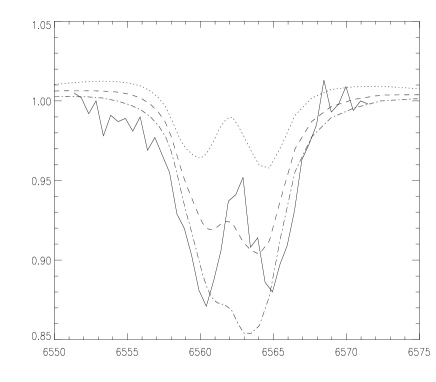
Figure 4: The H${\rm\alpha}$ profiles of HD 188209 observed on 1993 September 7 enclosed by different theoretical profiles calculated for log Ṁ= $-$5.70, $-$5.80 and $-$5.90 (dotted, dashed and dash–dotted lines, respectively) for the parameters given in text. The selected observed H${\rm\alpha}$ profile is neither an average nor representative, and the figure merely illustrates the approach we have followed.

Figure 5: Mean radial velocities of different groups of lines versus TEE. A linear fit (0.1527,-17.05) provides a non-parametric correlation coefficient 0.73.

Figure 6: Standard deviations of mean radial velocities of different groups of lines versus TEE. A linear fit ($-$0.049,8.474) provides a non-parametric correlation coefficient 0.76.

The radial velocity variations in stars can have instrumental, internal (atmospheric) and/or external (Keplerian) origin. Instrumental effects in our measurements are minimized due to the high resolution and high S/N of the data presented. The internal accuracy achieved for the wavelength calibrations is of the order 1.5 ${\rm km}~{}{\rm s}^{-1}$ as derived from the scatter of measured radial velocities of interstellar and telluric lines in the spectra. Note that all former studies of HD 188209 (except for five spectra obtained by Fullerton et al. 1996) were based on the photographic spectra. Atmospheric pulsations of early-type stars have been the subject of extensive studies (e.g. Burki 1978; Bohannan & Garmany 1978, Kaufer et al. 1997, Fullerton et al. 1996) and have been reviewed by Baade (1988, 1998). Gies (1987) has compared the velocity distribution and binary frequency among 195 Galactic O-type stars (cluster and association, field and runaway) and found a deficiency of spectroscopic binaries among field stars (and especially among the runaway). The most comprehensive radial velocity studies of OB and BA supergiants to date are those of Fullerton et al. (1996) and Kaufer et al. (1996; 1997). Radial pulsation periods with P$\leq$5^d have been predicted for O-type supergiants (Burki 1978; de Jager 1980; Levy et al. 1984). The presence of pulsations or random motions in stellar atmospheres results in complex velocity curves for different spectral lines due to stratification effects (Abt 1957). This is in contrast to Keplerian motions where all the lines vary synchronously with time (Ebbets 1979; Garmany et al. 1980). However, in many cases the amplitude of the RV variations does not exceed 25–30 ${\rm km}~{}{\rm s}^{-1}$, and it is very difficult to distinguish whether these variations are of an internal or an external nature. Additional difficulty comes from the possible presence of non-radial pulsations (NRP). Variable profiles (LPVs) have been detected in many narrow-line supergiants (e.g. Baade 1988; Kaufer et al. 1997; Fullerton et al. 1996) and in some cases they correspond to the radial velocity variations measured in photographic spectra. However, in contrast to broad-line supergiants, clear evidence of NRPs in narrow- and intermediate-line O-type supergiants has not yet been found. Although LPVs are a common occurrence among the O-type stars, some of them (like HD 34656; Fullerton, Gies & Bolton 1991) show a variability which consists of cyclical fluctuations in radial velocity due to pulsations in a fundamental mode.

Figure 7: Lomb-Scargle (top panel) and CLEAN periodograms of the average RV for each date obtained by averaging the RVs of all the groups.

Figure 8: The fitting of a sin curve to folded data for a period 6.4 days. The curve is derived for RV=$-$9.8+4.17$\sin$ [2$\pi$(JD-318.629)/6.406].

Careful inspection of our time series showed that all absorption lines varied in position over the course of a day. We have detected a few asymmetric profiles of He lines but there were no signatures of moving features. It is however possible that the S/N ratio of our data is not high enough to trace LPVs. Small distortions in profile shape are typically less than 1% of the continuum strength and a minimum S/N ratio required would be at least 300 (Fullerton et al. 1996).

5.1 The velocity-excitation relationship

We have selected unblended lines by utilizing theoretical synthetic spectra computed for the model atmosphere of HD 188209 and measured RVs by fitting a Gaussian to the line profile. The following groups of lines have been selected: He i (4921, 4471, 4713, 5015, 5047, 5876, 6678 Å), He ii (5411, 4541, 4686 Å), Si iv (4654, 4631 Å), C iii (4650, 4647, 5696 Å), Si iii (4567, 4552, 4574 Å), C iv (5801, 5811 Å), N iii (4514, 4510, 4518, 4523 Å), O ii 4661 Å and Mg ii  4481 Å. The average RVs computed for each of these groups of lines are listed in Table 2. It is normally assumed that lines of different total excitation energy (TEE, ionization energy plus excitation energy of the lower level) form in different layers of the atmosphere (Hutchings 1976). However, it is not clear whether the stratification exists in a dynamically active, pulsating atmosphere. One can assume that the time scale of dynamical processes (pulsations, stochastic motions etc.) is much less than the time necessary for the establishment of radiative equilibrium. Thus, while pulsating, the atmosphere is supposed to pass through a chain of hydrostatic stages. The assumption that TEE correlates with line formation depths can be tested as well. We applied our plane–parallel models to compute formation depths of the line cores of the He i and He ii lines. It appeared that the core of the strong He ii 4686 Å line forms much closer to the surface (at column mass $\sim$ 0.01 g cm^-2) than any of the He i lines. However, this was not the case with the two other He ii lines (5411 and 4541 Å) we used in our study. Similar tests have been carried out for other groups of lines but assuming an LTE line formation. These exercises suggest that before combining lines in different groups and computing their average RVs, one has to be sure (of course under the assumption that our plane–parallel models are applicable) that their depths of formation are similar.

Table 2: Radial velocities of different groups of lines.

Date	He i	He ii	Si iv	C iii	Si iii	C iv	N iii	O ii 4661 Å	Mg ii 4481 Å
TEE (eV)	21	75	57	54	35	85	57	36	8.5
2449176.36	$-$12.3	$-$11.2	$-$6.3	$-$8.1	$-$15.9	$-$13.2	$-$8.4	$-$26.4	$-$19.4
2449268.24	$-$5.9	$-$1.4	6.9	$-$4.9	$-$13.8	$-$2.9	$-$5.6	$-$18.8	$-$1.3
2449269.23	$-$10.9	$-$2.1	$-$0.3	$-$11.7	$-$15.1	$-$4.8	$-$8.0	$-$24.1	$-$15.3
2449270.24	$-$10.3	$-$8.1	5.5	$-$7.5	$-$11.7	$-$0.1	$-$6.8	$-$12.8	$-$11.6
2449271.27	$-$15.7	$-$16.5	$-$7.6	$-$17.4	$-$35.5	$-$16.9	$-$12.3	$-$18.2	$-$14.9
2449294.18	7.9	11.1	6.4	$-$0.7	$-$4.6	$-$1.5	2.4	$-$4.4	$-$0.6
2449316.25	$-$17.3	$-$6.5	$-$1.6	$-$13.7	$-$25.3	$-$0.7	$-$10.8	$-$22.7	$-$4.3
2449317.21	$-$17.2	$-$12.9	$-$13.5	$-$10.4	$-$22.5	$-$14.7	$-$12.2	$-$24.9	$-$20.9
2449319.30	$-$4.5	$-$1.6	3.3	3.1	$-$17.1	$-$6.1	$-$5.6	$-$15.7	$-$5.4
2449320.20	$-$8.5	2.4	1.5	$-$1.4	$-$23.0	$-$6.0	$-$1.3	$-$27.6	$-$12.2
2449321.20	$-$2.6	2.7	8.4	1.2	$-$3.9	$-$0.2	0.1	$-$14.9	$-$6.5
2449322.16	$-$16.0	$-$7.5	$-$3.5	$-$9.1	$-$16.3	$-$11.9	$-$11.5	$-$28.5	$-$38.1
2449324.18	$-$14.8	$-$5.2	$-$7.1	$-$9.9	$-$20.9	$-$5.8	$-$10.6	$-$33.5	$-$36.2
2449327.21	$-$1.3	$-$1.6	8.6	$-$3.7	1.4	1.6	$-$3.7	$-$20.5	$-$35.8
2449612.23	$-$15.3	$-$11.1	$-$13.9	$-$11.7	$-$22.7	$-$11.5	$-$11.9	$-$17.2	$-$18.8
2449613.23	$-$10.6	$-$6.2	$-$7.9	$-$8.6	$-$12.7	$-$5.6	$-$6.2	$-$15.8	$-$11.0
2449614.22	$-$14.5	$-$8.7	$-$8.2	$-$10.4	$-$19.6	$-$6.6	$-$8.5	$-$16.9	$-$9.6
2449615.23	$-$9.2	$-$4.7	$-$1.6	$-$12.3	$-$16.7	$-$4.9	$-$6.4	$-$15.7	$-$22.9
2449616.39	$-$10.2	$-$6.4	$-$5.4	$-$8.7	$-$16.2	$-$4.6	$-$5.2	$-$14.2	$-$20.0
2449617.25	$-$15.6	$-$7.6	$-$9.4	$-$11.5	$-$23.8	$-$10.4	$-$10.7	$-$23.2	$-$18.2
2449639.21	$-$0.5	0.3	2.3	$-$0.4	$-$8.7	$-$1.4	0.2	$-$13.9	$-$6.5
2449641.19	$-$2.0	3.7	$-$1.1	$-$4.1	$-$6.3	$-$4.1	$-$3.4	$-$10.1	$-$9.5
2449642.35	$-$9.7	$-$3.1	$-$3.1	$-$5.9	$-$17.2	$-$7.1	$-$5.9	$-$16.3	$-$14.9
2449643.25	$-$6.1	$-$2.7	$-$1.2	$-$6.9	$-$14.9	$-$1.6	$-$5.0	$-$6.4	$-$18.0
2449651.25	$-$13.4	$-$13.3	$-$8.3	$-$12.3	$-$19.9	$-$10.5	$-$11.8	$-$23.1	$-$18.3
2449653.30	$-$6.4	$-$0.2	$-$5.5	$-$6.4	$-$9.9	$-$8.5	$-$7.2	$-$25.0	$-$11.5
2449655.19	$-$8.2	$-$4.3	$-$3.6	$-$7.5	$-$3.4	$-$3.3	$-$7.8	$-$15.7	$-$9.7
2450583.52	$-$11.6	$-$7.5	$-$7.0	$-$16.0	$-$15.6	$-$9.1	$-$11.3	$-$16.4	$-$13.9
2450584.41	$-$13.4	$-$5.8	$-$10.8	$-$11.6	$-$15.9	$-$5.6	$-$11.4	$-$19.9	$-$15.3
2450585.38	$-$19.2	$-$16.9	$-$13.9	$-$14.6	$-$24.9	$-$8.9	$-$14.2	$-$25.3	$-$31.4
2450691.25	$-$7.6	$-$8.6	$-$3.2	5.6	$-$8.9	$-$7.1	$-$4.8	1.6	$-$5.9
2450880.61	$-$6.5	$-$4.6	$-$3.5	$-$7.8	$-$11.1	$-$5.4	$-$7.8	$-$8.8	$-$17.9
2450881.58	$-$14.4	$-$9.6	$-$7.3	$-$13.1	$-$14.2	$-$6.2	$-$12.1	$-$17.3	$-$23.0
2450882.58	$-$11.0	$-$4.3	$-$4.2	$-$7.7	$-$13.6	$-$1.2	$-$7.3	$-$17.0	$-$13.3
2450883.56	$-$9.1	$-$5.2	$-$4.8	$-$4.6	$-$12.9	$-$2.9	$-$2.7	$-$15.3	$-$11.4
Mean	$-$9.6	$-$5.1	$-$3.4	$-$7.7	$-$15.2	$-$6.0	$-$7.3	$-$17.8	$-$15.5
Stdv	5.8	5.7	6.1	5.3	7.3	4.4	4.1	7.2	9.3

Figure 9: The variety of H${\rm\alpha}$ profiles observed in different runs. A vertical dashed line indicates zero velocity.

The velocity–excitation relationship found for many hot supergiants (Hutchings 1976) exists also in HD 188209. In Figs. 5 and 6 we present plots of mean RV versus TEE and standard deviations of the mean RV versus TEE for the different groups of lines computed for all dates (the last two lines in Table 2). These plots exclude a pure Keplerian motion as the only cause of the RV variations. Pulsations and stochastic motions (intrinsic wind variations caused by some hydrodynamical instabilities) in the wind can bring to the RV variations as well. If we suppose that stochastic variations are not important, then the existence of a standard deviation-TEE relationship would suggest that deeper layers in the atmosphere pulsate with smaller amplitudes. The amplitude of pulsations increases when approaching to the surface.

5.2 The periodicity of the radial velocity variations

The period search was carried out with help of the period package (Dhillon & Privett 1997) of the starlink software. The following strategy was applied when looking for a periodic signal in the RV curves of different groups of lines. Due to the large gaps (especially between runs 5 and 6) in our observations, we first decided to study each of the runs 5, 6 and 7 separately. The clean algorithm (Roberts et al. 1987) was employed to cover a space of loop gains from 0.2 to 0.6 and the number of iterations from 10 to few hundreds. The convergence of the periodograms was achieved for the majority of groups of lines in all three runs. The mean frequency suggested by most of the groups in all three runs is 0.44$\pm$0.05 days^-1 (2.24 days). However, this period is very close to the Nyquist frequency (1/(2$\times$Smallest Data Interval)) of the data and might be misleading.

We have also looked for periodic signals in the combined data of all groups obtained in all runs (Table 2). The maximum and minimum frequencies were set to 100 and 0, respectively. A clean analysis of the time series of the majority of groups revealed a frequency of 0.51$\pm$0.1 days^-1 (1.95 days). The gain factor was 0.1 at the first iteration, then was decreased by 15-20 iteration until stabilization. The average RV for each date obtained by averaging the RVs of all the groups revealed a frequency of 0.47$\pm$0.12 days^-1 (2.1 days). Again, both frequencies are very close to the Nyquist frequency and we should discard them. We must point out that our periodograms did not show any peaks at frequencies smaller than 0.4 days^-1. The next strongest peak which appeared in our periodograms was near 0.156$\pm$0.15 days^-1 (6.4 days). Clearly this period is not affected by sampling. We have also analysed the RV data using the Lomb-Scargle method (Lomb 1976, Scargle 1982) which allows to compute statistical probability of peaks in periodograms. To ensure reliable significance values, the minimum number of permutations was set 100. The probability that the period is not equal to 6.4 days was always less than 30 $\%$. The peak at 6.4 days appears in all periodograms but given its significance value, we cannot definitely rule out its non-physical nature. In Figs. 7 and 8 we show the clean and the lomb-scargle periodograms and the fitting of a sin curve to folded data, respectively.

Figure 10: The radial velocities of blue and red absorption components versus residual intensity of the central emission.

6 Variability of H$\alpha$

All hot supergiants have variable H${\rm\alpha}$ profiles in their spectra (Rosendahl 1973). The shape of the H${\rm\alpha}$ may vary from P Cyg to inverse P Cyg, double-peaked, pure absorption and/or emission (Ebbets 1982) with typical time-scales of the order of days. The nature of this variability is not yet understood. The existence of variable asymmetric outflows/infalls of matter and some corotating structures related to surface inhomogenities and possible magnetic fields have been proposed for BA-type (Kaufer et al. 1996) and O-type (Fullerton et al. 1996; Kaper et al. 1997) supergiants. In addition, there have been detailed studies of the rotating giant loop in $\beta$ Orionis (Israelian, Chentsov & Musaev 1997) and the corotating spiral structures in HD 64760 and HD 93521 (Howarth et al. 1998; Fullerton et al. 1997). It is of course very difficult to distinguish binary systems from single stars without understanding the nature of H${\rm\alpha}$ variability. As Thaller (1997) suggests, the H${\rm\alpha}$ can suffer some peculiar variability due to the colliding winds in a binary system.

The time evolution of H${\rm\alpha}$ profiles in three different runs is shown in Figure 9. The average H${\rm\alpha}$ profile consists of three components, a central emission accompanied by blue and red absorptions. We have not observed a single H${\rm\alpha}$ profile without a central reversal. The emission is not always centered exactly on the rest wavelength but is varying. It may approach the continuum level, go above it and decrease rapidly in strength. Apparently the time-scale of the H${\rm\alpha}$ variability is at least one day. The 5^th run has been divided into two parts (runs 5a & 5b) with four successive nights in each. The H${\rm\alpha}$ variability is observed over a wide range from about $-$400 to 200 ${\rm km}~{}{\rm s}^{-1}$.

We have already seen in Section 4.2 that our spherical unified models can account for the central reversal (or at least set upper and lower limits of the mass-loss). Thus, we know that the central emission forms in the expanding envelope and accounts for the filling-in effect observed in H${\rm\alpha}$, H${\rm\beta}$ and some other lines. The filling-in effect observed in H${\rm\beta}$  correlated perfectly with the strength of the H${\rm\alpha}$ central reversal. The H${\rm\alpha}$  wings originate deep in the atmosphere, whereas the central reversal comes from the thin layers of the envelope. One cannot use the term “underlying photospheric absorption line” since the central reversal is not emitted by a detached layer far from the photosphere. It is important to stress that we deal with a $single$ line formed in a $unified$ model atmosphere. A variable amount of incipient emission can be due to density (or radius) variations in the outer atmosphere. However, these variations are not expected to produce an asymmetry as long as we deal with spherically symmetric mass-loss. Our observations indicate that the velocity of the central emission varies as well. We $do$ expect RV variations in the central emission (the upper atmosphere) since we know that the RVs of all absorption lines vary. The amplitude of the RV variations of Mg ii  4481 Å can reach 30$~{}{\rm km}~{}{\rm s}^{-1}$ (Table 2) and 40$~{}{\rm km}~{}{\rm s}^{-1}$ in H${\rm\beta}$. Thus, it is not unusual for the amplitude of RV variations of the H${\rm\alpha}$ central emission to reach 50$~{}{\rm km}~{}{\rm s}^{-1}$. A period analysis of the RV curves of the central emission resulted in the detection of quasi-periodic variability with a frequency 0.42$\pm$0.14 d^-1 (2.35 days). It turns out that the RV curves of all groups of lines vary in phase. However, the RV curve of the H${\rm\alpha}$ was shifted half phase relative to all groups.

We have measured the RVs of the blue and red absorption components of the H${\rm\alpha}$ and plotted them against the residual intensity of the central emission reversal. This plot (Fig. 10) shows a correlation with a large scatter due to the RV variations of the central reversal. This kind of correlation can be expected when the central reversal is moving up and down relative to a local continuum. We found similar correlations between the RV of the central emission and the residual intensities of the red and blue absorptions. Apparently all the changes observed in the H${\rm\alpha}$ wings at velocities $v\leq-$ 100$~{}{\rm km}~{}{\rm s}^{-1}$ and $v\geq$ +100$~{}{\rm km}~{}{\rm s}^{-1}$ are due to the variations of the central reversal. We do not anticipate such large RV variations deep in the atmosphere where these wings are formed. The conclusion is that the overall shape of the H${\rm\alpha}$ is determined by the central emission.

We have performed a period search of the integrated equivalent width (EW) of the H${\rm\alpha}$ data set and found a maximum in power at frequency 0.22 day^-1. Figures 11 and 12 show the phase diagram for the period 4.41 days and a grey-scale representation of the phase spectrum, respectively. A phase spectrum represents a two-dimensional case of the clean algorithm where each velocity bin of the H${\rm\alpha}$ is treated as a time series of the H${\rm\alpha}$ intensity.

Figure 11: The phase diagram of the EWs of H${\rm\alpha}$.

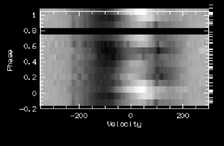
Figure 12: Dynamical phase spectrum of H${\rm\alpha}$.

7 Discussion

Our target belongs to the group of stars for which the existence of a compact companion has been proposed in the literature. The task of disproving or confirming the binary nature of the system can be tackled only if sufficiently accurate analysed observational data are available. In this paper we used state-of-the-art models of atmospheres to determine the fundamental parameters of HD 188209.

To establish the presence of a possible companion we have studied the RVs of absorption lines by combining them in different groups. Fourier analysis based on the iterative clean algorithm was used to search for periodic variability. Unfortunately the time coverage of runs 1–4 and 8–9 was too sparse to set constraints on their time-dependent behaviour. For this reason we first analysed a few runs separately and then utilized the clean algorithm to search for periods in a whole data set. The highest peak in the Fourier power spectrum was centered near the frequency 0.156 day^-1 (6.4 days).

The 6.4 days period can be due to the binary nature of the system if one assumes very small and unlikely values for the mass ratio (q$\leq$0.1). Taking the values derived in this article ($M/M_{\odot}$= 16.6, $R/R_{\odot}$=20.9) and assuming q=0.1, we obtain for the Roche radius and for the major semi-axis of the binary orbit 15 $R_{\odot}$ and 25 $R_{\odot}$, respectively. This simple estimate shows that an O supergiant can hardly fit within the orbit because its Roche radius would be less than the stellar radius. Even if it would fit, the tides in such a tight binary would be very strong making the star to speed up quickly until the rotation period matches the orbit. Even if we assume that the system is very young, it’s hard to explain that the putative orbital period is 2 times shorter than the rotational period (13 days). The second difficulty with the binary interpretation comes from the variability of H$\alpha$. A TVS (temporal variance spectrum, showing the extent and distribution of statistically significant profile variability) has been computed recently (Baade 1998b, Kaper et al. 1998) for 15 spectroscopic binaries and it was found that all they show a characteristic double-peaked profile. This is due to two H$\alpha$ absorption/emission profiles moving in a composite spectra. In our case the H$\alpha$ profile is splitted because of the central emission coming from the lower wind. The last argument comes from the clear relations between excitation energies and radial velocity amplitude and excitation energy and mean radial velocities and from the model atmosphere atmosphere calculations. The latter is a good discriminant between internal variations (pulsations & wind instabilities) and Keplerian motions. In a binary system one would expect all lines to have the same amplitude independent on their TEE.

It has been known for a long time (Abt 1957) that the quasi-periodicity in hot supergiants might be ascribed to radial pulsations. A simple relation (Burki 1978; de Jager 1980) can be used to estimate the period of radial pulsation,

$$\log P_{\rm fund}=10.93-0.5\log(M/M_{\odot})-0.38M_{\rm bol}-3\log T_{\rm eff}$$ (1)

Using the values of parameters obtained in Section 4 we arrive at $P_{\rm fund}$=1.75 d. Note that the form of the relation (1) depends on the stellar evolutionary models and the input parameters; both are subject to large errors. In particular, note that we found no large differences in the parameters determined with plane–parallel and unified model atmospheres. Nevertheless, Levy et al. (1984) have pointed out that periods a factor of 1.5 longer than the corresponding periods of the radial pulsations can be ascribed to non-radial pulsations. This means that a factor of two difference between the evolutionary and the spectroscopic masses can easily result in the mis-identification of the pulsating mode. Another difficulty has been pointed by the referee of the article. A more sophisticated approach shows (Unno et al. 1979) that f-mode pulsation (which is the lowest-frequency mode supported by radial pulsation) periods are about 10 times larger than the one suggested by a period-luminosity relation. In any case, the theoretical period of 1.75 days is very close to the Nyquist frequency of our data which means that we have a little chance to identify it in our data set even if it exists.

Our data not allow to distinguish between pulsations and stochastic variations of the stellar wind. It is also quite possible that we have a combination of both effects.

Note that the projected rotational period of this star ($\sim$ 13 d) is much longer than any of the quasi-periods found in this paper (but of course our runs do not cover a whole rotation cycle). The surface features (if any) will always be visible on the projected disc of the star independently of the inclination angle. Thus, any periods due to the rotation of these features must correspond directly to the rotation period. We do not find any peaks in the power spectra at $\sim$13 d and this leads us to discard rotational modulation as a possible explanation of the RV variations reported here.

The quality and the sampling of our data do not allow a careful study of the line asymmetries, moving components (if later exists) and/or long-term spectroscopic variability to be made. It is quite possible that the non-sinusoidal character of the RV curve for 6.4 days period (Fig 8) is caused by some disturbances due to the NRPs and/or moving features in the profiles plus any stochastic instabilities of the wind. New monitoring with much higher S/N may allow NRPs, multimode pulsations and clearly separate a sinusoidal curve of the radial pulsations to be revealed. However, we found convincing evidence that the atmospheric motions cannot be ascribed solely to Keplerian motions and probably are not of a binary origin.

References

- [1957] Abt, H. A. 1957, ApJ, 126, 138
- [1988] Baade, D. 1988, in O Stars and Wolf-Rayet Stars, eds. Conti, P. and Underhill, A., SP-NASA, Washington DC, p.199
- [1998b] Baade, D. 1998a, in Cyclical Variability in Stellar Winds, eds. Kaper, L. and Fullerton, A., ESO Astrophysics Symposia, Springer, p. 196
- [1998b] Baade, D. 1998b, private communication
- [1996] Berghoefer, T., Schmitt, T., Cassinelli, J. 1996, A&AS, 118, 481
- [1961] Blaauw, A. 1961, Bull. Astr. Inst. Nether., 15, 265
- [1978] Bohannan, B., and Garmany, C. D. 1978, ApJ, 223. 908
- [1978] Burki, G. 1978, A&A, 65, 357
- [1977] Conti, P. & Ebbets, D. 1977, ApJ, 213, 438
- [1997] Dhillon, V. S. & Privett, G. J. 1997, PERIOD, A Time-Series Analaysis Package, Stralink Project, Rutherford Appleton Laboratory
- [1979] Ebbets, D. 1979, ApJ, 227, 510
- [1982] Ebbets, D. 1982, ApJS, 48, 399
- [1997] ESA 1997, The Hipparcos Catalogue, ESA SP-1200
- [1991] Fullerton, A. W., Gies, D. R., Bolton, C. T. 1991, ApJ, 368, L35
- [1996] Fullerton, A. W., Gies, D. R., Bolton, C. T. 1996, ApJS, 103, 475
- [1997] Fullerton, A. W., Massa, D. L., Prinja, R. K., Owocki, S. P., Cranmer, S. R. 1997, A&A, 327, 699
- [1992] Galazutdinov H. A. 1992, Preprint of the Special Astrophysical Observatory of Russian Academy of Science No. 92
- [1980] Garmany, C., D., Conti, P. S., Massey, P. 1980, ApJ, 242, 1063
- [1987] Gies, D. R. 1987, ApJS, 64, 545
- [1995] Haser, S. M. 1995, PhD thesis, Ludwig-Maximillians- Universität München
- [1994] Herrero, A., 1994, Sp. Sc. Rev. 66, 137
- [1995] Herrero A., Kudritzki R. P., Gabler, R., et al., 1995, A&A 297, 556
- [1992] Herrero A., Kudritzki R. P., Vilchez J. M., et al., 1992, A&A 261, 209
- [1985] van den Heuvel, E. P. J. 1976, in Eggleton, P. ed., IAU Symp. 73, Structure and Evolution of Close Binary Systems, Dordrecht, Reidel, p. 263
- [1989] Howarth, I. D., Prinja, R. K. 1989, ApJS, 69, 527
- [1997] Howarth, I. D., Siebert, K. W., Hussain, G. A. J., and Prinja, R. K. 1997, MNRAS, 284, 265
- [1998] Howarth, I. D., Townsend, R. H. D., Clayton, M. J., Fullerton, A. W., Gies, D. R., Massa, D., Prinja, R. K., Reid, A. H. N. 1998, MNRAS, 296, 949
- [1976] Hutchings, J. B. 1976, ApJ, 203, 438
- [1997] Israelian, G., Chentsov, E. and Musaev, F. 1997, MNRAS, 290, 521
- [1980] de Jager C. 1980 The Brightest Stars, Kluwer Dordrecht
- [1997] Kaper, L. et al. 1997, A&A, 327, 281
- [1998] Kaper, L. et al. 1998, in Cyclical Variability in Stellar Winds, eds. Kaper, L. and Fullerton, A., ESO Astrophysics Symposia, Springer, p. 103
- [1997] Kaufer A., Stahl O., Wolf B., Fullerton A., Gäng T., Gummersbach C. A., Jankovics I., Kovács J., Mandel H., Peitz J., Rivinius Th., Szeifert Th. 1997, A&A, 320, 273
- [1996] Kaufer A., Stahl O., Wolf B., Gäng T., Gummersbach C. A., Kovács J., Mandel H., Szeifert, Th. 1996, A&A, 305, 887
- [1997] van Leeuwen, F. et al. 1997, A&A, 323, L61
- [1984] Levy, D., Maeder, A., Noëls, and Gabriel, M. 1984, A&A, 133, 307
- [1976] Lomb, N. R. 1976, Ap. & Sp. Sc., 39, 447
- [1998] McErlean, N., Lennon, D.J., Dufton, P., 1998, A&A, 329, 613
- [1993] Musaev F. 1993, Pis’ma v AZh, 19, 776
- [1993] Musaev F. 1999, Pis’ma v AZh, in press
- [1988] Musaev F., and Chentsov, E. L. 1988, Soviet. Astron. Letters, 14, 226
- [1996] Penny, L. R. 1996, ApJ, 463, 737
- [1987] Roberts, D. H., Lehár, J., Dreher, J. W. 1987, AJ, 93, 968
- [1973] Rosendahl, J. D. 1973, ApJ, 186, 909
- [1997] Santolaya–Rey, A.E., Puls, J., Herrero, A. 1997, A&A 323, 488
- [1982] Scargle, J.D. 1982, ApJ, 263, 835
- [1992] Schaller, G., Schaerer, D., Meynet, G., Maeder, A., 1992, A&AS 96, 269
- [1998] Smith, K., Howarth, I. D. 1998, MNRAS, 299, 114
- [1982] Stone, R. C. 1982, ApJ, 261, 208
- [1997] Thaller, M. 1997, ApJ, 487, 380
- [1979] Unno, W., Osaki, Y., Ando, H. and Shibahasi, H. 1979, Non-radial Oscillations of Stars, Univ. Tokyo Press, Tokyo
- [1989] Voels, S.A., Bohannan, B., Abbott, D.C., Hummer, D.G., 1989, ApJ 340, 1073