Eclipse studies of the dwarf-nova Ex Draconis

Abstract

We report on $V$ and $R$ high speed photometry of the dwarf nova EX Dra in quiescence and in outburst. The analysis of the outburst lightcurves indicates that the outbursts do not start in the outer disc regions. The disc expands during the rise to maximum and shrinks during decline and along the following quiescent period. The decrease in brightness at the later stages of the outburst is due to the fading of the light from the inner disc regions. At the end of two outbursts the system was seen to go through a phase of lower brightness, characterized by an out-of-eclipse level $\simeq 15$ per cent lower than the typical quiescent level and by the fairly symmetric eclipse of a compact source at disc centre with little evidence of a bright spot at disc rim.

New eclipse timings were measured from the lightcurves taken in quiescence and a revised ephemeris was derived. The residuals with respect to the linear ephemeris are well described by a sinusoid of amplitude 1.2 minutes and period $\simeq 4$ years and are possibly related to a solar-like magnetic activity cycle in the secondary star. Eclipse phases of the compact central source and of the bright spot were used to derive the geometry of the binary. By constraining the gas stream trajectory to pass through the observed position of the bright spot we find $q=0.72\pm 0.06$ and $i=85^{+3}_{-2}$ degrees. The binary parameters were estimated by combining the measured mass ratio with the assumption that the secondary star obeys an empirical main sequence mass-radius relation. We find $M_{1}=0.75\pm 0.15\;M_{\odot}$ and $M_{2}=0.54\pm 0.10\;M_{\odot}$. The results indicate that the white dwarf at disc centre is surrounded by an extended and variable atmosphere or boundary layer of at least 3 times its radius and a temperature of $T\simeq 28000\;K$. The fluxes at mid-eclipse yield an upper limit to the contribution of the secondary star and lead to a lower limit photometric parallax distance of $D=290\pm 80\;pc$. The fluxes of the secondary star are well matched by those of a M$0\pm 2$ main sequence star.

1 Introduction

Dwarf novae are mass-exchanging binaries in which a late type star (the secondary) overfills its Roche lobe and transfers matter to a companion white dwarf (the primary) via an accretion disc. These systems show recurrent outbursts of 2–5 magnitudes on timescales of a few weeks to months caused either by an instability in the mass transfer from the secondary star or by a thermal instability in the accretion disc which switches the disc from a low to a high-viscosity regime (Warner 1995 and references therein). During outburst most of the light arises from the bright, optically thick accretion disc, while in quiescence the dominant sources of light are the white dwarf and the bright spot formed by the impact of the infalling gas stream with the edge of the disc.

Eclipsing dwarf novae are probably the best sites for the study of accretion physics as the occultation of the accretion disc and white dwarf by the secondary can be used to constrain the geometry and parameters of the binary, and tomographic techniques such as eclipse mapping (Horne 1985) and Doppler tomography (Marsh & Horne 1988) can be applied to probe the structure and dynamics of the accretion flow.

EX Draconis (= HS1804+67) was detected in the Hamburger Quasar Survey (Bade et al. 1989) and shown to be an eclipsing dwarf nova with an orbital period of 5.04 hr by Barwig et al. (1993). From spectroscopic observations made in quiescence, Billington, Marsh & Dhillon (1996) found that the secondary star is of spectral type M1 to M2 and that it contributes almost all of the light at mid-eclipse. Their analysis showed that the inner face of the secondary is significantly irradiated by the white dwarf. They found a rotational broadening of $v\sin i=140\;km\,s^{-1}$ and a radial velocity semi-amplitude of $K_{2}=210\;km\,s^{-1}$ for the secondary star which leads to a spectroscopic mass ratio of $q=0.8$ when combined with the $K_{1}=167\;km\,s^{-1}$ of Barwig et al. (1993). A relatively small value for the radius of the accretion disc ($0.4\;R_{L1}$) is derived but no explanation is given of how this estimate was made.

In a follow up study using spectroscopy and photometry of EX Dra in quiescence and in outburst, Fiedler, Barwig & Mantel (1997) measured radial velocity semi-amplitudes of $K_{1}=167\;km\,s^{-1}$ and $K_{2}=223\;km\,s^{-1}$ and derived a spectroscopic model for the binary with $q=0.75$, $i=84.2\hbox{${}^{\circ}$}$, $M_{1}=0.75\;M_{\odot}$ and $M_{2}=0.56\;M_{\odot}$. However, the radial velocity curve of the H$\alpha$ line shows a large phase shift ($\simeq 0.2$ cycle) with respect to photometric conjunction which casts doubt on the derived value of $K_{1}$. They use the eclipse phases of the bright spot and white dwarf to derive a photometric mass ratio between 0.7 and 0.8, supporting the spectroscopic model. From the ratios of Ca I and TiO absorption features they infer a spectral type of M0 for the secondary star. Smith & Dhillon (1998) use the values of $v\sin i$ and $K_{2}$ of Billington et al. (1996) and the eclipse phase width $\Delta\phi$ of Fiedler et al. (1997) to infer a $K_{1}=176\;km\,s^{-1}$.

In this paper we present and discuss high-speed photometry of EX Dra in quiescence and in outburst. Section 2 describes the observations. In section 3 we present and discuss the eclipse lightcurves, provide an updated ephemeris, derive the binary parameters from the eclipse phases of the white dwarf and bright spot, and obtain estimates of the distance to the binary. The results are summarized in section 4.

2 Observations and data reduction

Time-series of differential photometry of EX Dra in the $V$ and $R$ bands was obtained with a Wright Instruments CCD camera (1.76 arcsec/pixel, $385\times 578$ pixels) attached to the 0.9-m James Gregory Telescope of the University Observatory, St. Andrews, in 1995 and 1996. This pixel size is matched to the seeing at this sea-level site, where typical stellar images have FWHM values of 3.0 pixels, and are therefore well sampled. Exposure times ranged from 15 to 40 s with a dead-time between exposures of about 5 s to read the CCD chip. Details of the observations are listed in Table 1. The observations include five outbursts of EX Dra and sample various phases along the outburst cycle.

Table 1: Journal of the observations.

Date	Start	$\Delta t$	No. of	Band	Cycle	Phase range	Quality	State
	(UT)	(s)	exposures			(cycles)
1995 Sep 20	21:23	30	96	R	7540	$+0.06,+0.32$	C	maximum
1995 Sep 24	20:36	30	113	R	7559	$-0.04,+0.19$	A	decline
1995 Sep 25	21:28	30	103	R	7564	$-0.10,+0.18$	A	decline
1995 Sep 26	22:45	30	97	R	7569	$-0.08,+0.12$	B	quiescence
1995 Oct 15	20:32	30	101	R	7659	$-0.02,+0.19$	B	maximum
1995 Oct 16	0:48	30	54	R	7660	$-0.17,-0.01$	C	maximum
1995 Oct 17	22:07	30	178	R	7669	$-0.18,+0.19$	B	decline
1995 Oct 18	3:34	30	71	R	7670	$-0.10,+0.09$	C	decline
1995 Oct 18	18:41	30	74	R	7673	$-0.10,+0.04$	B	decline
	0:17	30	78	R	7674	$+0.01,+0.16$	C	decline
1995 Nov 14	1:20	30	156	R	7798	$+0.07,+0.52$	B	quiescence
1995 Nov 16	22:24	30	149	R	7812	$-0.22,+0.19$	C	rise
1995 Nov 17	3:39	30	113	R	7813	$-0.18,+0.12$	B	rise
1995 Nov 18	0:21	30	82	R	7817	$-0.07,+0.09$	B	rise
1995 Nov 19	21:37	30	53	R	7826	$-0.09,+0.12$	C	maximum
1995 Nov 20	2:34	30	88	R	7827	$-0.11,+0.09$	B	maximum
1995 Nov 24	22:59	30	49	R	7850	$-0.00,+0.10$	C	decline
1995 Dec 11	2:04	15/18	252	R	7927	$-0.18,+0.13$	A	rise
1995 Dec 20	3:01	15	220	R	7970	$-0.12,+0.13$	A	decline
1995 Dec 20	22:59	30	160	R	7974	$-0.16,+0.18$	A	quiescence
1995 Dec 26	20:14	30	172	R	8002	$-0.12,+0.23$	A	low state
1995 Dec 27	1:12	30	182	R	8003	$-0.13,+0.24$	A	low state
	6:19	30/40	91	V	8004	$-0.12,+0.07$	A	low state
1995 Dec 27	21:31	30	148	R	8007	$-0.10,+0.19$	A	quiescence
1995 Dec 28	2:10	30	188	R	8008	$-0.18,+0.21$	A	quiescence
1995 Dec 28	17:46	30	177	R	8011	$-0.09,+0.26$	A	quiescence
	22:25	30	188	V	8012	$-0.16,+0.25$	A	quiescence
1995 Dec 29	3:20	30	202	R	8013	$-0.19,+0.22$	A	quiescence
1995 Dec 29	18:13	30	214	R	8016	$-0.23,+0.20$	B	quiescence
	23:43	30/40	132	R	8017	$-0.14,+0.14$	C	quiescence
1996 Jan 10	21:40	15-40	224	R	8074	$-0.39,+0.28$	B	quiescence
1996 Nov 22	18:00	30	152	R	9583	$-0.14,+0.18$	B	decline

The data was reduced using standard IRAF procedures and included bias and flat-field corrections and cosmic rays removal. Photometry was obtained with the automated aperture photometry routine JGTPHOT (Bell, Hilditch & Edwin 1993). Fluxes were extracted for the variable and for five selected comparison stars in the field. The relative brightness of the comparison stars in all data sets is constant to better than 0.01 mag. We adopted a mean comparison star magnitude for each frame from the intensity-added values of these five stars. Time-series were constructed by computing the magnitude difference between the variable and the mean comparison star. From the dispersion in the magnitude difference of the comparison stars with similar brightness we estimate an uncertainty in the photometry of EX Dra of 0.025 mag in quiescence and better than 0.01 mag in outburst.

Observations of spectrophotometric standard stars of Massey et al. (1998) and Massey & Gronwall (1990) were used to calibrate the photometry in the EX Dra field. These observations demonstrate that the transformation coefficients from the natural to the standard $VR$ system (Bessell 1983) are unity to a precision of one per cent. Hence differential instrumental magnitudes obtained from individual frames are differential $V$ and $R$ magnitudes. We found the mean of the combined $V$ and $R$ magnitudes of the five comparison stars to be $V=13.21\pm 0.09$ mag and $R=12.84\pm 0.05$ mag. We used the relations $V=16.40-2.5\;\log_{10}f_{\nu}[{\rm mJy}]$ and $R=16.22-2.5\;\log_{10}f_{\nu}[{\rm mJy}]$ (Lamla 1982) to transform the calibrated magnitudes to absolute flux units.

3 Results

3.1 Eclipse lightcurves

We adopted the following convention regarding the phases: conjunction occurs at phase zero, the phases are negative before conjunction and positive afterwards. The lightcurves were phased according to the ephemeris of eq. 1 (section 3.2).

Figure 1 shows the visual lightcurve of EX Dra for the period September 1995 to January 1996 from AAVSO and VSNET observations.

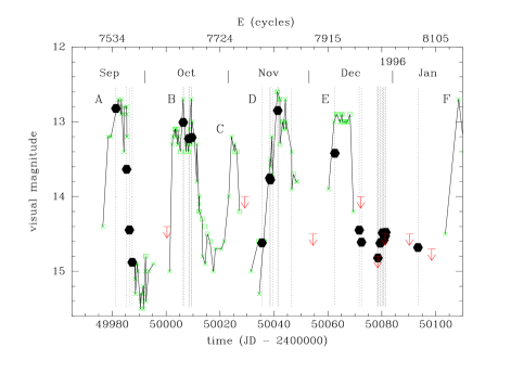
Figure 1: Visual lightcurve of EX Dra during the period September 1995 to January 1996, constructed from observations made by the AAVSO (crosses) and VSNET (open squares). Arrows indicate upper limits on the visual magnitude. Vertical dotted lines mark the epochs of our observations. $R$-band out-of-eclipse magnitudes from our dataset are shown as filled circles for illustration purposes.

Vertical dotted lines mark the epochs of our observations while filled circles show the corresponding $R$-band out-of-eclipse magnitudes. There were six recorded outbursts during this period (labeled from A to F in Fig. 1), with typical amplitudes of $\simeq 2.0$ mag, duration of $\simeq 10$ days, and average time between outbursts of $20\pm 3$ days. Outburst C was shorter ($\simeq 5$ days) and weaker ($\Delta m\simeq 1.5$ mag) than the others and, unfortunately, was not covered by our observations. The visual magnitude is typically $m_{v}\simeq 12.7$ at maximum and $m_{v}\simeq 15$ in quiescence. At the end of outbursts A and E the star went through a faint state (hereafter named low state) before recovering its usual quiescent level.

Our dataset frames eclipse lightcurves during most relevant phases through the outburst cycle: early rise to maximum (cycles 7812, 7813, 7817), late rise to maximum (7927), maximum light (7540, 7659, 7660, 7826 and 7827), end of maximum (7669, 7670, 7673, 7674 and 9583), early decline (7559, 7850), late decline (7564, 7970), low state (8002 to 8004), and quiescence (7569, 7798, 8007 to 8017, and 8074).

Individual lightcurves of EX Dra in quiescence are shown in Fig. 2.

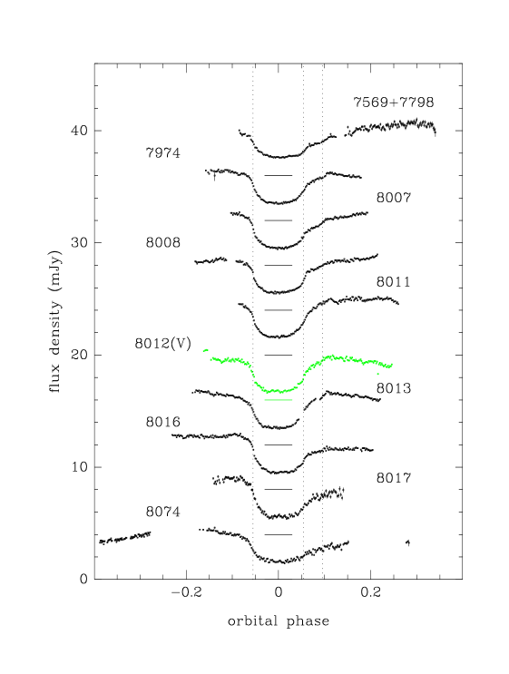
Figure 2: Lightcurves of EX Dra in quiescence. The curves are progressively displaced upwards by 4 mJy. Horizontal lines at mid-eclipse show the true zero level in each case. Vertical dotted lines mark the phases of ingress/egress of the bright spot and the egress of the white dwarf as measured in section 3.3. Labels indicate the cycle number.

Sharp changes in the slope reflect the occultation of a compact source at disc centre and of the bright spot at disc rim. The ingress of the central source and of the bright spot overlap in phase to form a unique sharp break in the slope. The egress of the central source is variable both in duration and in flux and sometimes is hardly visible (e.g., cycle 8074). The eclipses have a flat-bottomed, ‘U’ shape indicating that the eclipse is close from being total. There is no pronounced flickering (amplitude $\lower 2.15277pt\hbox{$\;\buildrel<\over{\sim}\;$}2.5$ per cent). In some of the lightcurves the flux level is the same before and after eclipse while others show a perceptible orbital hump prior to eclipse (usually interpreted as being the result of anisotropic emission from the bright spot) and a slow recovery from eclipse where the bright spot egress is hardly discernible.

Figure 3 shows lightcurves of EX Dra along the outburst cycle. The left panel shows the behaviour during rise and maximum light while the right panel shows the behaviour during decline and in the low state. The lightcurves were grouped by outburst phase. Only a subset of the outburst lightcurves are shown for clarity. The fact that, for a given outburst stage, the lightcurves of different outbursts have similar eclipse shapes and out-of-eclipse levels gives confidence that the observed sequence is representative of the general behaviour of EX Dra during outburst (at least for the epoch of our observations).

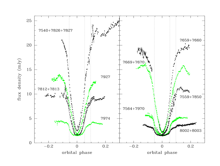
Figure 3: Lightcurves of EX Dra through the outburst cycle. Vertical dotted lines mark the phases of ingress/egress of the bright spot and the egress of the white dwarf as measured in section 3.3. Labels indicate the cycle number. The left panel shows lightcurves on the rise to maximum and at maximum while the right panel shows lightcurves during decline and in the low state. The quiescent lightcurve of cycle 7974 is shown in the left panel for reference.

Lightcurve 7812+7813 frames the early rise to maximum. The eclipse shape is asymmetric and mid-eclipse occurs after phase zero, indicating that the receding side of the disc is brighter. The mid-eclipse level and the total eclipse width are the same as in quiescence, showing that the brightening does not start in the outer disc regions. This is in agreement with the symmetric shape of the outbursts, with comparable rise and decline timescales (cf. Fig. 1), which is typical of inside-out outbursts (e.g., Cannizzo, Wheeler & Polidan 1986).

The eclipse profile changes during the rise to maximum, from the asymmetric ‘U’ shape eclipse of a compact central source plus the bright spot at disc rim to a more symmetric ‘V’ shape indicating the partial occultation of a bright extended disc. The total width of the eclipse increases during the rise (from 0.196 cycle in quiescence to about 0.22 cycle at lightcurve 7927 and larger at maximum) indicating that the disc radius also increases as the system approaches maximum light. A precise measurement of the total width of the eclipse at maximum light is precluded due to the limited phase coverage of the corresponding lightcurve.

The disc shrinks during decline (as indicated by the eclipse egress phase) until it reaches the quiescent radius close to the end of the outburst (lightcurve 7564+7970). The low state is characterized by an out-of-eclipse level $\simeq 15$ per cent lower than the typical quiescent level and by a fairly symmetric eclipse shape, corresponding to the eclipse of a compact source at the disc centre with little evidence of a bright spot at the disc rim. The mid-eclipse level of lightcurves 7564+7970 and 8002+8003 is the same, showing that the decrease in brightness at this stage is due to the fading of the light from the inner disc regions.

Flickering is much more pronounced in outburst than in quiescence. Flickers of an amplitude of $\simeq 10-15$ per cent can be seen in many lightcurves in outburst.

None of our outburst lightcurves resembles the flat-bottomed outburst lightcurve of Fiedler et al. (1997, see their fig. 6). Their outburst lightcurve is a factor of only $\simeq 2$ brighter than their typical quiescent lightcurve indicating that it corresponds to outbursts of lower amplitude than the ones sampled by our observations.

3.2 Revised ephemeris

The ingress feature of the white dwarf and of the bright spot overlap in quiescent lightcurves of EX Dra (Fig. 2). Since the bright spot ingress depends on the variable disc radius, the mid-ingress time is not a stable feature of the eclipse. We therefore adopted the same procedure of Fiedler et al. (1997) and used the mid-egress times of the white dwarf plus the inferred duration of its eclipse (see section 3.3) to obtain a revised ephemeris for the mid-eclipse times.

Mid-egress times were measured by computing the time of maximum derivative in a median-filtered version of the lightcurve (section 3.3). The uncertainty in determining mid-egress times depends on the time resolution and signal-to-noise of the lightcurve and is in the range $(1-2)\times 10^{-4}$ d. The barycentric correction and the difference between universal times (UT) and dynamical ephemeris time scales are smaller than the uncertainties in the measured timings and were neglected. The new heliocentric (HJD) times of the egress of the white dwarf are listed in Table 2 with corresponding cycle number and uncertainties (quoted in parenthesis).

Table 2: New eclipse timings.

cycle	white dwarf egress	(O$-$C)
	HJD (2 400 000 +)	(cycle)
7569	49987.4778 (2)	$+0.0009$
7974	50072.5023 (2)	$+0.0014$
8002	50078.3799 (2)	$-0.0017$
8003	50078.5900 (1)	$-0.0010$
8004	50078.8000 (1)	$-0.0006$
8007	50079.4296 (2)	$-0.0017$
8008	50079.6404 (1)	$+0.0025$
8011	50080.2700 (2)	$+0.0015$
8012	50080.4793 (1)	$-0.0016$
8013	50080.6893 (1)	$-0.0015$
8016	50081.3191 (1)	$-0.0015$
8017	50081.5290 (1)	$-0.0015$
8074	50093.4955 (1)	$-0.0010$

We assumed equal errors of $10^{-4}$ d for the timings of Fiedler et al. (1997) and combined them with the timings of Table 2 to obtain a least-squares linear fit with a reduced $\chi^{2}=13.8$ for 54 d.o.f. and a standard deviation of $\sigma=0.0019$ cycle. The residuals with respect to the linear ephemeris show a clear cyclical behaviour and can be well described by a sinusoidal function. Assuming a duration of the eclipse of the white dwarf of $\Delta t=0.0228$ d (section 3.3), the best-fit linear plus sinusoidal ephemeris for the mid-eclipse times is,

$$T_{mid}={\rm HJD}\;2\,448\,398.4530(\pm 1)+0.209\,936\,98(\pm 4)\,E+$$

$$+(8.2\pm 1.5)\times 10^{-4}\;\sin\left[2\pi\frac{(E-968)}{7045}\right]\;d\;\;\;,$$ (1)

with $\chi^{2}=2.7$ for 51 d.o.f. and $\sigma=0.0010$ cycle. Residuals with respect to the linear part of eq.(1) are listed in Table 2 and shown in Fig. 4. The sinusoidal term of eq.(1) is indicated in Fig. 4 as a dotted line.

Figure 4: The $(O-C)$ diagram for the eclipse mid-egress times calculated from the linear part of eq.(1). The timings of Fiedler et al. (1997) are plotted as open squares while those in Table 2 are shown as filled circles.

The amplitude (1.18 minutes) and timescale ($\simeq 4$ years) of the period variation are similar to the quasi-periodic orbital period changes found in many other eclipsing CVs (Warner 1995 and references therein) and are possibly related to a solar-like magnetic activity cycle in the secondary star (Applegate 1992; Richman, Applegate & Patterson 1994). It may also be possible that the period changes are due to a third body in the system, as suggested by Fiedler et al. (1997), if the variation proves to be strictly periodic. Regular observations of eclipse timings during the next decade are required in order to check the stability of the period of the variation and test the above hypotheses.

3.3 Binary parameters

3.3.1 Measuring eclipse phases

The ingress/egress phases of the occultation of the compact central source (hereafter CS) and of the bright spot (BS) by the secondary star provide information about the geometry of the binary system and the relative sizes of these components (e.g., Wood et al. 1986).

We used the lightcurves of the low state – where the effect of the BS is minimal on the eclipse shape – to measure the ingress and egress phases of the CS and to derive the width of its eclipse as well as the duration of its ingress/egress feature. The contact phases can be identified as rapid changes in slope visible in the lightcurves of the low state (Fig. 3) and were measured with the aid of a cursor on a graphic display of a median filtered version of the lightcurve. We defined $\phi_{c1},\phi_{c2}$ as those phases during which the CS disappears behind the secondary star and $\phi_{c3},\phi_{c4}$ as the phases corresponding to its reappearance from eclipse. The mid-ingress (egress) phases ($\phi_{ci},\phi_{ce}$) were computed as the phases at which half of the central source light is eclipsed and also as the phases of minimum (maximum) derivative in the lightcurve (e.g., Wood, Irwin & Pringle 1985).

Figure 5 illustrates the measurement procedure with the derivative for the combined lightcurve 8002+8003. The ingress/egress of the CS can be seen as those intervals for which the derivative curve is significantly different from zero.

Figure 5: Measuring the eclipse phases of the compact central source. (a) Lightcurve 8002+8003. (b) The median-filtered derivative of (a), multiplied by a factor 2. The dashed line is a spline fit to the extended and slowly varying eclipse of the disc. (c) The reconstructed central source lightcurve, shifted downwards by 1.5 mJy. (d) Lightcurve (a) after subtraction of the central source component, shifted downwards by 5 mJy. Dashed lines mark mid-ingress and mid-egress phases of the central source and dotted lines mark its four contact phases. Arrows indicate the beginning and end of the eclipse of the disc.

The width at half-peak intensity of these features yields a preliminary estimate of their duration. A spline function is fitted to the remaining regions in the derivative curve to remove the contribution from the extended and slowly varying eclipse of the disc. Estimates of the CS flux at ingress (egress) are obtained by integrating the flux in the spline-subtracted derivative curve between the first and second (third and fourth) contact phases. The lightcurve of CS is then reconstructed by assuming that the flux is zero between ingress and egress and that it is constant outside eclipse. The reconstructed CS lightcurve can be seen in Fig. 5(c) and the lightcurve after removal of the CS component is shown in Fig. 5(d).

The measured contact phases, mid-ingress and mid-egress phases of the CS from the lightcurves of the low state are collected in Table 3. The quoted mid-ingress/egress values are the average of both procedures described above and have an estimated error of 0.0005 cycle.

Table 3: Eclipse parameters from lightcurves of the low state.

cycle	$\phi_{c1}$	$\phi_{c2}$	$\phi_{c3}$	$\phi_{c4}$	$\phi_{ci}$	$\phi_{ce}$	$\Delta\phi$	$\phi_{0}\;\;\;$	$\Delta_{ci}$	$\Delta_{ce}$
8002	$-0.0595$	$-0.0515$	+0.0515	+0.0595	$-0.0545$	+0.0545	0.1090	0.0000	0.0080	0.0080
8003	$-0.0575$	$-0.0490$	+0.0515	+0.0600	$-0.0540$	+0.0540	0.1080	0.0000	0.0085	0.0085
8004V	$-0.0580$	$-0.0500$	+0.0515	+0.0600	$-0.0540$	+0.0550	0.1090	+0.0005	0.0080	0.0085
8002+8003	$-0.0595$	$-0.0515$	+0.0515	+0.0595	$-0.0540$	+0.0540	0.1080	0.0000	0.0080	0.0080
mean	$-0.0586$	$-0.0505$	+0.0515	+0.0598	$-0.0541$	+0.0544	0.1085	+0.0001	0.0081	0.0082
error	$\pm 0.0010$	$\pm 0.0010$	$\pm 0.0005$	$\pm 0.0003$	$\pm 0.0003$	$\pm 0.0005$	$\pm 0.0006$	$\pm 0.0003$	$\pm 0.0003$	$\pm 0.0003$

The duration of the CS eclipse (the eclipse of the disc centre) is defined as

$$\Delta\phi=\phi_{ce}-\phi_{ci}\;,$$ (2)

and the mid-eclipse phase (the inferior conjunction of the binary) is written as

$$\phi_{0}=1/2\>(\phi_{ce}+\phi_{ci})\;.$$ (3)

These quantities are collected in Table 3. The mean of the measurements from all lightcurves yields $\Delta\phi=0.1085\pm 0.0006$ cycle (=0.0228 d), where the quoted error is the standard deviation of the mean. Similarly, we have $\phi_{0}=+0.0001\pm 0.0003$ cycle, which indicates that the centre of the CS eclipse corresponds to phase zero. The difference between the first and second (third and fourth) CS contact phases yield the phase width of the CS ingress (egress), $\Delta_{\rm ci}$ ($\Delta_{\rm ce}$). These quantities are also listed in Table 3. A mean from all values of $\Delta_{\rm ci}$ and $\Delta_{\rm ce}$ yields $\Delta_{\rm cs}=0.0082\pm 0.0003$ cycle.

BS ingress/egress phases ($\phi_{bi},\phi_{be}$) were measured from the lightcurves in quiescence in which it was possible to simultaneously identify the eclipse of BS and the egress of CS. We measured the CS contact and mid-egress phases and used the derived value of $\Delta\phi$ to reconstruct the lightcurve of CS assuming that the flux and duration of its ingress feature are the same as in egress. Mid-ingress/egress phases of BS were measured in the lightcurves after removal of the CS component, which provide and unblended, clean view of the BS ingress feature (Fig. 6).

Figure 6: Measuring the eclipse phases of the bright spot. (a) Lightcurve 8007. (b) The reconstructed central source lightcurve, shifted upwards by 1 mJy. (c) Lightcurve (a) after subtraction of the central source component, shifted downwards by 3 mJy. (d) The derivative of lightcurve (c), multiplied by a factor 2 and shifted downwards by 2 mJy. Dashed lines mark the mid-ingress and mid-egress phases of the bright spot and dotted lines mark the four contact phases of the compact central source.

The eclipse parameters measured from the lightcurves in quiescence are listed in Table 4. The BS eclipse in lightcurve 7569 starts earlier and ends later than in the other lightcurves, indicating a relatively larger disc radius at this epoch (see section 3.3.2).

Table 4: Eclipse parameters from lightcurves in quiescence.

cycle	$\phi_{bi}$	$\phi_{be}$	$\phi_{c3}$	$\phi_{c4}$	$\phi_{ce}$	$\Delta_{ce}$
7569	$-0.061$	+0.099	+0.0480	+0.0620	+0.0550	0.014
8007	$-0.055$	+0.096	+0.0495	+0.0575	+0.0540	0.008
8008	$-0.055$	+0.096:	+0.0490	+0.0600	+0.0550	0.011
8012	$-0.056$	+0.095	+0.0490	+0.0600	+0.0545	0.011
8016+8017	$-0.054$	+0.096	+0.0510	+0.0580	+0.0540	0.007

3.3.2 Mass ratio, inclination and disc radius

Making the usual assumption that the secondary star fills its Roche lobe and given the duration of the eclipse of the central parts of the disc, $\Delta\phi$, there is a unique relation between the mass ratio $q=M_{2}/M_{1}$ and the binary inclination $i$ (Bailey 1979; Horne 1985). From Table 3, the width of the eclipse in EX Dra is $\Delta\phi=0.1085$. This gives the constraint $q>0.64$, with $q=0.64$ if $i=90\hbox{${}^{\circ}$}$.

When combined with the measured eclipse phases of the CS and BS, this relation gives a unique solution for $q$, $i$, and $R_{bs}/R_{L1}$, where $R_{bs}$ is the distance from disc centre to the BS (usually taken to be the disc radius) and $R_{L1}$ is the distance from disc centre to the inner lagrangian point L1 (e.g., Smak 1971; Cook & Warner 1984). Fig. 7(a) shows a diagram of ingress versus egress phases for the measurements of the CS and BS in Tables 3 and 4. Measurements of the CS ingress and egress are shown as the cluster of small diamonds around phases ($-0.054,+0.054$) in the lower portion of the diagram. Eclipse phases of BS are indicated by crosses.

Figure 7: Inferring the binary geometry from the ingress/egress phases of CS and BS. (a) Ingress-egress phases diagram. The observed phases of mid-ingress/egress of CS are marked with diamonds, those of BS with crosses. A diagonal dotted line depicts the line joining the component stars. Theoretical gas stream trajectories for three values of $q$ are plotted. The stream of matter passes through the position of BS for $q=0.72$. The squashed circles represent the accretion discs whose edges pass through the two distinct positions of the BS. For $q=0.72$, this yields disc radii of $R_{bs}=0.50$ and $0.56\;R_{L1}$. (b) The adopted geometry of the binary for $q=0.72$. The observed positions of CS and BS are shown with the theoretical gas stream trajectory and discs of radii $R_{bs}=0.50$ and $0.56\;R_{L1}$. The direction at which the bright spot is at maximum is indicated by an arrow.

Theoretical gas stream trajectories corresponding to a set of pairs $(i,q)$ are also shown. The trajectories were computed by solving the equations of motion in a coordinate system synchronously rotating with the binary, using a 4th order Runge-Kutta algorithm (Press et al. 1986) and conserving the Jacobi integral constant to one part in $10^{6}$. The correct mass ratio, and hence inclination, are those for which the calculated stream trajectory passes through the observed position of the bright spot. This yields $q=0.72\pm 0.06$ and $i=85^{+3}_{-2}$ degrees, where the uncertainties are taken from the standard deviation of the points about the trajectory of best fit. Fig. 7(b) shows the geometry of the binary system for $q=0.72$. For this mass ratio, the relative size of the primary Roche lobe is $R_{L1}/a=0.534\pm 0.009$, where $a$ is the orbital separation.

BS eclipse phases are clustered at two distinct positions along the best-fit stream trajectory. The squashed circles in Fig. 7(a) represent the accretion discs whose edges pass through these positions for the adopted mass ratio. This corresponds to disc radii of $R_{bs}/R_{L1}=(0.50\pm 0.01)$ and $(0.56\pm 0.01)$ with the bright spot making angles of, respectively, $\alpha_{bs}=20\hbox{${}^{\circ}$}\pm 1\hbox{${}^{\circ}$}$ and $16\hbox{${}^{\circ}$}\pm 1\hbox{${}^{\circ}$}$ with respect to the line joining both stars. Circles with these radii are depicted in Fig. 7(b). The larger disc radius comes from measurements of BS phases just after the end of an outburst (lightcurve 7569, end of outburst A) while the remaining points correspond to lightcurves well into quiescence (lightcurves 8007, 8008, 8012, 8016+8017). This result suggests that the accretion disc of EX Dra shrinks (by at least $\simeq 12$ per cent) during quiescence – a similar behaviour to that found in other dwarf novae (e.g., Smak 1984, 1991; Wood et al. 1989). The calculated radii are a factor of 2–3 larger than the radius expected for zero-viscosity discs, $R_{d}/R_{L1}\!=\!0.19$ (Flannery 1975), but are smaller than the radius expected for pressureless discs, $R_{d}/R_{L1}\!=\!0.66$ (Paczyński 1977).

Lightcurve 8074 gives the best phase coverage of the orbital hump in our dataset. The hump can be well described by a sinusoid of amplitude 0.6 mJy and maximum at orbital phase $-0.17\pm 0.01$ cycle. The direction of hump maximum (i.e., maximum visibility of the bright spot) is indicated in Fig. 7(b) by an arrow; it is clearly different from the radial direction of the bright spot. If the hump maximum is normal to the plane of the shock at the bright spot site then the shock lies in a direction between the stream trajectory and the edge of the disc, making an angle of $41\hbox{${}^{\circ}$}\pm 4\hbox{${}^{\circ}$}$ with the latter.

3.3.3 Masses and radii of the component stars

An estimate of the binary parameters of EX Dra may be obtained by combining the inferred mass ratio $q$ with the empirical main sequence mass-radius relation of Smith & Dhillon (1998),

$$R_{2}/R_{\odot}=\alpha\;\left(M_{2}/M_{\odot}\right)^{\beta}\;\;,$$ (4)

where $\alpha=0.91\pm 0.09$ and $\beta=0.75\pm 0.04$. The latter assumption seems reasonably well justified by the good quality of the fit to the measured masses of secondary stars in CVs and of field main sequence stars.

The primary-secondary mass diagram for EX Dra can be seen in Fig. 8. The constraints from the mass ratio and the empirical mass-radius relation are shown as thick solid lines. We also plotted lines corresponding to the mass functions for a radial velocity of the white dwarf of $K_{1}=167\;km\,s^{-1}$ (Fiedler et al. 1997) and for a radial velocity of the secondary star of $K_{2}=210\;km\,s^{-1}$ (Billington et al. 1996). The four relations are consistent at the 1-$\sigma$ level.

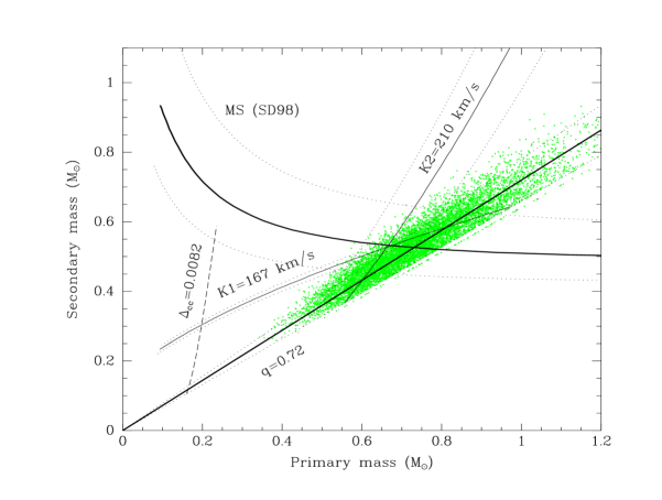
Figure 8: Primary-secondary star mass diagram for EX Dra. Thick solid lines show the constraints obtained from the inferred mass ratio of $q=0.72$ and the empirical mass-radius relation of Smith & Dhillon (1998) [SD98]. Solid lines illustrate the mass functions for a white dwarf radial velocity of $K_{1}=167\;km\,s^{-1}$ (Fiedler et al. 1997) and a radial velocity of the secondary star of $K_{2}=210\;km\,s^{-1}$ (Billington et al. 1996). Dotted lines indicate the 1-$\sigma$ limit on these relations. The gray cloud of points shows the confidence region and is the result of a $10^{4}$ points Monte Carlo simulation with the value of $q$ and the coefficients of the empirical mass-radius relation.

A Monte Carlo propagation code was used to estimate the errors in the calculated parameters. The values of the input parameters $q$ and ($\alpha,\beta)$ are independently varied according to Gaussian distributions with standard deviation equal to the corresponding uncertainties. The results, together with their 1-$\sigma$ errors, are listed in Table 5.

Table 5: Comparison of binary parameters.

parameter	reference
	this work	(1)	(2)	(3)
$q$	$0.72\pm 0.06$	0.80	0.75	0.73-0.97
$i$	$85\hbox{${}^{\circ}$}$ ($+3\hbox{${}^{\circ}$}$/$-2\hbox{${}^{\circ}$}$)	84.1	84.2	82.1
$M_{1}/M_{\odot}$	$0.75\pm 0.15$	0.66	0.75	0.70
$M_{2}/M_{\odot}$	$0.54\pm 0.10$	0.52	0.56	0.59
$R_{1}/R_{\odot}$	$0.011\pm 0.002$	0.011	0.013
$R_{2}/R_{\odot}$	$0.57\pm 0.04$		0.57	0.59
$a/R_{\odot}$	$1.61\pm 0.10$		1.63	1.58
$R_{d}/a$ (quies.)	$0.267\pm 0.004$	0.21	0.27
$\alpha_{bs}$ (quies.)	$20\hbox{${}^{\circ}$}\pm 1\hbox{${}^{\circ}$}$
$R_{L1}/R_{\odot}$	$0.85\pm 0.04$		0.85	0.82
$K_{1}\;(km\;s^{-1})$	$163\pm 11$	167	167	176
$K_{2}\;(km\;s^{-1})$	$224\pm 17$	210	223	210
$v_{2}\,\sin i\;(km\;s^{-1})$	$136\pm 9$	140		140
(1)= Billington et al. (1996), (2)= Fiedler et al. (1997),
(3)= Smith & Dhillon (1998).

The quoted $K_{1},K_{2}$ and $v\sin i$ are the predicted values of, respectively, the radial velocity of the primary and secondary stars and the secondary star rotational velocity; $a$ is the binary separation, and the remaining parameters are self-explanatory. The cloud of points in Fig. 8 was obtained from a set of $10^{4}$ trials using this code. The highest concentration of points indicates the region of most probable solutions. Table 5 also lists the estimated parameters of Billington et al. (1996), Fiedler et al. (1997) and Smith & Dhillon (1998). Our model of the EX Dra binary is in reasonably good agreement with the models independently derived by those authors from spectroscopic measurements.

We now turn our attention to the compact central source. An estimate of its diameter can be obtained from the duration of its ingress/egress feature in the lightcurve, $\Delta_{cs}$, using the approximate relations (Ritter 1980),

$$R_{cs}/a=\pi z(q)\;\Delta_{cs}\;\sin\theta\;,\;\;\;\;\;\cos\theta=\frac{a}{R_{2}}\cos i\;,$$ (5)

where $R_{cs}$ and $R_{2}$ are the radii of the central source and of the secondary star, respectively, and $z(q)$ is the distance (in units of $a$) from disc centre to the point tangent to the surface of the secondary that marks the beginning/end of the eclipse of CS (Baptista et al. 1989). $z(q)$ is a slow varying function and is usually close to unity. In our case, for $q=0.72$ we have $z=0.924$.

For the following exercise we adopted the value of $\Delta_{cs}=0.0082$ cycle inferred from the lightcurves of the low state (section 3.3.1). We note that the width of the CS ingress/egress feature is usually larger than this in the lightcurves in quiescence (see Table 4); from the mean $B$ lightcurve in quiescence of Fiedler et al. (1997) (see their fig. 7) we estimate a width of the egress feature of 0.010 cycle.

Assuming that the compact central source is the white dwarf, the substitution of Kepler’s third law into equation (5) yields a relation between the mass and the radius of the white dwarf than can be combined with the Hamada-Salpeter (1961) mass-radius relation (c.f. Nauenberg 1972) to eliminate $R_{cs}$ and solve for $M_{1}(q,\Delta_{cs})$ (e.g., Baptista et al. 1998). This relation (plotted in Fig. 8 as a dashed line) predicts unreasonably low white dwarf masses of $M_{1}\simeq 0.2\;M_{\odot}$, in clear disagreement with the results in Table 5. The discrepancy is not alleviated by the use of a mass-radius relation for hot white dwarfs (Koester & Shönberner 1986; Vennes, Fontaine & Brassard 1995), the inclusion of possible spherical distortion effects due to fast rotation of the white dwarf or the consideration of strong limb-darkening effects (Wood & Horne 1990), or by adopting the larger value of $\Delta_{cs}$ from the quiescent lightcurves. The measured $\Delta_{cs}$ is simply too large for a $\simeq 0.7\;M_{\odot}$ white dwarf in a binary with the orbital period of EX Dra. Together with the variability in flux and duration of the ingress/egress feature this leads to the conclusion that the observed compact central source is not a bare white dwarf.

The substitution of the parameters of Table 5 into equation (5) yields $R_{cs}(\Delta_{cs}=0.0082)=0.23\;a=0.037\;R_{\odot}=3.36\;R_{1}$. Therefore, the white dwarf in EX Dra seems surrounded by an extended, variable atmosphere or boundary layer of at least 3 times its radius. In this regard EX Dra is similar to the long period, eclipsing dwarf nova IP Peg – where the white dwarf seems to be wrapped in a thick boundary layer more than twice its radius (Wood & Crawford 1986) – and is clearly different from the short-period dwarf novae OY Car, Z Cha and HT Cas, where the central source seems to be a bare white dwarf (Wood & Horne 1990). This result suggests that different physical conditions may exist in the inner disc regions of the short period and of the long period dwarf novae, possibly related to the distinct mass accretion rates of these groups, although the statistics of eclipsing dwarf novae is still very low on both sides of the CV period gap. From the derived parameters, we predict a duration of the ingress/egress of the white dwarf of $\Delta_{wd}=0.0024\pm 0.0006$ cycle.

3.4 Distance estimates

The flux densities at mid-eclipse of the flat-bottomed lightcurves of the low state (Fig. 3) yield an upper limit to the contribution of the secondary star that can be used to set a lower limit on the distance to EX Dra (e.g., Baptista, Steiner & Cieslinski 1994).

We find $F_{\rm mid}(V)=0.79\pm 0.05$ mJy and $F_{\rm mid}(R)=1.56\pm 0.03$ mJy, where the quoted values are the median of the fluxes in the phase range ($-0.02,+0.02$) cycle and the uncertainties were derived from the median of the absolute deviations with respect to the median. This corresponds to an apparent magnitude of $V_{\rm mid}=16.66\pm 0.07$ mag and a color index of $(V-R)=+0.92\pm 0.07$ mag. We estimated a reddening of $E(B-V)=0.15\;{\rm mag}\;kpc^{-1}\;(A_{v}=4.8\times 10^{-4}\;{\rm mag}\;pc^{-1})$ for EX Dra from the galactic interstellar extinction contour maps of Lucke (1978), which gives a color excess of $E(V-R)=0.02$ mag for a distance of $D=290\;pc$ (see below). This leads to a corrected, intrinsic color index of $(V-R)_{0}=+0.90\pm 0.07$ mag.

A main sequence star with this color index has a spectral type M$0\pm 2$, an absolute magnitude of $M_{v}=9.2\pm 0.6$ mag and an effective surface temperature of $T_{\rm eff}=3850\pm 200\;K$ (Schmidt-Kaler 1982; Pickles 1985). This spectral type is in good agreement with that inferred from the spectroscopy by Billington et al. (1996) and Fiedler et al. (1997). With the assumption that the observed properties of the secondary star in EX Dra are similar to those of a normal main sequence star of same mass, we replace these values into the equation,

$$5\,\log D(pc)=V_{\rm mid}-M_{v}+5-A_{v}\,D(pc)\;\;\;,$$ (6)

to find a photometric parallax distance of $D_{MS}=(290\pm 80)\;pc$, where the quoted uncertainty is obtained from the propagation of errors in the input parameters and do not account for possible systematic errors. If we neglect the interstellar extinction, the inferred distance is reduced to $D=280\pm 80\;pc$. An alternative blackbody fit to the mid-eclipse fluxes including the interstellar extinction yields a solid angle of $\theta^{2}_{BB}=[(R_{2}/R_{\odot})/(D/kpc)]^{2}=3.8\pm 0.8$, an $T_{\rm eff}=3550\pm 250\;K$, and a distance of $D_{BB}=(290\pm 40)\;pc$. The measured mid-eclipse fluxes and the best-fit main sequence and blackbody spectra are shown in the upper panel of Fig. 9.

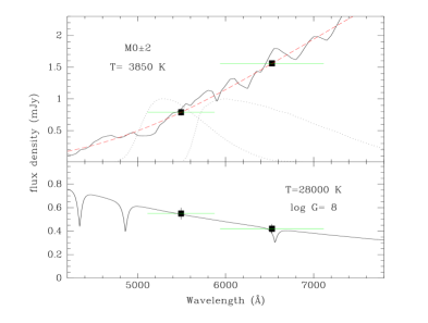
Figure 9: Top: $V$ and $R$ mid-eclipse fluxes (open squares) and best-fit main sequence (solid) and blackbody (dashed) spectra. Dotted curves show normalized response functions of the $V$ and $R$ passbands. Horizontal bars show the calculated flux of each model in the corresponding passband and marks the full-width half-maximum of each passband. Bottom: the measured fluxes of the central source and the best-fit white dwarf atmosphere model. The notation is the same as above.

Another distance estimate can be obtained from the $V$ and $R$ flux densities of the compact central source in the lightcurves of the low state, since we also have an estimate of the physical dimension of this source. The fluxes at egress, which are free from contamination of light from the bright spot, were obtained by integrating the derivative between the third and fourth contact phases (see section 3.3.1). We find $F_{cs}(V)=0.55\pm 0.05$ mJy and $F_{cs}(R)=0.42\pm 0.04$ mJy. We fitted the observed flux densities from synthetic photometry with white dwarf atmosphere models (Gänsicke, Beuermann & de Martino 1995) allowing for the effect of interstellar extinction as estimated above. The best-fit model has $T_{cs}=(28\pm 3)\times 10^{3}\;K,\>\log g=8$ and $\theta^{2}_{cs}=(3.3\pm 0.5)\times 10^{-3}$. The measured central source fluxes and best-fit white dwarf atmosphere model are shown in the lower panel of Fig. 9.

The corresponding distance depends on the geometry and effective emitting area of the central source as seen by an observer on Earth. A spherical central source has an effective area of $A_{sp}=\pi R^{2}_{cs}$ as projected onto the plane of the sky. In this case, if the inner disc is optically thin, both hemispheres of the central source are seen and a distance of $D=640\pm 50\;pc$ is obtained. If the inner disc is opaque the lower hemisphere of the central source is occulted and the distance is reduced to $D=450\pm 40\;pc$. Both values are in agreement with the lower limit derived from the contribution of the secondary star.

Alternatively, if we assume that the distance is $D=290\;pc$, the inferred $\theta^{2}_{cs}$ allow us to constrain the geometry of the central source. At this distance the effective area of the central source is reduced to 21 per cent of $A_{sp}$. Since the equatorial diameter of the central source is set by the width of its ingress/egress feature to be $2R_{cs}$, this implies that the polar diameter is significantly smaller than $R_{cs}$. Hence, the distance estimate from the flux of the secondary star and that from the flux of the central source can be reconciled if the central source has a toroidal shape with an equatorial diameter of $2\times 0.037\;R_{\odot}$ and a vertical thickness of $0.012\;R_{\odot}$ (if the inner disc is optically thin) or $0.024\;R_{\odot}$ (if the inner disc is opaque).

4 Summary

The results of the analysis of $V$ and $R$ high speed photometry of EX Dra in quiescence and through outburst can be summarized as follows:

1. During the period of the observations EX Dra showed outbursts with typical amplitudes of $\simeq 2.0$ mag, duration of $\simeq 10$ days, and average time between outbursts of $20\pm 3$ days. The observed amplitudes are larger than those found by Billington et al. (1996).

2. The lightcurves during outburst were grouped by outburst phase. The analysis of these lightcurves indicates that the outbursts do not start in the outer disc regions and, therefore, favours the disc instability model. The disc expands during the rise to maximum (as indicated by the increasing width of the eclipse) and shrinks during decline. The decrease in brightness at the later stages of the outburst is due to the fading of the light from the inner disc regions.

3. At the end of two outbursts the system was seen to go through a phase of lower brightness (named the low state), characterized by the fairly symmetric eclipse of a compact source at disc centre with little evidence of a bright spot at disc rim, and by an out-of-eclipse level $\simeq 15$ per cent lower than the typical quiescent level.

4. New eclipse timings were measured from the lightcurves in quiescence and a revised ephemeris was derived. The residuals with respect to the linear ephemeris show a clear cyclical behaviour and can be well described by a sinusoid of amplitude 1.2 minutes and period $\simeq 4$ years. This period variation is possibly related to a solar-like magnetic activity cycle in the secondary star.

5. Eclipse phases of the compact central source and of the bright spot were used to derive the geometry of the binary. By constraining the gas stream trajectory to pass through the observed position of the bright spot we find $q=0.72\pm 0.06$ and $i=85^{+3}_{-2}$ degrees.

6. The binary parameters were estimated by combining the measured mass ratio with the assumption that the secondary star in EX Dra obeys the empirical main sequence mass-radius relation of Smith & Dhillon (1998). The set of derived parameters in listed in Table 5.

7. The observed changes in the position of the bright spot with time suggest that the accretion disc shrinks during quiescence by at least $\simeq 12$ per cent.

8. The phase of hump maximum is distinct from the radial direction of the bright spot. If the hump maximum is normal to the plane of the shock at the bright spot site then the shock lies in a direction between the stream trajectory and the edge of the disc, making an angle of $41\hbox{${}^{\circ}$}\pm 4\hbox{${}^{\circ}$}$ with the latter.

9. The white dwarf seems surrounded by an extended, variable atmosphere or boundary layer of at least 3 times its radius. From the derived parameters, a duration of the ingress/egress of the white dwarf of $\Delta_{wd}=0.0024\pm 0.0006$ cycle is predicted.

10. The fluxes at mid-eclipse of the lightcurves of the low state yield an upper limit to the contribution of the secondary star and lead to a lower limit photometric parallax distance of $D_{MS}=290\pm 80\;pc$.

11. The fluxes of the central source are well fitted by a white dwarf atmosphere model with $T_{cs}=(28\pm 3)\times 10^{3}\;K,\>\log g=8$ and solid angle $\theta^{2}_{cs}=[(R_{cs}/R_{\odot})/(D/kpc)]^{2}=(3.3\pm 0.5)\times 10^{-3}$. For a spherical central source, this leads to a distance of $D=640\pm 50\;pc$ if the inner disc is optically thin. The distance estimates from the mid-eclipse fluxes and from the fluxes of the central source can be reconciled if the central source has a toroidal shape with an equatorial diameter of $2\times 0.037\;R_{\odot}$ and a vertical thickness of $0.012\;R_{\odot}$ (if the inner disc is optically thin) or $0.024\;R_{\odot}$ (if the inner disc is opaque).

The analysis of the set of lightcurves through outburst with eclipse mapping techniques yields an uneven opportunity to investigate the changes in the structure of an outbursting accretion disc and is the subject of another paper (Baptista & Catalán 1999, 2000).

References

- [1] Applegate J.H., 1992. ApJ, 385, 621
- [2] Bade N., Hagen H.-J., Reimers D., 1989. 23rd Eslab Symp. ESA SP-296, p.883
- [3] Bailey J., 1979. MNRAS, 187, 645
- [4] Baptista R., Catalán M.S., Horne K., Zilli D., 1998. MNRAS, 300, 233
- [5] Baptista R., Catalán M.S., 1999. Cataclysmic Variables: a 60th Birthday Symp. in honour of Brian Warner, eds. P. Charles et al., New Astronomy Reviews, in press (astro-ph/9905096).
- [6] Baptista R., Catalán M.S., 2000. in preparation
- [7] Baptista R., Jablonski F.J., Steiner J.E., 1989. MNRAS, 241, 631
- [8] Baptista R., Steiner J. E., Cieslinski D., 1994. ApJ, 433, 332
- [9] Barwig H., Fiedler H., Reimers D., Bade N., 1993. in Compact Stars in Binary Systems, IAU Symp. 165, ed. van Woerden H., p.89
- [10] Bell S.A., Hilditch R.W., Edwin R.P., 1993. MNRAS, 260, 478
- [11] Bessell M., 1983. PASP, 95, 480
- [12] Billington I., Marsh T.R., Dhillon V.S., 1996. MNRAS 278, 673
- [13] Cannizzo J.K., Wheeler J.C., Polidan R.S., 1986. ApJ, 301, 364
- [14] Cook M.C., Warner B., 1984. MNRAS, 207, 705
- [15] Fiedler H., Barwig H., Mantel K.-H., 1997. A&A, 327, 173
- [16] Flannery B.P., 1975. MNRAS, 170, 325
- [17] Gänsicke B.T., Beuermann K., de Martino D., 1995. A&A 303, 127
- [18] Horne K., 1985. MNRAS, 213, 129
- [19] Koester D., Shönberner D., 1986. A&A, 154, 125
- [20] Lamla E., 1982. in Landolt-Börnstein - Numerical Data and Functional Relationships in Science and Technology, New Series, Vol. 2, eds. K. Schaifers & H.H. Voigt, Springer-Verlag, Berlin
- [21] Lucke P.B., 1978. A&A, 64, 367
- [22] Massey P., Strobel K., Barnes J.V., Anderson E., 1988. ApJ, 328, 315
- [23] Massey P., Gronwall C., 1990. ApJ, 358, 344
- [24] Nauenberg M., 1972. ApJ, 175, 417
- [25] Paczyński B., 1977. ApJ, 216, 822
- [26] Pickles A.J., 1985. ApJS, 59, 33
- [27] Richman H.R., Applegate J.H., Patterson J., 1994. PASP, 106, 1075
- [28] Press W.H., Flannery B.P., Teukolsky S.A., Vetterling W.T., 1986. Numerical Recipes, Cambridge University Press, Cambridge
- [29] Ritter H., 1980. A&A, 86, 204
- [30] Smak J., 1971. Acta Astr., 21, 15
- [31] Smak J., 1984. Acta Astr., 34, 93
- [32] Smith D.A., Dhillon V.S., 1998. MNRAS, 301, 767
- [33] Schmidt-Kaler Th., 1982. in Landolt-Börnstein - Numerical Data and Functional Relationships in Science and Technology, New Series, Vol. 2, eds. K. Schaifers & H.H. Voigt, Springer-Verlag, Berlin
- [34] Vennes S., Fontaine G., Brassard P., 1995. A&A, 296, 117
- [35] Warner B., 1995. Cataclysmic Variable Stars, Cambridge Astrophysics Series 28, Cambridge University Press, Cambridge
- [36] Wood J.H., Crawford C.S., 1986. MNRAS, 222, 645
- [37] Wood J.H., Horne K., Berriman G., Wade R., O’Donoghue D., Warner B., 1986. MNRAS, 219, 629
- [38] Wood J.H., Horne K., Berriman G., Wade R., 1989. ApJ, 341, 974
- [39] Wood J.H., Horne K., 1990. MNRAS, 242, 609
- [40] Wood J.H., Irwin M.J., Pringle J.E., 1985. MNRAS, 214, 475