On dust-correlated Galactic emission in the Tenerife data

Abstract

Recently correlation analyses between Galactic dust emission templates and a number of CMB data sets have led to differing claims on the origin of the Galactic contamination at low frequencies. de Oliviera-Costa et al (1999) have presented work based on Tenerife data supporting the spinning dust hypothesis. Since the frequency coverage of these data is ideal to discriminate spectrally between spinning dust and free-free emission, we used the latest version of the Tenerife data, which have lower systematic uncertainty, to study the correlation in more detail. We found however that the evidence in favor of spinning dust originates from a small region at low Galactic latitude where the significance of the correlation itself is low and is compromised by systematic effects in the Galactic plane signal. The rest of the region was found to be uncorrelated. Regions that correlate with higher significance tend to have a steeper spectrum, as is expected for free-free emission. Averaging over all correlated regions yields dust-correlation coefficients of $180\pm 47$ and $123\pm 16$ $\mu$K /MJy sr^-1 at 10 and 15 GHz respectively. These numbers however have large systematic uncertainties that we have identified and care should be taken when comparing with results from other experiments. We do find evidence for synchrotron emission with spectral index steepening from radio to microwave frequencies, but we cannot make conclusive claims about the origin of the dust-correlated component based on the spectral index estimates. Data with higher sensitivity are required to decide about the significance of the dust-correlation at high Galactic latitudes and other Galactic templates, in particular H_α maps, will be necessary for constraining its origin.

1 Introduction

A small, but significant correlation of existing Cosmic Microwave Background (CMB) data with maps of Galactic dust emission has been detected. It is important to understand the origin, and hence the characteristics of any Galactic emission present in CMB maps with structure on angular scales relevant to CMB measurements. With such information, we can attempt to remove these contaminating emissions from the data, to be left with a pure CMB map.

Cross-correlating the COBE DMR maps with DIRBE far-infrared maps, Kogut et al (1996a,b) discovered that statistically significant correlations did exist at each DMR frequency, but that the frequency dependence was inconsistent with vibrational dust emission alone and strongly suggestive of additional dust-correlated free-free emission ($\beta_{ff}=-2.15$). A number of recent microwave observations have also shown that these correlations are not strongly dependent on angular scale. Different experiments ( DMR: Kogut et al. 1996b; 19GHz: de Oliviera-Costa et al. 1998; Saskatoon: de Oliviera-Costa et al. 1997; MAX5: Lim et al. 1996; OVRO: Leich et al. 1997), together give, with $95\%$ confidence, $-3.6<\beta_{radio}<-1.3$, consistent with free-free emission over the frequency range 15-50 GHz. However if the source of this correlated emission is indeed free-free, it is expected that a similar correlation should exist between $H_{\alpha}$ and dust maps. Several authors have found that these data sets are only marginally correlated (McCallough 1997 and Kogut 1997). Thus, most of the correlated emission appears to come from another source.

Draine and Lazarian (1998a,b) suggest that the correlated emission could originate from spinning dust grains. This model predicts a microwave emission spectrum that peaks at low microwave frequencies, the exact location of the peak depending on the size distribution of dust grains, and has a spectral index between -3.3 and -4, over the frequency range 15-50 GHz (Draine and Lazarian 1998b, Kogut 1999). The spectral indices obtained from various experiments do not seem to conform too well to the spinning dust model alone. However, recently de Oliveira-Costa et al (1999) (hereafter DOC99) claim to have found evidence of the spinning dust origin of DIRBE-correlated emission using the Tenerife 10 and 15GHz data. They find a rising spectrum from 10GHz to 15GHz, which is indicative of a spinning dust origin, as opposed to a free-free origin, for the dust-correlated Galactic foreground at these frequencies. In this paper, we use the most recent Tenerife data to show that the correlated emission is not necessarily indicative of spinning dust.

2 The data and Galactic templates

Tenerife is a double differencing experiment that takes data by drift scanning in right-ascension at each declination. Data are taken every $1\nobreak^{\circ}$ in RA and at intervals of $2.5\nobreak^{\circ}$ in Dec. We used the Tenerife 10GHz and 15GHz data in the region, $32.5\nobreak^{\circ}<$Dec$<42.5\nobreak^{\circ}$, and $0\nobreak^{\circ}<$RA$<360\nobreak^{\circ}$, with point sources subtracted and baselines removed. The Tenerife experiment has beams of FWHM $4.9\nobreak^{\circ}$ and $5.2\nobreak^{\circ}$ for the 10 and 15GHz experiments respectively, with a differencing angle of $8.1\nobreak^{\circ}$ between east and west positions on the sky to make up the final triple beam (Jones et al (1998)).

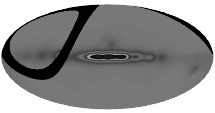
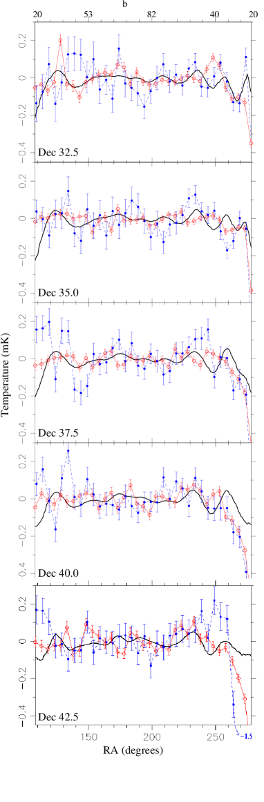
Figure 1 shows the patch of sky covered by the experiment in Galactic projection. Figure 2 shows the dust data and the Tenerife data at all the five declinations where data have been taken. We have extended the analysis presented in Gutierrez et al (1999) to also cover a region outside the high latitude range ($b>40\nobreak^{\circ}$) that they use to constrain CMB fluctuations. Therefore, the data we have used are different from that used in DOC99 as they did not extend the coverage of the raw data processing to be outside this range. This is one of the reasons we would expect differences between our results and those of DOC99. A great advantage of using the Tenerife data to constrain the spectral index of the dust-correlated component lies in the fact that similar angular scales and the same patch of the sky can be used. This is not the case when the correlation from different experiments are compared. Therefore, we have not used the two further declinations covered by the 15GHz data set (Decs $30\nobreak^{\circ}$ and $45\nobreak^{\circ}$), but not by the 10GHz data, avoiding any effect from features present in these declination strips. However, we have redone the calculations using these extra declinations and there was no significant difference with the results presented in this paper.

When looking at Figure 2, a difference between the two sides of the RA range, at almost all declinations is apparent. The rise (drop because of the double differencing) of the Galactic signal towards low Galactic latitude seen in the convolved dust maps on both sides of the RA range is only followed on one side by the Tenerife data. The Tenerife Galactic signal shows a stronger Galactic centre / anti-centre difference and a variation with declination which is different compared to the dust template with a particularly strong feature at Dec $42.5\nobreak^{\circ}$. Also note that the noisier 10GHz data show a wider spread toward low Galactic latitude, which does not appear systematically Galactic, at least when compared to the Galactic dust template. This may be due to a systematic error in the Tenerife data that is not fully represented by the error bars.

The Galactic templates used are the destriped DIRBE+IRAS $100\mu$m template of dust emission (Schlegel, Finkbeiner and Davis 1998), the 408MHz survey of synchrotron emission (Haslam et. al. 1981), and the 1420MHz survey of synchrotron emission (Reich $\&$ Reich, 1988, hereafter $R\&R$). We used the cleaned and destriped versions of the synchrotron emission maps by Lawson, Mayer, Osborne & Parkinson (1987).

Figure 1: The Figure shows the patch of sky covered by the Tenerife experiment in black, overlayed on the DIRBE template (smoothed to $5\nobreak^{\circ}$) to show the position of the Galactic plane.

Figure 2: The figure shows the Tenerife and dust data in the RA range that lies above the Galactic cut of $b>20\nobreak^{\circ}$, for all five declination strips. The filled circles and the dashed line represent the Tenerife 10GHz data, the empty circles and thin solid line represent the 15GHz data. The data have been binned every 5 points in RA. The corresponding $1\sigma$ error bars are shown. Units are mK. The thick solid line is the $100\mu m$ data convolved with the Tenerife beam. This data has been plotted in units of $0.13\times 1$ MJy/sr.

3 Correlation analysis and results

3.1 The method

Assuming that the microwave data consist of a super-position of CMB, noise and Galactic components, we can write

$$y=aX+x_{CMB}+n.$$

Here $y$ is a data vector of $N$ pixels, $X$ is an $N\times M$ element matrix containing $M$ foreground templates convolved with the Tenerife beam, $a$ is a vector of size $M$ that represents the levels at which these foreground templates are present in the Tenerife data, $n$ is the noise in the data and $x_{CMB}$ is due to the CMB convolved with the beam. The noise and CMB are treated as uncorrelated.

The minimum variance estimate of a is

$$\hat{a}=[X^{T}C^{-1}X]^{-1}X^{T}C^{-1}y,$$

with errors given by $\Delta\hat{a}_{i}=\Sigma_{ii}^{1/2}$ where $\Sigma$ is given as,

$$\Sigma=<\hat{a}^{2}>-<\hat{a}>^{2}=[X^{T}C^{-1}X]^{-1}.$$

$C$ above is the total covariance matrix (the sum of the noise covariance matrix and the CMB covariance matrix). The noise covariance matrix of the Tenerife data is taken to be diagonal, and the CMB covariance matrix is obtained through Monte-Carlo simulations with 10000 CMB realizations (this can of course be found analytically as well, as in DOC99). In all the above equations $X$ and $y$ are actually deviations of the corresponding quantities from the weighted mean with weights given by $C^{-1}$ (this is different to DOC99 who use the actual $X$ and $y$ in the analysis). It should be noted that there may be other components of emission present in the data so that the errors we consider here are only lower limits. Also, the templates that we are using may not be perfect and we do not account for possible uncorrelated structure in $C$. If there are other non-Gaussian components present in the data then the minimum variance estimate of $a$ will be incorrect.

3.2 Results

Listed in Table 1 are the correlation coefficients obtained for the Tenerife data sets and the $100\mu m$ DIRBE template, the Haslam, and the $R\&R$, with each Galactic template taken individually. Table 2 shows the correlation coefficients obtained when fits are done for two templates jointly. The DIRBE and Haslam correlations correspond to joint $100\mu m$-Haslam fits, whereas the $R\&R$ values correspond to joint $100\mu m-R\&R$ fits. $\Delta T=(\hat{a}\pm\Delta\hat{a})\sigma_{Gal}$ is the amplitude of fluctuations in temperature in the Tenerife data, that results from the correlation ($\sigma_{Gal}$ being the $rms$ deviation of the template map). The analysis is done for different Galactic cuts. Only positive Galactic latitudes are used in these tables as the Tenerife data do not extend below a $b$ of $-32\nobreak^{\circ}$.

From Table 1, we see that correlations with each of the three templates are detected with high significance. However these correlations fall off in significance towards higher Galactic latitudes. For comparison, the rms of the 10GHz data (after subtracting noise) for $b>20\nobreak^{\circ}$ is $181\pm 9\mu K$ (the error is due to a $5\%$ calibration uncertainty). If the templates are not significantly correlated with each other, one would conclude that 40% of the signal at 10 GHz is Galactic emission from Table 1. It should be noted that the correlation between the DIRBE and Haslam Galactic templates is significant for all Galactic cuts although if the dust and free-free emissions (or spinning dust) are 100% correlated then the Galactic emission would still only account for 50% of the total emission (assuming that all of the Galactic foregrounds present at this frequency are present in either the Haslam or DIRBE templates).

We also see that the DIRBE-correlated component has slightly higher significance than the Haslam or $R\&R$-correlated components near the Galactic plane for both the data sets. Away from the Galactic plane, at 10 GHz, the component correlated to the Haslam map becomes dominant (for $b>20\nobreak^{\circ}$) whereas at 15 GHz the DIRBE component remains dominant. However, there is almost no significant correlated emission beyond this Galactic cut.

3.3 Discussion

It is seen from Table 1 that individual correlations with dust do not show a rising (spinning dust) spectrum with significance between 10 and 15 GHz for any Galactic cut. From the joint $100\mu m-Haslam$ correlations (Table 2), we see that it appears as if there is some evidence for a rising spectrum of dust-correlated emission only for the $b>20\nobreak^{\circ}$ cut (as reported by DOC99). Spectral indices inferred from the correlation coefficients are listed in Table 3. Errors are small close to the Galactic plane. However, the values do not consistently agree with the spectral indices of any one of the three Galactic emission components, -2.8 for synchrotron, -2.1 for free-free and positive for spinning dust, for example +1 if the peak is at 20 GHz, that could be expected to be present as contaminating emissions in CMB data.

From Table 3 we see that the value of the spectral index inferred from the DIRBE-correlated component at 10 and 15 GHz is negative for most Galactic cuts (the correlations for $b>30\nobreak^{\circ}$ and $b>40\nobreak^{\circ}$ are not significant, so it was not possible to infer a spectral index). From the positive value of the spectral index for $b>20\nobreak^{\circ}$ DOC99 conclude that spinning dust is responsible for producing the major part of the DIRBE-correlated emission. However, since the spectral indices inferred for all other Galactic cuts are negative, a specific model of the spatial distribution of spinning dust would be required to explain the data. On the other hand it could also be that in the $b$-range where the Galactic signal in the Tenerife data drops the estimation of the spectral index becomes more sensitive to systematic effects we have not accounted for. To decide this we focus in on the $b>20\nobreak^{\circ}$ range and divide the data further. It should be noted that these spectral indices were found using the values for $\hat{a}$ and not $\Delta T$ as the beam sizes between the 10 and 15GHz data sets are slightly different giving rise to a lower expected $\Delta T$ (although the same relative level of contamination and hence $\hat{a}$) at 15 GHz than at 10 GHz which would systematically bias the values obtained.

When we examine the spectral indices obtained from the component correlated to the Haslam map at the two frequencies, we find that the values from the individual analysis are less negative than expected for synchrotron emission (Table 3). Joint correlation of the $100\mu$m dust and Haslam maps with the data result in spectral indices that are steeper than expected for synchrotron. This seems to imply that most of the emission in the 15GHz data that is correlated with the Haslam map is also correlated with the DIRBE maps (this is expected as the region that correlates lies close to the Galactic plane), leading to a much lower value of $\hat{a}$ for the synchrotron-correlated component than expected at 15GHz (and hence a much steeper spectrum). This may simply be because dust-correlated emission is more significant in the 15GHz data. Similarily since the Haslam -correlated emission is more significant at 10 GHz, the joint correlation method gives a lower value of $\hat{a}$ for the dust-correlated component and a correspondingly higher value for the synchrotron-correlated component. Being able to correct for this effect might therefore sort the systematic discrepancy. However, since we see this discrepancy with the synchrotron spectral index we should be wary of the dust template correlation as well.

If we now consider the DIRBE template to be an exact predictor for either spinning dust or free-free emission (so that all the features present in this template are present in the Tenerife data; as we are assuming when performing the correlation analysis) then the level of ‘contamination’ $a$ will be independent of the region tested. This means that each value of $a$ in Table 1 should be the same for the 10 and 15GHz data respectively. We can therefore take the variance of $a$ across the different regions analysed as a measure of the error in this method, and find that weighted mean and rms at 10 GHz and 15 GHz are 157 (20) and 122 (10) $\mu$K / (MJy sr^-1) respectively. This would correspond to a spectral index of $-0.6^{+0.5}_{-0.5}$.

3.4 Further study of the $b>20\nobreak^{\circ}$ cut region

We now divide the data into halves in RA, which gives two regions, one towards the Galactic centre and one towards the Galactic anticentre, at each declination. Repeating our analysis on these data we quantify the visual impression from Figure 2. Although the rise of the Galactic plane signal is equally strong in both regions of the dust template, we only find a significant correlation with the 10 and 15GHz data in the Galactic centre region, in spite of the fact that the noise errors in both regions are comparable. The results of this analysis are listed in table 4. It is seen that of the five declination stripes in the centre region only the three at higher declination are significantly correlated. The anticentre regions are found to be uncorrelated or even significantly anticorrelated in two stripes, which again demonstrates that the structure is not correlated rather than that our sensitivity is reduced when dividing the data. Again if we take the weighted mean and rms in the value of $a$ between declinations, we get 197 (66) and 157 (91) $\mu$K / (MJy sr^-1) for the centre regions at 10 and 15 GHz respectively, giving a spectral index of $-0.6^{+2.2}_{-2.8}$. The variation between declinations is high and the spectral index thus obtained is consistent with both free-free and spinning dust models.

We perform yet another split of the data in an attempt to identify the region where the correlation mainly comes from. It was found that the 20 pixels at lowest Galactic latitude of all declinations taken together (100 pixels) gave significant correlations, while the remaining pixels (750) gave no correlation (see table 5). Again the spectral index for dust-correlated emission is small and negative, while that for emission correlated to the Haslam map is steeper than expected. Since it is clear that the different declinations correlate differently, correlating them together is incorrect. Hence, shown also in table 5 are the values obtained for the same analysis on the 20 pixels at lowest Galactic latitude of each declination. Even though the signal to noise is much lower here, it is clear that the Galactic plane signal correlates with a free-free like spectral index while the rest of the pixels shows a significant anti-correlation with dust at 10 GHz for some declinations. The Galaxy correlates positively while the remaining regions correlate negatively or insignificantly. It is clear from analysing such splits that the correlation coefficients obtained when taking all declinations together as in tables 1 & 2 ($b>20\nobreak^{\circ}$) and in table 4 & 5, and which seem to indicate an almost flat or less negative spectral index between 10 and 15 GHz, are composed of regions that correlate with a negative spectral index and regions that do not correlate significantly at all. The anti-correlation, which occurs mostly in the 10GHz data, lowers the combined best fit $a$ value at that frequency, and hence raises the spectral index of dust-correlated emission. Note here that the high values of ’a’ obtained need not to be in contradiction to the level of free-free allowed by H_α as the detections are all close to the Galactic plane, where the level of free-free is expected to be high. We still see a large variance between the three declinations which correlate significantly. If we take the weighted mean and rms of the highest three declinations as indicative of a composite correlation, we get 313 (172) and 219 (83) $\mu$K / (MJy sr^-1) at 10 GHz and 15 GHz respectively, giving a spectral index of $-0.9^{+2.8}_{-2.2}$, again consistent with both free-free and spinning dust. Note that this value was obtained from the weighted average of three pairs of numbers shown in table 5, where each pair indicated a negative spectral index. The spectral index obtained simultaneously for the component correlated to the Haslam map is consistent within 1 $\sigma$ with the synchrotron spectral index.

Given that the dust templates correlate with the data only in a small part of the Tenerife patch above $b=20\nobreak^{\circ}$ we further test, how physically meaningful the detection is. This is important because the spectral index of a component in this method is inferred by assuming that the difference in the correlation amplitude between the frequencies is solely due to the change of emissivity of a single physical component and is not due to a spurious change in the strength of the correlation.

4 Sky rotations

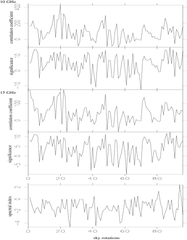
Another way to test for systematic errors in the method is to take random samples from the Galactic templates themselves as ”Monte Carlo” simulations. The advantage is that we can test against chance correlations with typical structure in the templates without having to understand the templates to a degree that would allow us to model this structure. Since the rise of the signal towards the Galactic plane clearly is a strong feature in the data and high Galactic latitude correlations are at best weak, we correlate to rotated / flipped maps in the northern and southern hemispheres, which all have the same orientation relative to the Galactic plane. Figure 3 shows $\hat{a}$ and its significance for 10 and 15 GHz, for the $b=20\nobreak^{\circ}$ Galactic cut, the Galactic centre region of all declination strips taken together, and the spectral indices derived from these values. We find that the real patch does not correlate most significantly at either frequency. Given the number of patches that correlate more significantly we conclude that the real correlation is at most typical and only due to the Galactic plane signal. Further we see that the 15 GHz real correlation although less significant than the neighbouring points has a higher value of $\hat{a}$. It seems that the real dust patch, although it does not represent the observed 15 GHz structure particularly well, happens to produces a high correlation amplitude. Indeed the real dust patch shows no strong features (low intensity rms), which explains the weak correlation and results in an overestimate of $\hat{a}$ at 15 GHz. An interesting point is that the mean spectral index which could be interpreted as the spectral index derived from correlations to typical Galactic plane dust signals, correlations which are about as significant as the real correlation, has a value of $-1.5\pm 1.2$, well consistent with free-free emission. The $rms$ variation in the value of the correlation coefficient at 10 and 15 GHz can be taken as an estimate of the error in $\hat{a}$ for the real patch. The error estimates obtained in this way range from about $20\%$ for $a$ at both 10 and 15 GHz for the $b>0$ Galactic cut, to $64\%$ and $30\%$ at 10 and 15 GHz respectively for the Galactic centre regions in the $b>20$ Galactic cut. As expected, the errors from sky-rotation increase with decreasing signal and size of the region and are very large for the individual declinations. Note that the lower Galactic cuts give the highest correlation with the highest significance for the real patch showing that the correlations there are not just due to aligned structure of the typical Galactic plane. The error estimates presented in this section are similar whether we include or exclude the rotated patches near the Galactic centre and anti-centre, where significantly different structure could be expected, though in the first case errors increase slightly for both 10 and 15 GHz. Henceforth we use results corresponding to the second case.

Since we have strong indication that the correlations between dust and the Tenerife data results only from the Galactic plane signal which will be similarly present in many physical components of Galactic emission we further investigate this particular feature of spatial distribution by modelling it in the next section.

Figure 3: The top four panels show the correlation coefficients and their significances when the 10 and 15 GHz data are correlated with different rotated patches of the dust template. These are joint correlations of the centre regions of all declinations combined, when the Haslam map is held fixed. The bottom panel shows the corresponding spectral indices. The first point in each panel corresponds to the real patch.

5 Galaxy modelling

A problem with the interpretation of the correlation results at different frequencies purely as a spectral dependence is that it neglects the possibility of variations in the shape of the Galaxy due to different components at different frequencies, and the resulting change of spatial alignment. For example, this method for obtaining the spectral index of correlated emission does not take into account the varying extent of the galaxy in the different data sets and template maps, so that the errors that we are quoting in the above tables might be too small and could be systematically wrong. If the Galaxy has a different spatial extent at 10 GHz, 15 GHz and 3 THz ($100~{}\mu$m), it will result in a higher or lower value for the overall correlation coefficient than is actually the case. We investigate this effect by modelling the spatial distribution of Galactic emission in the next section.

Figure 4: The Figure shows the FWHM of the Gaussian model for the Galaxy that gave the most significant correlation (or minimum $\chi^{2}$) plotted against the different data sets for the $b>20\nobreak^{\circ}$ Galactic cut and for Dec 40.0 (triangles) and Dec 37.5 (squares). The model was correlated with the Galactic centre regions of the data only.

Figure 5: Fitting the structure in the Tenerife data with the Gaussian model and the Galactic templates. Examples are shown for the 10 GHz data at Dec 42.5: (a) shows the best fit Gaussian model to the data and residuals (b) shows the Haslam (dashed) and dust (dotted) templates with amplitudes from the joint fit result and the thick dot-dashed line is the sum of the two (c) an equally acceptable fit, given the goodness of fit, is achieved when the spectra are normalised with the amplitudes of the templates at 15 GHz and are constrained to free-free and synchrotron spectral indices.

Figure 6: The Gaussian model (a) and the joint fit result (b) for the 15 GHz data at Dec 42.5

A significant correlation between the Tenerife data and the DIRBE dust template only occurs close to the Galactic plane where there is a rise in the overall Galactic signal. This rise may be frequency dependent if different physical components are present (for example free-free and synchrotron) so that care must be taken when comparing correlation results between different frequencies. We take a simple model of the Galaxy

$$S(b)=S_{\circ}\exp\left(-{b^{2}4\ln 2\over FWHM^{2}}\right)$$

where $b$ is the Galactic latitude, $S$ is the amplitude and $FWHM$ is the full width half maximum of the Gaussian model for the Galactic plane. The value of $S_{\circ}$ is arbitrary as it will only scale the estimate for $a$ for the various correlation results and not affect the relative value between models with different width. Each model is then convolved with the appropriate experimental beam, and correlated with the data, while varying FWHM.

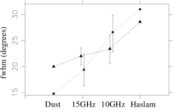
Figure 4 shows the widths of the Galactic models which correlated best with the data and the Galactic templates for the two declination strips in the centre region which do show convincing correlation. Two strips showed no significant correlation between the data and the templates, and Dec $=42.5\nobreak^{\circ}$ has the strong feature at 10 GHz, which is also incompatible with the templates. It can be seen that the most significant correlation between the dust/Haslam template and the model occurs with Galactic models of different sizes (FWHM), which are also different from the sizes obtained for the 10 and 15GHz data. However there seems to be a clear trend of decreasing width with increasing frequency compatible with more synchrotron emission at 10 GHz and more dust-correlated structure at 15 GHz. The combined fit to all declination stripes simultaneously also shows this expected trend of increasing Galactic width with wavelength. If this systematic change is real we might be able to fit for two distinct components with different width and spectral index. Although our fits of a single Gaussian component are all well acceptable the quality of the data is however not good enough to fit for two such components, if they are present independently of templates.

In Figure 4 the points for the dust correlations lie closer to the 15 GHz points than to the 10 GHz points, implying a better match of the Galactic shape for 15 GHz. When correlating the dust template to the data, the significance of any correlation will drop and $\hat{a}$ will change systematically, because the structure at each frequency is different. When correcting for this mismatch, assuming that the correlated component we are looking for has identical appearance at any frequency, we find that the correlation amplitudes for both 10 and 15 GHz shift upwards. However the 10 GHz amplitude, because of the larger difference in size with dust, gets a larger shift, which results in a drop of the spectral index for the dust-correlated emission by typically about 0.2. Taking this effect of mismatched structure into account for the Haslam correlations results in a less steep spectral index, which is more consistent with synchrotron emission.

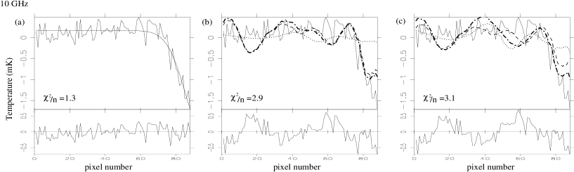
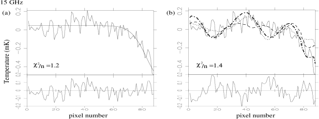
When we subtract the best fitting Galactic models from the data and the templates no correlations remain between the residuals, neither between the data and the templates nor between the templates, showing again that any correlation is only due to the Galactic plane signal, which we are able to model. Figure 5 shows these best fit models for the 10 and 15GHz data, for Dec 42.5, and the residuals. The fit achieved by the single component Gaussian model is indeed good and in fact better than the joint correlation fit, which we show for comparison. Further we find that since the joint fit to the 10 GHz data is rather poor in terms of goodness of fit, synchrotron and free-free components with the expected spectral indices (-2.8 and -2.1) can be fitted with an almost similar goodness of fit, based on the reduced $\chi^{2}$. When the same is done for the other declinations the goodness of fit is generally better for both the joint fit as well as the model fitting. Further in the other declinations also we generally find equally acceptable fits for a dust-correlated component which is constrained to give a free-free spectral index.

6 Template errors

Another yet unaccounted source of error is an intrinsic error in the dust template itself, which can be instrument noise or data reduction errors due to point source subtraction etc., but also systematic variations in the dust emissivity, which might not be followed in the same way by the components at 10 and 15 GHz. Note that the DIRBE maps at different frequencies are correlated with each other to not more than $95\%$. If we assume that there is a $5\%$ Gaussian error in the flux at $100~{}\mu$m due to these errors we can model this effect to quantify any change that would occur in the correlation. To do this we added a $5\%$ error in the flux (on the Tenerife angular scales) to the maps and calculated the new values of $a$. We performed 300 Monte-Carlo simulations and found that there was a systematic drop in $a$ for the 10 and 15 GHz data by factors of $1.6$ and $1.4$ respectively, when the centre regions of all declinations were taken together for the $b>20\nobreak^{\circ}$ cut (similar values are obtained when the entire $b>20\nobreak^{\circ}$ region is taken). Turning this effect around for the real data, assuming that there is an intrinsic $5\%$ error present in the template map, we need to increase the values of $a$ given in the tables by these factors. The value of $a$ at 10 GHz has to be increased relative to 15 GHz, which results in a significantly steeper spectral index, again more consistent with free-free emission. However, it should be noted that we do not have error maps for the templates at present and thus in this current paper we have not attempted a quantitative evaluation of this effect Presumably template errors, given that we have an idea of the likely causes, will be greater towards the Galactic plane. Since we have found that the only correlations we have to report result for pixels close to the Galactic centre, this will be an important source of systematic error.

7 Conclusions

Spinning dust emission can be identified and discriminated from free-free emission if indications for a peak in the emission spectrum can be found at low microwave frequencies, which are probed by the Tenerife experiment. A rising spectrum between 10 and 15 GHz can be taken as a prediction of the spinning dust hypothesis, although the exact location of the emission peak depends on details of the model. Tentative evidence for a turnover in the spectrum of the Galactic dust-correlated microwave component between 10 and 15 GHz has been presented by DOC99. We however find that the spectral index of dust-correlated emission is negative for all Galactic cuts except for the $b>20\nobreak^{\circ}$ cut. The Galactic signal, and with it the significance of the correlation, decreases with increasing Galactic latitude, and no correlations are detected in the higher Galactic latitude regions of $b>30\nobreak^{\circ}$. The variance in the value of $\hat{a}$ between regions with different Galactic cuts is rather large. We further find that the correlation detected in the $b>20\nobreak^{\circ}$ region comes only from a small number of pixels at low Galactic latitude and towards the Galactic centre, where signal from the Galactic plane is present. This correlation shows a free-free like spectral index, whereas the rest of the region was found to be uncorrelated, or even significantly anticorrelated.

Using sky rotations we show that the correlation we see at $b>20\nobreak^{\circ}$ is only an alignment of structure due to the rise of the Galactic plane signal. Employing a simple model for this structure we were able to demonstrate that the spatial distribution of Galactic emission is in fact different in the templates and in the data, giving rise to a systematic error. We were also able to show that this simple model of the Galaxy fits the data generally better than the templates. Further, modelling a Galactic free-free component, which correlates with the dust template, generally yields an equally acceptable fit to the data. Another significant systematic effect arises due to intrinsic errors in the templates, and all these effects cause a misleading increase in the inferred spectral index of the dust-correlated component between 10 and 15 GHz.

A comparison of our results with other experiments is presented in Figure 7. Here the data points for the Tenerife experiment, obtained by taking a weighted average of all detections (all regions of all Galactic cuts, joint analyses) with errors taken from the sky rotations, correspond to values of $180\pm 47$ and $123\pm 16$ $\mu$K /MJy sr^-1 at 10 and 15 GHz respectively. Note that the 10GHz point on the plot is significantly higher, as compared to that plotted in DOC99 and the value quoted in our table 2 This is because this region consists of parts that are correlated as well as parts that do not correlate or even anticorrelate, as in the case of the 10GHz data. Here, since we are focussing only on the regions that correlate (these regions are the same for both 10 and 15 GHz data and have been found to lie close to the Galactic plane), the value is significantly higher. Note that the high values of $a$ that we get need not be in contradiction to the typical level of free-free allowed by $H_{\alpha}$ maps of other regions as our detections are close to the Galactic plane, where the level of Galactic emission is expected to be high.

Figure 7: Summary of our results on the dust-correlated (top panel) and synchrotron-correlated (bottom panel) emission compared to results from other experiments (COBE DMR-filled circles, 19GHz-empty triangle, OVRO-filled triangle, Saskatoon-filled square). The straight lines represent synchrotron (solid), free-free (dotted) and vibrational dust (dashed) spectral indices. The thick solid curve shows a combination of free-free emission with a small spinning dust contribution with a peak at 15 GHz in an attempt to fit all the data. This fit appears acceptable, as does the single free-free component fit, but it should be kept in mind that the data from different experiments might not be directly comparable, since they were taken on different angular scales and towards different regions of the sky. The Tenerife data points are an average derived from our various results, see text for details.

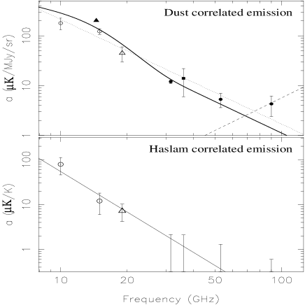
The spectral index for dust-correlated emission as deduced from the 10 and 15 GHz points is less negative (by about $1\sigma$) than expected for free-free emission. The spectral index deduced simultaneously from synchrotron-correlated emission is systematically steeper than expected. This could be attributed to the effects that we have identified and which have all been shown to influence the correlation in the same direction. Note also that in this plot only the Tenerife and COBE DMR points, at different frequencies, each represent data which probe the same angular scales and were taken with the same sky coverage. Inferring a spectral index by comparing different experiments assumes that the Galactic component is traced by a given fixed template and does not depend on parameters which vary over the sky, but our analysis of the Tenerife data shows large variations of Galactic correlation with the sky region.

With the present analysis of Tenerife data we are not able to make a firm claim about the origin of the dust-correlated component, since we do not find convincing support for a spinning dust component. This does not have to rule out this hypothesis, since environmental conditions or grain sizes, which affect the position of the spectral peak, could change systematically with location on the sky, particularly in the transition region between low and high Galactic latitude. The spatial variation in the correlation amplitude and the possibility of the presence of some spinning dust emission along with free-free emission need to be dealt with. The separation task is difficult for two reasons. Firstly neither the frequency dependence nor the spatial distribution of any of the Galactic components at low microwave frequencies is particularly well known. And further we would expect these components to be correlated, since we find their templates to be correlated, at least at low Galactic latitudes. The combination of the results from the other experiments, shown in Figure 7, might not be strongly constraining, but nevertheless, does not give conclusive evidence for spinning dust emission either, without an expectation of the amplitude of free-free emission based on dust-correlated H_α emission.

In order to make more reliable inferences, a pixel by pixel separation of components would have to be performed, using the Maximum Entropy method for example. In a forthcoming paper we shall perform such a separation incorporating information about spinning dust. Also, including other data at frequencies lower than 10 GHz and adding other templates of Galactic emission such as the $H_{\alpha}$ maps from the Wisconsin H-Alpha mapper (Tufte, Reynolds and Haffner 1998) would be useful.

Table 1: Individual correlations for the Tenerife data. $\hat{a}$ is the correlation coefficient, and has units $\mu K(MJy/sr)^{-1}$ for the $100\mu$m template, and $\mu K/K$ for the Haslam and $R\&R$ templates.

		10GHz		15GHz
b	Template	$\hat{a}\pm\Delta(\hat{a})$	$\Delta T\mu K$	$\hat{a}\pm\Delta(\hat{a})$	$\Delta T\mu K$
$b>0\nobreak^{\circ}$	$100\mu m$	$214\pm 0$	$6435\pm 13$	$119\pm 0$	$3430\pm 6$
	Has	$591\pm 1$	$5850\pm 12$	$333\pm 1$	$3189\pm 6$
	$R\&R$	$26140\pm 64$	$4684\pm 11$	$14176\pm 33$	$2476\pm 5$
$b>5\nobreak^{\circ}$	$100\mu m$	$209\pm 1$	$3127\pm 10$	$123\pm 0$	$1770\pm 5$
	Has	$545\pm 2$	$2617\pm 9$	$323\pm 1$	$1502\pm 4$
	$R\&R$	$17324\pm 86$	$1773\pm 9$	$10790\pm 41$	$1077\pm 4$
$b>10\nobreak^{\circ}$	$100\mu m$	$268\pm 1$	$1918\pm 11$	$136\pm 1$	$967\pm 4$
	Has	$431\pm 3$	$1422\pm 9$	$259\pm 1$	$839\pm 4$
	$R\&R$	$13209\pm 98$	$1079\pm 8$	$8654\pm 47$	$692\pm 4$
$b>15\nobreak^{\circ}$	$100\mu m$	$259\pm 9$	$199\pm 7$	$132\pm 4$	$106\pm 3$
	Has	$142\pm 5$	$161\pm 6$	$81\pm 3$	$90\pm 3$
	$R\&R$	$4727\pm 148$	$207\pm 6$	$2883\pm 84$	$125\pm 4$
$b>20\nobreak^{\circ}$	$100\mu m$	$131\pm 21$	$41\pm 7$	$140\pm 13$	$43\pm 4$
	Has	$71\pm 6$	$70\pm 6$	$29\pm 4$	$28\pm 4$
	$R\&R$	$2294\pm 256$	$54\pm 6$	$1514\pm 165$	$35\pm 4$
$b>30\nobreak^{\circ}$	$100\mu m$	$18\pm 38$	$4\pm 8$	$32\pm 26$	$6\pm 5$
	Has	$20\pm 8$	$20\pm 8$	$7\pm 4$	$6\pm 4$
	$R\&R$	$897\pm 390$	$17\pm 7$	$379\pm 255$	$7\pm 5$
$b>40\nobreak^{\circ}$	$100\mu m$	$39\pm 43$	$8\pm 8$	$13\pm 30$	$2\pm 6$
	Has	$18\pm 10$	$14\pm 8$	$10\pm 7$	$8\pm 5$
	$R\&R$	$964\pm 432$	$18\pm 8$	$531\pm 304$	$10\pm 5$

Table 2: Joint correlations for the Tenerife data. $\hat{a}$ is the correlation coefficient, and has units $\mu K(MJy/sr)^{-1}$ for the $100\mu$m template, and $\mu K/K$ for the Haslam and $R\&R$ templates.

		10GHz		15GHz
b	Template	$\hat{a}\pm\Delta(\hat{a})$	$\Delta T\mu K$	$\hat{a}\pm\Delta(\hat{a})$	$\Delta T\mu K$
$b>0\nobreak^{\circ}$	$100\mu m$	$151\pm 1$	$4535\pm 36$	$114\pm 1$	$3281\pm 19$
	Has	$191\pm 3$	$1895\pm 33$	$16\pm 2$	$157\pm 18$
	$R\&R$	$6829\pm 90$	$1224\pm 16$	$1645\pm 52$	$287\pm 9$
$b>5\nobreak^{\circ}$	$100\mu m$	$154\pm 1$	$2311\pm 21$	$116\pm 1$	$1669\pm 10$
	Has	$171\pm 4$	$821\pm 19$	$23\pm 2$	$106\pm 10$
	$R\&R$	$5587\pm 99$	$572\pm 10$	$1405\pm 54$	$140\pm 5$
$b>10\nobreak^{\circ}$	$100\mu m$	$238\pm 3$	$1704\pm 20$	$136\pm 1$	$961\pm 10$
	Has	$64\pm 5$	$213\pm 17$	$0\pm 3$	$0\pm 10$
	$R\&R$	$1701\pm 140$	$139\pm 11$	$394\pm 79$	$31\pm 6$
$b>15\nobreak^{\circ}$	$100\mu m$	$200\pm 10$	$154\pm 7$	$110\pm 5$	$88\pm 4$
	Has	$94\pm 6$	$106\pm 7$	$26\pm 4$	$29\pm 4$
	$R\&R$	$3393\pm 211$	$148\pm 9$	$1858\pm 140$	$81\pm 6$
$b>20\nobreak^{\circ}$	$100\mu m$	$67\pm 22$	$21\pm 7$	$122\pm 14$	$38\pm 4$
	Has	$65\pm 7$	$64\pm 6$	$12\pm 4$	$11\pm 4$
	$R\&R$	$1983\pm 288$	$47\pm 7$	$726\pm 203$	$17\pm 5$
$b>30\nobreak^{\circ}$	$100\mu m$	$-16\pm 40$	$-3\pm 8$	$18\pm 28$	$4\pm 6$
	Has	$21\pm 8$	$19\pm 7$	$6\pm 5$	$5\pm 5$
	$R\&R$	$1087\pm 455$	$20\pm 8$	$291\pm 304$	$5\pm 5$
$b>40\nobreak^{\circ}$	$100\mu m$	$0\pm 49$	$0\pm 10$	$-21\pm 37$	$-4\pm 7$
	Has	$18\pm 11$	$14\pm 9$	$13\pm 8$	$10\pm 6$
	$R\&R$	$1245\pm 576$	$23\pm 10$	$842\pm 421$	$15\pm 8$

Table 3: Spectral indices obtained from individual and joint correlations. No number is given when the correlation is insignificant.

	Individual analysis		joint analysis
cut	dust	Haslam	dust	Haslam
$b>0\nobreak^{\circ}$	$-1.45^{+0.01}_{-0.01}$	$-1.41^{+0.01}_{-0.01}$	$-0.69^{+0.04}_{-0.04}$	$-6.11^{+0.34}_{-0.37}$
$b>5\nobreak^{\circ}$	$-1.31^{+0.01}_{-0.01}$	$-1.29^{+0.02}_{-0.02}$	$-0.70^{+0.04}_{-0.04}$	$-4.95^{+0.27}_{-0.28}$
$b>10\nobreak^{\circ}$	$-1.67^{+0.03}_{-0.03}$	$-1.25^{+0.02}_{-0.03}$	$-1.38^{+0.05}_{-0.05}$	$-$
$b>15\nobreak^{\circ}$	$-1.66^{+0.16}_{-0.16}$	$-1.38^{+0.17}_{-0.18}$	$-1.47^{+0.23}_{-0.24}$	$-3.17^{+0.52}_{-0.56}$
$b>20\nobreak^{\circ}$	$0.16^{+0.65}_{-0.60}$	$-2.21^{+0.54}_{-0.56}$	$1.48^{+1.35}_{-1.00}$	$-4.17^{+1.00}_{-1.25}$
$b>30\nobreak^{\circ}$	$-$	$-2.56^{+2.35}_{-2.95}$	$-$	$-3.09^{+2.68}_{-5.21}$
$b>40\nobreak^{\circ}$	$-$	$-1.45^{+3.31}_{-4.06}$	$-$	$-0.80^{+3.51}_{-3.53}$

Table 4: Joint correlations obtained for data at different declinations when the data at each declination are divided into two halves, one half being towards the Galactic centre (marked C) and the other towards the anticentre (marked AC).

		10GHz			15GHz
region	number of pixels	$dust$	$Haslam$	$\chi^{2}$	$dust$	$Haslam$	$\chi^{2}$
all Decs, C	426	$160\pm 33$	$89\pm 9$	$856$	$182\pm 22$	$27\pm 7$	$530$
all Decs, AC	424	$-80\pm 32$	$15\pm 10$	$481$	$43\pm 21$	$-50\pm 6$	$469$
Dec 42.5, C	88	$225\pm 95$	$341\pm 27$	$259$	$261\pm 55$	$78\pm 18$	$122$
Dec 42.5, AC	87	$-185\pm 73$	$29\pm 19$	$107$	$24\pm 43$	$-12\pm 12$	$88$
Dec 40.0, C	86	$276\pm 56$	$74\pm 33$	$94$	$225\pm 41$	$83\pm 22$	$93$
Dec 40.0, AC	86	$-148\pm 55$	$-12\pm 18$	$94$	$21\pm 34$	$-1\pm 12$	$79$
Dec 37.5, C	85	$177\pm 50$	$89\pm 22$	$100$	$173\pm 32$	$25\pm 14$	$69$
Dec 37.5, AC	85	$36\pm 52$	$37\pm 17$	$100$	$17\pm 32$	$-5\pm 10$	$79$
Dec 35.0, C	84	$75\pm 74$	$50\pm 13$	$85$	$72\pm 45$	$12\pm 10$	$86$
Dec 35.0, AC	84	$0\pm 54$	$-8\pm 21$	$86$	$17\pm 33$	$-13\pm 10$	$106$
Dec 32.5, C	83	$215\pm 94$	$-12\pm 20$	$57$	$-77\pm 69$	$38\pm 15$	$71$
Dec 32.5, AC	82	$-75\pm 92$	$7\pm 24$	$79$	$128\pm 43$	$13\pm 11$	$89$

Table 5: The following table shows the correlation coefficients $\hat{a}\pm\Delta(\hat{a})$ obtained when the 20 pixels with lowest Galactic latitude in the Galactic centre region in each declination are correlated with the corresponding structure in the template maps, and those obtained when the remaining pixels are correlated. All these are joint fits.

		10GHz			15GHz
region	number of pixels	$dust$	$Haslam$	$\chi^{2}$	$dust$	$Haslam$	$\chi^{2}$
all Decs	100	$178\pm 44$	$111\pm 14$	$479$	$167\pm 31$	$18\pm 11$	$159$
all Decs	750	$-52\pm 27$	$22\pm 8$	$821$	$29\pm 19$	$47\pm 51$	$808$
Dec 42.5	20	$1148\pm 374$	$279\pm 49$	$40$	$466\pm 141$	$24\pm 29$	$24$
Dec 42.5	155	$-147\pm 57$	$37\pm 17$	$187$	$54\pm 35$	$-14\pm 11$	$174$
Dec 40.0	20	$264\pm 90$	$48\pm 10$	$26$	$177\pm 59$	$35\pm 65$	$24$
Dec 40.0	152	$-75\pm 47$	$0\pm 16$	$160$	$26\pm 30$	$10\pm 10$	$139$
Dec 37.5	20	$315\pm 144$	$163\pm 92$	$19$	$217\pm 75$	$64\pm 54$	$10$
Dec 37.5	150	$10\pm 46$	$51\pm 15$	$180$	$6\pm 29$	$1\pm 8$	$129$
Dec 35.0	20	$23\pm 121$	$53\pm 21$	$20$	$34\pm 77$	$3\pm 18$	$23$
Dec 35.0	148	$21\pm 48$	$14\pm 15$	$150$	$7\pm 30$	$-6\pm 8$	$170$
Dec 32.5	20	$152\pm 200$	$9\pm 58$	$18$	$32\pm 152$	$8\pm 42$	$10$
Dec 32.5	145	$34\pm 73$	$0\pm 17$	$125$	$79\pm 39$	$18\pm 9$	$155$

References

- [1] de Oliviera-Costa, A. et al. 1997, ApJ, 482, L17
- [2] de Oliviera-Costa, A. et al. 1998, ApJ, 509, L9
- [3] de Oliviera-Costa, A. et al. 1999, Submitted to ApJ (astro-ph/9904296) (DOC99)
- [4] Draine, B.T., and Lazarian, A. 1998a, ApJ, 494, L19
- [5] Draine, B.T., and Lazarian, A. 1998b, ApJ, 508, 157
- [6] Gutierrez, C.M. et al. 1999, astro-ph/9903196
- [7] Haslam, C.G.T., et al 1981, , 100, 209
- [8] Jones, A.W. et al. 1998, MNRAS, 294, 582
- [9] Kogut, A. et al. 1996a, ApJ, 460, 1
- [10] Kogut, A. et al. 1996b, ApJ, 464, L5
- [11] Kogut, A., 1997, AJ, 114, 1127
- [12] Kogut, A., 1999, in Microwave foregrounds, ed.A. de Oliviera-Costa and M. Tegmark, in press, (astro-ph/9902307)
- [13] Lawson, K.D., Mayer, C.J., Osborne, J.L. & Parkinson, M.L. 1987, MNRAS, 225, 307
- [14] Leitch, E.M., et al. 1997, ApJ, 486, L23
- [15] Lim, M.A., et al. 1996, ApJ, 469, L69
- [16] McCullough, P.R. 1997, AJ, 113, 2186
- [17] Schlegel, D.J., Finkbeiner, D.P. and Davis, M. 1998, ApJ, 500, 525
- [18] Tufte, S.L., Reynolds, R.J. and Haffner, L.M. 1998, ApJ, 504, 773