Current cosmological constraints from a 10 parameter CMB analysis

Abstract

We compute the constraints on a “standard” 10 parameter cold dark matter (CDM) model from the most recent CMB data and other observations, exploring 30 million discrete models and two continuous parameters. Our parameters are the densities of CDM, baryons, neutrinos, vacuum energy and curvature, the reionization optical depth, and the normalization and tilt for both scalar and tensor fluctuations. Our strongest constraints are on spatial curvature, $-0.24<\Omega_{\rm k}<0.38$, and CDM density, $h^{2}\Omega_{\rm cdm}<0.3$, both at 95%. Including SN 1a constraints gives a positive cosmological constant at high significance. We explore the robustness of our results to various assumptions. We find that three different data subsets give qualitatively consistent constraints. Some of the technical issues that have the largest impact are the inclusion of calibration errors, closed models, gravity waves, reionization, nucleosynthesis constraints and 10-dimensional likelihood interpolation.

1. INTRODUCTION

The past year has yet again seen dramatically improved measurements of the Cosmic Microwave Background (CMB) power spectrum, with the Python, Viper, Toco and Boomerang experiments suggesting a first acoustic peak with a fairly well-defined height and position. Further great improvements are expected shortly from the Antarctic Boomerang flight, the MAP satellite and other experiments, with the potential to accurately measure about ten cosmological parameters (Jungman et al. 1996; Bond et al. 1997; Zaldarriaga et al. 1997; Efstathiou & Bond 1998), especially when combined with galaxy redshift surveys (Eisenstein et al. 1999), supernovae 1a (SN 1a) observations (White 1998) or gravitational Lensing (Hu & Tegmark 1999).

Table 1 – CMB data used
Experiment $\delta T$ $\l$ COBE $8.5^{+16.0}_{-8.5}$ $2.1^{+0.4}_{-0.1}$ COBE $28.0^{+7.5}_{-10.3}$ $3.1^{+0.6}_{-0.6}$ COBE $34.0^{+6.0}_{-7.2}$ $4.1^{+0.7}_{-0.7}$ COBE $25.1^{+5.3}_{-6.6}$ $5.6^{+1.0}_{-0.9}$ COBE $29.4^{+3.6}_{-4.1}$ $8.0^{+1.3}_{-1.2}$ COBE $27.7^{+3.9}_{-4.5}$ $10.9^{+1.3}_{-1.2}$ COBE $26.1^{+4.4}_{-5.2}$ $14.4^{+1.3}_{-1.6}$ COBE $33.0^{+4.6}_{-5.4}$ $19.4^{+2.7}_{-2.8}$ FIRS $29.4^{+7.8}_{-7.7}$ $11.0^{+17.0}_{-9.0}$ Tenerife $32.5^{+10.1}_{-8.5}$ $20.0^{+10.0}_{-8.0}$ IACB $111.9^{+65.4}_{-60.1}$ $33.0^{+26.0}_{-16.0}$ IACB $54.6^{+27.2}_{-21.9}$ $53.0^{+26.0}_{-19.0}$ SP $30.2^{+8.9}_{-5.5}$ $61.0^{+41.0}_{-31.0}$ SP $36.3^{+13.6}_{-6.1}$ $61.0^{+41.0}_{-31.0}$ BAM $55.6^{+29.6}_{-15.2}$ $74.0^{+82.0}_{-47.0}$ Python $60.0^{+15.0}_{-13.0}$ $88.0^{+17.0}_{-39.0}$ Python $66.0^{+17.0}_{-16.0}$ $170.0^{+69.0}_{-50.0}$ ARGO $39.1^{+8.7}_{-8.7}$ $95.0^{+78.0}_{-44.0}$ ARGO $46.8^{+9.5}_{-12.1}$ $95.0^{+78.0}_{-44.0}$ IAB $94.5^{+41.8}_{-41.8}$ $120.0^{+101.0}_{-55.0}$ MAX $49.4^{+7.8}_{-7.8}$ $139.0^{+108.0}_{-67.0}$ Saskatoon $49.0^{+8.0}_{-5.0}$ $87.0^{+44.0}_{-35.0}$ Saskatoon $69.0^{+7.0}_{-6.0}$ $166.0^{+39.0}_{-48.0}$ Saskatoon $85.0^{+10.0}_{-8.0}$ $237.0^{+36.0}_{-48.0}$ Saskatoon $86.0^{+12.0}_{-10.0}$ $286.0^{+33.0}_{-44.0}$ Saskatoon $69.0^{+19.0}_{-28.0}$ $349.0^{+51.0}_{-46.0}$ CAT $50.8^{+15.4}_{-15.4}$ $397.0^{+84.0}_{-65.0}$ CAT $49.0^{+19.1}_{-13.6}$ $615.0^{+102.0}_{-72.0}$ CAT $54.0^{+9.5}_{-6.4}$ $397.0^{+84.0}_{-65.0}$ CAT $43.6^{+13.6}_{-13.1}$ $615.0^{+102.0}_{-72.0}$ OVRO $56.0^{+8.5}_{-6.6}$ $537.0^{+267.0}_{-205.0}$ QMAP $47.0^{+6.0}_{-7.0}$ $80.0^{+41.0}_{-41.0}$ QMAP $59.0^{+6.0}_{-7.0}$ $126.0^{+54.0}_{-54.0}$ Pyth5/9911419 $22.0^{+4.0}_{-5.0}$ $44.0^{+25.0}_{-15.0}$ Pyth5/9911419 $24.0^{+6.0}_{-7.0}$ $75.0^{+15.0}_{-15.0}$ Pyth5/9911419 $34.0^{+7.0}_{-9.0}$ $106.0^{+15.0}_{-15.0}$ Pyth5/9911419 $50.0^{+9.0}_{-23.0}$ $137.0^{+15.0}_{-15.0}$ Pyth5/9911419 $61.0^{+13.0}_{-17.0}$ $168.0^{+15.0}_{-15.0}$ Pyth5/9911419 $77.0^{+20.0}_{-28.0}$ $199.0^{+15.0}_{-15.0}$ Viper/9910503 $61.6^{+31.1}_{-21.3}$ $108.0^{+121.0}_{-78.0}$ Viper/9910503 $77.6^{+26.8}_{-19.1}$ $173.0^{+114.0}_{-101.0}$ Viper/9910503 $66.0^{+24.4}_{-17.2}$ $237.0^{+99.0}_{-111.0}$ Viper/9910503 $80.4^{+18.0}_{-14.2}$ $263.0^{+185.0}_{-113.0}$ Viper/9910503 $30.6^{+13.6}_{-13.2}$ $422.0^{+182.0}_{-131.0}$ Viper/9910503 $65.8^{+25.7}_{-24.9}$ $589.0^{+207.0}_{-141.0}$ IAC/9907118 $43.0^{+13.0}_{-12.0}$ $109.0^{+19.0}_{-19.0}$ Toco97/9905100 $40.0^{+10.0}_{-9.0}$ $63.0^{+18.0}_{-18.0}$ Toco97/9905100 $45.0^{+7.0}_{-6.0}$ $86.0^{+16.0}_{-22.0}$ Toco97/9905100 $70.0^{+6.0}_{-6.0}$ $114.0^{+20.0}_{-24.0}$ Toco97/9905100 $89.0^{+7.0}_{-7.0}$ $158.0^{+22.0}_{-23.0}$ Toco97/9905100 $85.0^{+8.0}_{-8.0}$ $199.0^{+38.0}_{-29.0}$ Toco98/9906421 $55.0^{+18.0}_{-17.0}$ $128.0^{+26.0}_{-33.0}$ Toco98/9906421 $82.0^{+11.0}_{-11.0}$ $152.0^{+26.0}_{-38.0}$ Toco98/9906421 $83.0^{+7.0}_{-8.0}$ $226.0^{+37.0}_{-56.0}$ Toco98/9906421 $70.0^{+10.0}_{-11.0}$ $306.0^{+44.0}_{-59.0}$ MSAM123/9902047 $35.0^{+15.0}_{-11.0}$ $84.0^{+46.0}_{-45.0}$ MSAM123/9902047 $49.0^{+10.0}_{-8.0}$ $201.0^{+82.0}_{-70.0}$ MSAM123/9902047 $47.0^{+7.0}_{-6.0}$ $407.0^{+46.0}_{-123.0}$ Boom/9911444 $29.0^{+13.0}_{-11.0}$ $58.0^{+17.0}_{-33.0}$ Boom/9911444 $49.0^{+9.0}_{-9.0}$ $102.0^{+23.0}_{-26.0}$ Boom/9911444 $67.0^{+10.0}_{-9.0}$ $153.0^{+22.0}_{-27.0}$ Boom/9911444 $72.0^{+10.0}_{-10.0}$ $204.0^{+21.0}_{-28.0}$ Boom/9911444 $61.0^{+11.0}_{-12.0}$ $255.0^{+20.0}_{-29.0}$ Boom/9911444 $55.0^{+14.0}_{-15.0}$ $305.0^{+20.0}_{-29.0}$ Boom/9911444 $32.0^{+13.0}_{-22.0}$ $403.0^{+72.0}_{-77.0}$

Figure 1.— The analysis of a large CMB data set is conveniently broken down into four steps: mapmaking, foreground removal, power spectrum extraction and parameter estimation.

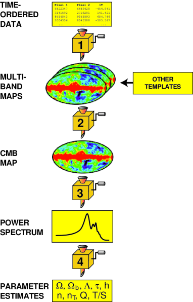
Comparing these observations with theoretical predictions to achieve this goal in practice is highly non-trivial, even aside from the experimental challenge of controlling systematic errors, and is often broken down into several steps, schematically illustrated in Figure 1:

1. Compress the time-ordered data set into sky maps at various frequencies, so as to minimize the effect of correlated detector noise, scan-synchronous offsets, and other non-sky signals (Wright 1996; Tegmark 1997a).

2. Compress the multi-frequency maps into a single CMB map so as to minimize the contribution of detector noise and foreground contamination (see Tegmark et al. 2000 and references therein).

3. Compress this CMB map into measurements of the angular power spectrum on various angular scales (Tegmark 1997b; Bond, Jaffe & Knox 1998), a step nicknamed “radical compression” by Bond et al.

4. Convert these power spectrum measurements into constraints on cosmological parameters.

This paper is focused on the last of these four steps, describing a method and applying it to all currently available data.

Since fast and accurate software is now available for computing how the theoretically predicted power spectrum depends on the cosmological parameters, this last step may at first appear rather trivial: just run a code such as CMBfast (Seljak & Zaldarriaga 1996) at a fine grid of points in parameter space and perform a $\chi^{2}$ fit of the corresponding theoretical power spectra to the observed data. The problem is that the currently most popular cosmological model has of order $N=10$ free parameters, making such an $N$-dimensional parameter grid rather huge and unwieldy. There are also additional challenges related to evaluating the likelihood function (Bond et al. 1998; Bartlett et al. 1999) that we will discuss in more detail below.

The first analyses based on COBE DMR used $N=2$ parameters, the scalar quadrupole normalization $A_{s}$ and tilt $n_{s}$ of the power spectrum (e.g., Smoot et al. 1992; Gorski et al. 1994; Bond 1995; Bunn & Sugiyama 1995; Tegmark & Bunn 1995). Since then, many dozens of papers have extended this to incorporate more data and parameters, with recent work including Bunn & White (1997); de Bernardis et al. (1997); Ratra et al. (1999); Hancock et al. (1998); Lesgourges et al. (1999); Bartlett et al. (1998); Webster et al. (1998); Lineweaver & Barbosa (1998ab); White (1998); Bond & Jaffe (1998); Gawiser & Silk (1998); Contaldi et al. (1999), Griffiths et al. 1999; Melchiorri et al. (1999); Rocha (1999).

In an important paper, Lineweaver (1998) made the leap up to $N=6$ parameters: $n_{s}$, $A_{s}$, the Hubble constant $h$ and the relative densities $\Omega_{\rm cdm}$, $\Omega_{\rm b}$ and $\Omega_{\Lambda}$ of CDM, baryons and vacuum energy, thereby setting a new standard. Tegmark (1999, hereafter T99) pushed on to $N=8$ by adding the reionization optical depth $\tau$ and the gravity wave amplitude $A_{t}$. Efstathiou et al. (1999), Efstathiou (1999), Bahcall et al. (1999), Dodelson & Knox (2000) and Melchiorri et al. (2000) performed analyses with different techniques, better data and around 6 parameters, all finding interesting joint constraints on $\Omega_{\Lambda}$ and the matter density. Despite this progress, however, a number of issues still need to be improved to do justice to the ever-improving data.

Perhaps the most glaring problem is that no closed models (White & Scott 1996) have ever been computed exactly in these analyses, except for that of Melchiorri et al. (2000), since the CMBfast software was limited to flat and open models. We remedy this in the present paper by using version 3.2 of CMBfast (Zaldarriaga & Seljak 1999), which is generalized to closed models. A new code by Challinor et al. (2000), based on CMBfast, also does closed models, agreeing well with CMBfast.

Another problem with all previous analyses is that they assumed the massive neutrino density $\Omega_{\nu}$ to be zero, although there is strong evidence from both the atmospheric and solar neutrino anomalies that $\Omega_{\nu}>0$. Since these particle physics constraints are only sensitive to the differences between the (squared) masses of the various neutrinos, they do not imply that neutrinos are astrophysically uninteresting. Indeed, because the CMB and matter power spectra can place some of the most stringent upper limits on neutrino masses (Hu et al. 1998), it would be a real pity to omit this aspect of the analysis. Just as increasing $\Omega_{\rm cdm}$ suppresses the acoustic peaks, increasing $\Omega_{\nu}$ suppresses does so by a comparable amount. Indeed, these two parameters become nearly degenerate for large $\Omega_{\nu}$, corresponding to neutrinos massive enough to be fairly nonrelativistic at the relevant redshifts, so the inclusion of neutrinos will, among other things, weaken the lower limit on $\Omega_{\rm cdm}$.

Another weakness of the T99 analysis was that it assumed that the relative amplitude $r\equiv A_{t}/A_{s}$ of gravity waves was linked to the tensor spectral index by the inflationary consistency relation $r=-7n_{t}$ (Liddle & Lyth 1992), although one of the most exciting applications of CMB data will be to test this relation. We will remedy both of these problems by extending our parameter space to $N=10$ dimensions, including both $\Omega_{\nu}$ and $n_{t}$ as free parameters.

Finally, as we will discuss at length below, there are a number of areas where accuracy has been unsatisfactory and can be substantially improved.

The rest of this paper is organized as follows. We describe our method in Section 2, apply it to the available data in Section 3 and summarize our conclusions in Section 4. Some technical details regarding marginalization are derived in the Appendix.

2. METHOD

Figure 2.— The band power measurements used.

2.1. The problem

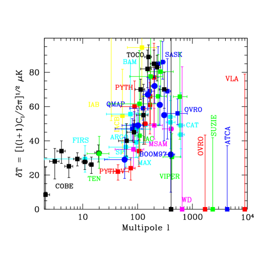
Our data consists of the $n=65$ band power measurements $\delta T^{2}_{i}$ listed in Table 1 and shown in Figure 2, $i=1,...,n$. The band power measurement $d_{i}\equiv\delta T^{2}_{i}$ probes a weighted average of $\delta T_{\l}^{2}\equiv\l(\l+1)C_{\l}/2\pi$,

$$\langle d_{i}\rangle=\langle\delta T^{2}_{i}\rangle=\sum_{\l}{1\over\l}W^{i}_{\l}\delta T_{\l}^{2},$$ (1)

where $W^{i}_{\l}$ is the band-power window function (distinct from the variance window function; see Knox 1999). These known weights $W^{i}_{\l}$ reflect which angular scales the measurement is sensitive to.

The power spectrum in turn depends on our vector of cosmological parameters ${\bf p}$ in a complicated fashion $C_{\l}({\bf p})$ that we use CMBfast to compute. The scatter in the relation between $d_{i}$ and $\langle d_{i}\rangle$ due to detector noise and sample variance is described by a likelihood function $\L_{i}(d_{i};C_{\l}({\bf p}))$, the probability distribution for $d_{i}$ given ${\bf p}$. If the errors in the different data points were all independent, then the combined likelihood of observing the set of all data given ${\bf p}$ would be simply

$$\L({\rm data};{\bf p})=\prod_{i=1}^{n}\L_{i}(d_{i};C_{\l}({\bf p})).$$ (2)

This is complicated by the fact that some measurements are correlated, as will be discussed in Section 2.7.

Our problem is to evaluate this likelihood function in the 10-dimensional parameter space that ${\bf p}$ inhabits. To obtain Bayesian constraints on individual parameters or joint constraints on interesting pairs (such as $\Omega_{\rm m}$ and $\Omega_{\Lambda}$), we then marginalize over the remaining parameters with appropriate priors.

2.2. Breaking it into four sub-problems

If we had infinite computing resources, the solution would be straightforward: compute the theoretical CMB power spectrum $C_{\l}({\bf p})$ with the CMBfast software (Seljak & Zaldarriaga 1996) and the corresponding likelihood at a fine grid of points in the $N$-dimensional parameter space. In practice, this is inconvenient. With $M$ grid points in each dimension, $M^{N}$ power spectra must be computed. Even if we take $M$ as low as 10, the amount of work thus grows by an order of magnitude for each additional parameter. With 1 minute per power spectrum calculation, $N=10$ would translate to over $10^{4}$ years of CPU time.

Fortunately, the underlying physics (see e.g. Hu et al. 1997 for a review) allows several numerical simplifications to be made. We will adopt the approximation scheme used in T99 with additional improvements as described below. Our method conveniently separates into four separate steps.

• Step 1: Run CMBfast many times for three particular subsets of the parameter grid. The results are three large files: one with tensor power spectra, one with scalar power spectra for $\ell\mathrel{\hbox to0.0pt{\lower 3.0pt\hbox{$\mathchar 536\relax$}\hss}\raise 2.0pt\hbox{$\mathchar 316\relax$}}100$ and one with scalar power spectra for $\ell\mathrel{\hbox to0.0pt{\lower 3.0pt\hbox{$\mathchar 536\relax$}\hss}\raise 2.0pt\hbox{$\mathchar 318\relax$}}100$.

• Step 2: Interpolate these spectra onto larger subsets of the parameter grid. The results are two huge files with 7-dimensional model grids, one for scalars and one for tensors. These two files allow any power spectrum in the full 10-dimensional model grid to be computed almost instantaneously.

• Step 3: Compute and save the likelihood $\L$ for each model.

• Step 4: Perform 10-dimensional interpolation and marginalize to obtain constraints on individual parameters, constraints in the $(\Omega_{\rm m},\Omega_{\Lambda})$-plane, etc.

Below we will describe each of these four steps in turn. Before doing this, however, it is interesting to contrast this “huge grid” approach with an alternative strategy. Dodelson & Knox (2000) and Melchiorri et al. (2000) performed their analyses without computing and storing such a grid. Instead, they found the maximum-likelihood parameter vector ${\bf p}$ by a direct numerical maximum search, computing power spectra with CMBfast on the fly as needed. Similarly, constraints in say the $(\Omega_{\rm m},\Omega_{\Lambda})$-plane were obtained by performing a numerical maximum search over the remaining parameters for each $(\Omega_{\rm m},\Omega_{\Lambda})$ grid point. One drawback of this approach is that everything needs to be repeated from scratch if the data set is changed, whereas steps 1 and 2 in our method are independent of the data set and need only be done once and for all. The same drawback applies to exploring different priors. There is also no guarantee that CMBfast gets run fewer times with this direct search approach, as a numerical search in the high-dimensional space tends to require large numbers of likelihood evaluations (Dodelson 1999, private communication; see also Hannestad 1999).

2.3. Parameter space

We choose our 10-dimensional parameter vector to be

$${\bf p}\equiv(\tau,\Omega_{\rm k},\Omega_{\Lambda},\omega_{\rm cdm},\omega_{\rm b},\omega_{\nu},n_{s},n_{t},A_{s},A_{t}),$$ (3)

where the physical densities $\omega_{i}\equiv h^{2}\Omega_{i}$, $i=$cdm, b, $\nu$. The advantage of this parameterization (see Bond et al. 1997) will become clear in §2.5. $\Omega_{\rm k}$ is the spatial curvature, so in terms of these parameters,

$$h=\sqrt{\omega_{\rm cdm}+\omega_{\rm b}+\omega_{\nu}\over 1-\Omega_{\rm k}-\Omega_{\Lambda}}.$$ (4)

This parameter space is identical to that used in T99 except that we have added $\omega_{\nu}$ and replaced $h$ by $\Omega_{\Lambda}$ as a free parameter.

We wish to probe a large enough region of parameter space to cover even quite unconventional models. This way, constraints from non-CMB observations can be optionally included by explicitly multiplying $\L({\bf p})$ by a Bayesian prior after Step 3 rather than being hard-wired in from the outset. To avoid prohibitively large $M$, we use a roughly logarithmic grid spacing for $\omega_{\rm m}$, $\omega_{\rm b}$ and $\omega_{\nu}$, a linear grid spacing for $\Omega_{\rm k}$ and $\Omega_{\Lambda}$, a hybrid for $\tau$, $\omega_{\nu}$, $n_{s}$ and $n_{t}$, and (as described below) no grid at all for $A_{s}$ and $A_{t}$. We let the parameters take on the following values:

• $\tau=0,0.05,0.1,0.2,0.3,0.5,0.8$

• $\Omega_{\Lambda}=-1.0,-0.8,-0.6,-0.4,....,1.0$

• $\Omega_{\rm k}$ such that $\Omega_{\rm m}\equiv 1-\Omega_{\rm k}-\Omega_{\Lambda}=0.2,0.4,...,2.0$

• $\omega_{\rm cdm}=0.02,0.03,0.05,0.08,0.13,0.2,0.3,0.5,0.8$

• $\omega_{\rm b}=0.003,0.005,0.008,0.013,0.02,0.03,0.05,0.08,0.13$

• $\omega_{\nu}=0,0.02,0.05,0.08,0.13,0.2,0.3,0.5,0.8$

• $n_{s}=0.50,0.70,0.90,1.00,1.10,1.20,1.30,1.50,1.70$

• $n_{t}=-1.00,-0.70,-0.40,-0.20,-0.10,0$

• $A_{s}$ is not discretized

• $A_{t}$ is not discretized

Note that the extent of the $\Omega_{\rm k}$-grid depends on $\Omega_{\Lambda}$, giving a total of $10\times 11=110$ points in the $(\Omega_{\rm m},\Omega_{\Lambda})$-plane. Our discrete grid thus contains $7\times 110\times 9\times 9\times 9\times 9\times 6=30,311,820$ models. As will become clear from our discussion below, the main limitation on this grid size is the disk space used in Step 2 rather than the CPU time used in Step 1, so it will probably be desirable to further refine it as CMB data gets better.

2.4. Separating scalars and tensors

If we were to run CMBfast in the standard way, computing scalar and tensor fluctuations simultaneously, we would have to explore a 9-dimensional model grid since only $A_{s}$ drops out as an overall normalization factor. Instead, we compute the scalar fluctuations $C_{\ell}^{scalar}$ and the tensor fluctuations $C_{\ell}^{tensor}$ separately, normalize them to both have a quadrupole of unity, and compute the combined power spectrum as

$$C_{\ell}=A_{s}C_{\ell}^{scalar}+A_{t}C_{\ell}^{tensor}.$$ (5)

We therefore only need to compute two 7-dimensional grids with CMBfast, one over $(\tau,\Omega_{\rm k},\Omega_{\Lambda},\omega_{\rm cdm},\omega_{\rm b},\omega_{\nu},n_{s})$ and the other over $(\tau,\Omega_{\rm k},\Omega_{\Lambda},\omega_{\rm cdm},\omega_{\rm b},\omega_{\nu},n_{t})$. The other advantage of calculating scalars and tensors separately is that tensors only need to be calculated up to an $l$ of 400, which saves additional time.

Allowing 1 minute per model, the scalar grid alone would still take about 10 years of CPU time. Most models take substantially longer to run, since reionization, curvature and neutrinos slow CMBfast down. It is therefore useful to take advantage of the underlying physics to make further simplifications.

2.5. Separating small and large scales

The tensor power spectrum depends only weakly on $\omega_{\rm cdm}$, $\omega_{\rm b}$ and $\omega_{\nu}$. We therefore compute the tensor power spectrum with the fine grid restricted to $(\tau,\Omega_{\rm k},\Omega_{\Lambda},n_{t})$, using only ultra-course three-point grids for $\omega_{\rm cdm}$, $\omega_{\rm b}$ and $\omega_{\nu}$. We then fill in the rest of the $(\omega_{\rm cdm},\omega_{\rm b},\omega_{\nu})$-values using cubic spline interpolation.

The scalar power spectrum $C_{\ell}$ for $\l\ll 100/\Omega_{\rm m}^{1/2}$ corresponds to fluctuations on scales outside the horizon at recombination. This makes it almost independent of the causal microphysics that create the familiar acoustic peaks, i.e., independent of $\omega_{\rm m}$, $\omega_{\nu}$ and $\omega_{\rm b}$. We therefore compute the scalar power spectrum on large scales with the fine grid restricted to $(\tau,\Omega_{\rm k},\Omega_{\Lambda},n_{s})$, using only ultra-course three-point grids for $\omega_{\rm cdm}$, $\omega_{\rm b}$ and $\omega_{\nu}$ to to pick up weak residual effects aliased down from larger $\l$. We then fill in the rest of the $(\omega_{\rm cdm},\omega_{\rm b},\omega_{\nu})$-values using cubic spline interpolation.

For the remaining (high $\l$) part of the power spectrum, more radical simplifications can be made. First of all, the effect of reionization is mainly an overall suppression of $C_{\ell}$ by a constant factor $e^{-2\tau}$ on these small scales. Second, the effect of changing both $\Omega_{\rm k}$ and $\Omega_{\Lambda}$ is merely to shift the power spectrum sideways. This is because the acoustic oscillations at $z\mathrel{\hbox to0.0pt{\lower 3.0pt\hbox{$\mathchar 536\relax$}\hss}\raise 2.0pt\hbox{$\mathchar 318\relax$}}1000$ (at which time $\Omega_{\rm k}\approx\Omega_{\Lambda}\approx 0$ regardless of their present value) depend only on $\omega_{\rm m}$, $\omega_{\rm b}$ and $\omega_{\nu}$, and the geometric projection of these fixed length scales onto angular scales $\theta$ in the sky obeys $\theta\propto 1/d_{\rm lss}$, where $d_{\rm lss}$ is the angular diameter distance to the last scattering surface. In T99 and Efstathiou et al. (1999), $d_{\rm lss}$ was estimated analytically by integrating out to the redshift of last scattering given by the fit of Hu & Sugiyama (1996). Since CMBfast automatically computes this quantity anyway, we eliminate this approximation by simply using this numerical value.

$\Omega_{\rm m}$ and $\Omega_{\Lambda}$ also modify the late integrated Sachs-Wolfe effect, but this is important only for $\l\mathrel{\hbox to0.0pt{\lower 3.0pt\hbox{$\mathchar 536\relax$}\hss}\raise 2.0pt\hbox{$\mathchar 316\relax$}}30$ (Eisenstein et al. 1999). The only other effect is a small correction due to gravitational lensing (Metcalf & Silk 1997; Stompor & Efstathiou 1999), which we ignore here because of the large error bars on current small-scale data. To map the model ${\bf p}^{*}$ into the model ${\bf p}$ with all parameters except $\tau$, $\Omega_{\rm k}$ and $\Omega_{\Lambda}$ unchanged, we thus multiply its high $\l$ power spectrum by $e^{2(\tau^{*}-\tau)}$ and shift it to the right by an $\l$-factor of $d_{\rm lss}/d_{\rm lss}^{*}$.

We therefore adopt the following procedure for the first two steps. In Step 1, we compute

• scalar power spectra out to $\l=5000$ for the subgrid with $\tau=\Omega_{\rm k}=\Omega_{\Lambda}=0$ (merely 6,561 models),

• scalar power spectra out to $\l=400$ with the subgrid restricted to $\tau=0,0.1,0.8$, $\omega_{\rm m}=0.02,0.2,0.8$, $\omega_{\rm b}=0.003,0.02,0.13$, $\omega_{\nu}=0,0.2,0.8$ (80,190 models), and

• tensor power spectra with the matter densities restricted to this same subgrid (80,190 models).

In Step 2, we use cubic spline interpolation separately for each $\l$ to extend the tensor models and the low-$\ell$ scalar models to the full parameter grid. To account for the effects of $\tau$, $\Omega_{\rm k}$ and $\Omega_{\Lambda}$, we then shift the high-$\ell$ scalar models vertically and horizontally as described above and splice them together with the corresponding low-$\l$ models at a cutoff value $\l^{*}$. For a given model, we choose $\l^{*}$ to be 100 multiplied by the horizontal shifting factor. In other words, the high-$\ell$ model always gets spliced at the location that corresponded to $\l=100$ before shifting it sideways, so open models get spliced at higher $\l$ and closed at lower. When computing the low-$\ell$ models in Step 1, we therefore adjust the accuracy flag “ketamax” in CMBfast to be 400 times this same shifting factor.

The public releases of CMBfast normalize the power spectra $C_{\l}$ to COBE automatically. This normalization scheme is not appropriate for our merging technique, since we need a convention independent of the cosmological parameters so that when we combine the high and low grids, the relative normalization of the models is correct. To achieve this, we removed the COBE normalization from CMBfast and normalized the power spectrum in both the flat and non-flat codes to agree on scales much smaller than the curvature scale.

For the reader interested in implementing this scheme, it is worth noting that almost all the time in Step 1 is spent on the low scalar grid. For this grid, substantial time is saved by only computing the power spectrum for the low $\l$-values where it is needed. Note that the loop over tilts ($n_{s}$ or $n_{t}$) is essentially free, since CMBfast can compute multiple tilts simultaneously. The only reason we have used so few tilt values is because of disk space considerations in Steps 2 through 4. Including various test runs, we filled up more than half of a 200 GB disk array.

2.6. Testing step 2

To test the accuracy of the resulting scalar and tensor model grids produced in Step 2, we drew a random sample of $\sim 10^{3}$ of the models and recomputed them from scratch with CMBfast. For most models, we found our results to be accurate to a within a few percent. The remainder generally had very early reionization (high $\tau$ and low $h\Omega_{\rm b}$), which causes a broad bump of regenerated power from motions on the new last scattering surface. Since our approximation simply suppresses the small scale power by $e^{-2\tau}$, it therefore underpredicts the power on the angular scale corresponding to the horizon size at reionization. In addition, the interpolation performed poorly at the lowest $\l$ for some quite crazy models, which could be remedied by running CMBfast on a finer grid.

As data quality improves further, it will probably be worthwhile to simply include $\tau$ explicitly in the high-$\l$ grid. In this case, the remaining errors introduced by our approximation scheme can of course be continuously reduced to zero by refining the $(\omega_{\rm cdm},\omega_{\rm b},\omega_{\nu})$-grid for low $\l$ and shifting the splicing point upwards from $\l\sim 100$.

2.7. Step 3: computing likelihoods

We use the CMB data and window functions listed in Table 1 and shown in Figure 2. This is taken from the compilation of Lineweaver (1998) with the addition of the new results from QMAP (Devlin et al. 1998; Herbig et al. 1998; de Oliveira-Costa et al. 1998), MSAM (Wilson et al. 1999), Toco (Torbet et al. 1999; Miller et al. 1999), Python V (Coble 1999), Viper (Peterson et al. 2000) and Boomerang (Mauskopf et al. 1999). For an up-to-date annotated compilation of all current data, see Gawiser & Silk (2000). For the COBE data, we use the exact window function from Tegmark (1997b). In all other cases, we approximate the window functions by a Gaussian of FWHM=$\l_{\rm high}-\l_{\rm low}$ from Table 1. This approximation does not appear to have much of an effect on the results: we repeated the analysis with the much more extreme approximation where the windows are delta functions at $(\l_{\rm low}+\l_{\rm high})/2$ and obtained essentally unchanged results. Knox & Page (2000) compared full window functions with delta functions and came to the same conclusion.

As discussed in great detail by Bond, Jaffe & Knox (1998) and also by Bartlett et al. (1999), an accurate calculation of the likelihood function $\L({\rm data}|{\bf p})$ is nontrivial. If the band-power measurement $d_{i}$ is a quadratic function of the sky temperatures measured by the experiment in question, then $\L_{i}(d_{i};C_{\l}({\bf p}))$ is a generalized $\chi^{2}$ distribution when viewed as a function of $d_{i}$ (Wandelt et al. 1998), but sufficient details to compute this function exactly are rarely published when band power measurements are released. Useful approximations have therefore been derived that require only the asymmetry between upper and lower error bars as input (Bond, Jaffe & Knox (1998), Bartlett et al. (1999). The former approximation is implemented by a nice publicly available package called RADPACK, maintained by Lloyd Knox at http://flight.uchicago.edu/knox/radpack.html, which was used in the analyses of Dodelson & Knox (2000) and Melchiorri et al. (2000). In this paper, we will stick with the cruder Gaussian approximation

$$\L({\bf d};C_{\l}({\bf p}))\approx e^{-{1\over 2}({\bf d}-\langle{\bf d}\rangle)^{t}{\bf C}^{-1}({\bf d}-\langle{\bf d}\rangle)},$$ (6)

where ${\bf d}$ is the vector of measurements $d_{1},d_{2},...d_{n}$ and ${\bf C}$ is the associated $n\times n$ covariance matrix of measurement errors. This means that the full likelihood function $\L=e^{-\chi^{2}/2}$, where $\chi^{2}$ is simply the chi-squared goodness of fit of the model to the data.

We have chosen to keep things this simple because we are currently unable to eliminate a third major source of inaccuracy: many of the recent multi-band measurements released (which dominate the constraining power) have non-negligible correlations between their different bands, but these correlations have not yet been published by the experimental teams. An alternative approach would be to convert these data sets to uncorrelated measurements, as was done with the 8 COBE points we use. In the interim, an alternative is to simply use only those experiments which either have very small correlations, or significant correlations which are publically available, as was done in Dodelson & Knox (2000) and Knox & Page (2000).

We model ${\bf C}$ as a sum of three terms, ${\bf C}={\bf C}^{\rm(meas)}+{\bf C}^{\rm(scal)}+{\bf C}^{\rm(ical)}$, corresponding to measurement errors, source calibration errors and instrument calibration errors, respectively. ${\bf C}^{\rm(meas)}$ reflects the part of the errors which are uncorrelated between the different experiments and is due to detector noise and sample variance. We approximate it by

$${\bf C}^{\rm(meas)}_{ij}\equiv\delta_{ij}\sigma_{i}^{2},$$ (7)

where $\sigma_{i}$ is defined as the average of the upper and lower error bars quoted for $d_{i}\equiv\delta T^{2}$ (not for $\delta T$) in Table 1.

The last two terms reflect the correlations between measurements due to calibration errors. ${\bf C}^{\rm(ical)}$ is the part specific to a single multi-band experiment and ${\bf C}^{\rm(scal)}$ is the part that is correlated with other experiments that are calibrated off of the same (slightly uncertain) source. Both QMAP and Saskatoon calibrate off of Cass A, and we assume that a 8.7% error due to the flux uncertainty of this object is common to these experiments. MAT, MSAM and Boomerang all calibrate off of Jupiter. To be conservative, we assume that the full 5% calibration uncertainty from Jupiter’s antenna temperature is shared by these experiment. The true correlation should be lower, since the three experiments observed Jupiter at different frequencies. The remaining multi-band experiments do not have any such inter-experiment correlations: COBE/DMR calibrated off of the dipole, Viper off of the moon and Python V off of internal loads. This contribution to the noise matrix is therefore

$${\bf C}^{\rm(scal)}_{ij}\equiv(2s_{ij})^{2}d_{i}d_{j},$$ (8)

where

$$s_{ij}=\cases{8.7\%&if $i$ and $j$ refer to QMAP or Saskatoon,\cr 5\%&if $i$ and $j$ refer to MAT, MSAM or Boom,\cr 0&otherwise.\cr}$$ (9)

The factor of 2 in equation (8) stems from the fact that the percentage error on $\delta T_{i}^{2}$ is roughly twice that for $\delta T_{i}$ as long as it is small. Similarly, the remaining term is

$${\bf C}^{\rm(ical)}_{ij}\equiv(2r_{ij})^{2}d_{i}d_{j},$$ (10)

where $r_{ij}=0$ if $i$ and $j$ refer to different experiments. If band powers $i$ and $j$ are from the same experiment, then $r_{ij}$ is the quoted quoted calibration error with the source contribution $s_{ij}$ subtracted off in quadrature. We use $r=$0.063 for Saskatoon, 7.9% for QMAP, 14% for Python V, 8% for Viper, 8.7% for Toco 97, 6.2% for Toco 98, 0 for MSAM and 6.4% for Boomerang.

There is certainly ample room for improvement of in this 3rd step. To put all these statistical issues in perspective, however, the authors feels that an even more pressing challenge will be to test the data sets for systematic errors, e.g., by comparing them pairwise where they overlap in sky coverage and angular resolution (Knox et al. 1998; Tegmark 1999a).

2.8. Step 4: Marginalizing

For a Bayesian analysis, the 10-dimensional likelihood should be multiplied by a prior probability distribution reflecting all non-CMB information, then rescaled so that it integrates to unity and can be interpreted as a probability distribution. To obtain constraints on some subset of the parameters ($\Omega_{\rm k}$ and $\Omega_{\Lambda}$, say), one would then marginalize over all other parameters by integrating over them. Such a direct integration was performed by Efstathiou et al. (1999) where the parameter space had fewer dimensions. Since such integration is quite time-consuming in a high-dimensional space, most other multi-parameter analyses published have adopted the alternative approach of maximizing rather than integrating over the unwanted parameters. For instance, the reduced likelihood function for $\tau$ is obtained by looping over a grid of $\tau$-values and choosing the remaining parameters so that they maximize the likelihood in each case. These two approaches are equivalent if the full likelihood function is a multivariate Gaussian, as shown in Appendix A. If Gaussianity is a poor approximation, the maximization approach can tend to underestimate the error bars (Efstathiou et al. 1999). The Gaussianity approximation is indeed a poor one at the moment, especially for the case with no priors, but it should gradually improve as future data and non-CMB priors reduce the size of the allowed parameter region.

In the published grid-based implementations of the maximization method (e.g., Lineweaver 1998; T99), the minimization was performed by simply looking at the likelihoods in the pre-computed model grid and picking the largest one. Since the true maximum does generally not reside exactly at a grid point, this method always underestimates the true maximum. Unfortunately, the magnitude of this underestimation will vary in a rather random way, depending on how close to the constrained maximum happens to be to the nearest grid point. This effect can cause jagged-looking and somewhat misleading results, as shown in Figure 3. Note that even an error as small as 0.5 in $\chi^{2}$ changes the likelihood by more than 20%. Some of the jaggedness/ringing seen in the plots in, e.g., Lineweaver (1998) and T99 is likely to be due to this effect. In contrast, the ringing seen in many of the $(\Omega_{\rm m},\Omega_{\Lambda})$ exclusion plots further on in this paper is a purely cosmetic problem, due to instability in the IDL interpolation routine used to generate the contour plots.

Figure 3.— Marginalization method comparison. $\chi^{2}$ is plotted as a function of $\Omega_{\Lambda}$ when maximizing over all other parameters with no priors. The squares show the result of using multidimensional spline interpolation when maximizing and the crosses show the result of simply picking the smallest $\chi^{2}$-value in the model grid. Note that a seemingly small error of unity in $\chi^{2}$ changes the likelihood by a factor of 1.6.

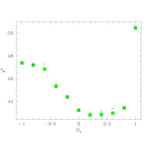
The problem at hand is to find the maximum of some hypersurface in a high-dimensional space. It is easy to see that if we approximate the surface by multilinear interpolation between the grid points where we know its height, we will recover this unsatisfactory method, since the interpolated surface can only have maxima at grid points. We have chosen to use cubic spline interpolation instead. As seen in Figure 3, this works substantially better and eliminates the random jaggedness of the simpler method.

For the reader interested in implementing this method, we give some additional practical details below. Other readers may wish to skip directly to the next subsection.

We perform the cubic spline interpolation and subsequent maximization one dimension at a time. Just as for multilinear interpolation, the result of this procedure is independent of the order in which we interpolate over the different parameters. We start by maximizing over the scalar and tensor normalizations, which is readily done analytically since $\chi^{2}$ depends quadratically on $A_{s}$ and $A_{t}$. We save the remaining 8-dimensional grid in a huge file together with the optimal values of $A_{s}$ and $A_{t}$ and the corresponding $\chi^{2}$ value. To marginalize over any given parameter $p_{i}$, we first sort this file so that this parameter varies fastest. In each block where the remaining parameters are fixed, we then spline over this parameter and find the maximum $p_{i}^{*}$ analytically from the spline coefficients. Since it is interesting to keep track of the physical parameters of the best fit models, we save not only the $\chi^{2}$-value but also the other parameter values spline interpolated to the point where $p_{i}=p_{i}^{*}$, replacing the entire block of models in the file by this interpolated one.

We found that when $\chi^{2}$ varies rapidly, a standard cubic spline occasionally causes unwanted oscillations. Such a rapid rise in $\chi^{2}$ occurs only in the extreme parts of the parameter grid that we do not care about (since they are completely ruled out), yet the resulting ringing easily propagates to the region that we are interested in near the minimum. We therefore adopted a scheme where we through away irrelevant distant points before splining if they were too extreme. Specifically, before performing a 1-dimensional cubic spline, we first located the lowest grid point. We then included all points to the left of it until we reached one whose $\chi^{2}$ was higher by 10 or more. Points to the right were included analogously. We found this simple scheme to work quite well in practice. Indeed, the slight wiggliness of the contour plots shown in the next section is caused mainly by the plotting software itself (the 2D interpolation routine of IDL), not by our marginalization from 10 to 2 dimensions.

3. RESULTS

3.1. Basic results

To avoid having our constraints severely diluted by “silly” models, we include two prior pieces of information when presenting our basic results. We assume that the Hubble parameter $h=0.65\pm 0.07$ at $1-\sigma$ (see Freedman 1999 for a recent review of $h$-measurements) and that the baryon density $\omega_{\rm b}=h^{2}\Omega_{\rm b}\approx 0.02$ (Burles et al. 1999 report $\omega_{\rm b}=0.019\pm 0.0024$, and we approximate the $\omega_{\rm b}$ error bars by zero since they are much smaller than our $\omega_{\rm b}$ grid spacing). This value of $\omega_{\rm b}$ is roughly consistent with that measured by Wadsley et al. (1999) using the Helium Lyman-Alpha Forest. We assume that the error distribution for $h$ is Gaussian.

Figure 4.— The best fit model is shown for the case of no prior (solid red/dark grey) and with the priors $h=0.65\pm 0.07$, $h^{2}\Omega_{\rm b}=0.02$ and $\tau=r=0$ (solid green/light grey). The dotted lines show the decomposition of the former curve into scalar and tensor fluctuations. The model parameters are listed in Table 2. Although all 65 measurements were used in the fits, they have been averaged into 14 bands in this plot to avoid cluttering. The band powers whose central $\l$-value fell into any given band were average with minimum-variance weighting, and their corresponding window functions were averaged as well. This binning was used only in this plot, not in our analysis.

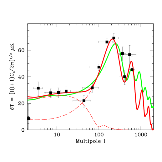
Table 2 – Maximum-likelihood values and 95% confidence limits 10 free parameters $h$ & $\omega_{\rm b}$ prior Quantity Min Best Max Min Best Max $\tau$ 0.0 0.0 $-$ 0.0 0.0 $-$ $\Omega_{\rm k}$ $-$1.74 $-$1.03 0.49 $-$0.24 .09 0.38 $\Omega_{\Lambda}$ $-$ .16 $-$ $-$0.19 .67 0.89 $h^{2}\Omega_{\rm cdm}$ 0.0 .53 $-$ 0.0 .036 0.30 $h^{2}\Omega_{\rm b}$ .11 .13 $-$ .02 .02 .02 $h^{2}\Omega_{\nu}$ 0.0 .012 $-$ 0.0 .051 .29 $n_{s}$ .55 1.69 $-$ 0.80 1.05 1.53 $n_{t}$ $-$ 0.00 $-$ $-$ 0.03 $-$

The parameters of the best fit model are listed in Table 2 both with and without these priors. The corresponding no-prior power spectrum is shown in Figure 4 together with the “vanilla” version with the above-mentioned priors and $\tau=r=0$. As can be seen, the fitting procedure uses the additional freedom to match features in the data in quite amusing ways. Since the data dip at $\l\sim 50$ and rise very sharply thereafter, a feature that simpler models cannot match, the minimization procedure finds the best fit model to have a dramatic blue-tilt ($n_{s}\sim 1.7$) and almost the entire COBE signal due to gravity waves. Although this particular model is ruled out by other constraints — for instance, primordial black hole abundance (Green et al. 1997) and spectral distortions (Hu et al. 1994) give upper bounds $n_{s}\mathrel{\hbox to0.0pt{\lower 3.0pt\hbox{$\mathchar 536\relax$}\hss}\raise 2.0pt\hbox{$\mathchar 316\relax$}}1.3$) — it illustrates the importance of fitting for all 10 parameters jointly. Indeed, it is the inclusion of gravity waves in our models that makes the constraints on $n_{s}$ so weak.

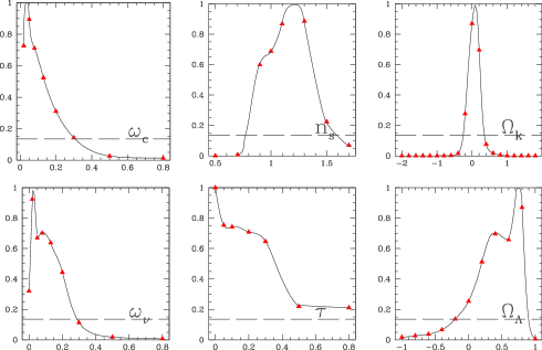
The 1-dimensional likelihood functions for six of the best constrained parameters are shown in Figure 5, marginalized over the other 9 parameters. Although none of these parameters are very tightly constrained, it is encouraging that CMB observations are already sufficiently powerful to place upper and lower limits on $\Omega_{\rm m}$, $\Omega_{\Lambda}$ and $n_{s}$ at the $2-\sigma$ level. Because $\omega_{\rm cdm}$ and $\omega_{\nu}$ are by definition non-negative, these density parameters are also bounded from both sides. On the other hand, better data will be required to place interesting constraints on $\tau$, since this parameter is almost degenerate with the overall normalization (see, e.g., Eisenstein et al. 1999). The best constrained parameter so far is seen to be the spatial curvature $\Omega_{\rm k}$, with $-0.24<\Omega_{\rm k}<0.38$ at 95% confidence. For comparison, using Figure 2 in Dodelson & Knox (2000) to read off the point where the likelihood drops to $e^{-2^{2}/2}\approx 0.14$ gives the 95% upper limit $\Omega_{\rm k}<0.38$. Although the exact numerical agreement is likely to be coincidental (since we use more data, etc), this is nonethetheless very reassuring evidence that the basic result is robust.

Figure 5.— The marginalized likelihood is shown for six individual parameters using all 65 band power measurements and priors only from nucleosynthesis ($h^{2}\Omega_{\rm b}=0.02$) and the Hubble parameter ($h=0.65\pm 0.07$). The $2\sigma$ limits (see Table 2) are roughly where the curves cross the horizontal lines.

Because of the well-known angular diameter distance degeneracy, where increasing $\Omega_{\rm k}$ shifts the acoustic peaks to the right and increasing $\Omega_{\Lambda}$ can shift them back to the left, we also plot our constraints marginalized onto the 2-dimensional $(\Omega_{\rm m},\Omega_{\Lambda})$-plane. Figure 6 shows the results using all the data, and Figures 7– 9 shown the constraints from various subsets that will be described below. In all cases, the shaded regions show what is ruled out at 95% confidence ($2-\sigma$). For our 2-dimensional parameter space, this corresponds to $\Delta\chi^{2}=6.18$ (not 4), as in Press et al. (1992) §15.6.

We show four nested contours. The least constraining one is when all 10 parameters are treated as unknown. The second includes our Hubble parameter prior $h=0.65\pm 0.07$. The third (what we call our “basic result”) adds the nucleosynthesis constraint $\omega_{\rm b}\approx 0.02$ and the fourth imposes $r=\tau=0$. Although the first two priors are observationally well-motivated, the last one is completely ad hoc, and has only been included to illustrate the importance of including reionization and gravity waves in analyses of this kind.

When removing a prior constraint ($\omega_{\rm b}=0.02$) from our basic result, we reduce all $\chi^{2}$-values by unity before plotting the corresponding contour, to account for the added degree of freedom. Similarly, we subtract 2 when dropping both constraints and add 2 when imposing $\tau=r=0$.

Figure 6.— The regions in the $(\Omega_{\rm m},\Omega_{\Lambda})$-plane that are ruled out at $2\sigma$ using all the data are shown using no priors (red/dark grey), the prior $h=0.65\pm 0.07$ (orange red/grey), the additional nucleosynthesis constraint $h^{2}\Omega_{\rm b}=0.02$ (orange/light grey) and the additional constraints $r=\tau=0$ (yellow/very light grey).

Figure 7.— Same as previous figure, but using only the COBE and the “East Coast” data sets (Saskatoon, QMAP and Toco).

Figure 8.— Same as Figure 6, but using only COBE and “Snake” data sets (Python V and Viper).

Figure 9.— Same as Figure 6, but using only COBE and Boomerang data sets. The yellow/light grey contour corresponds to the result of Melchiorri et al (2000) if we impose $\omega_{\nu}=0$.

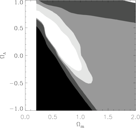
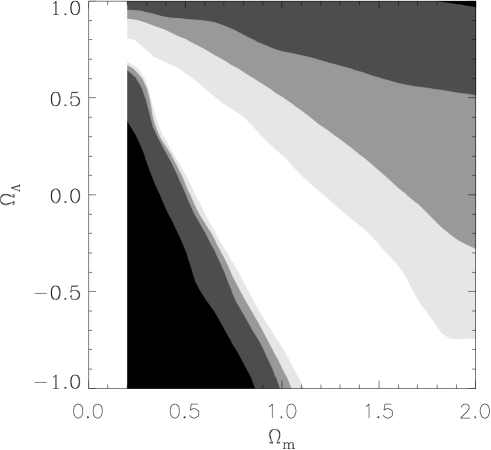
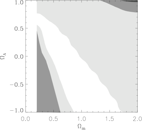
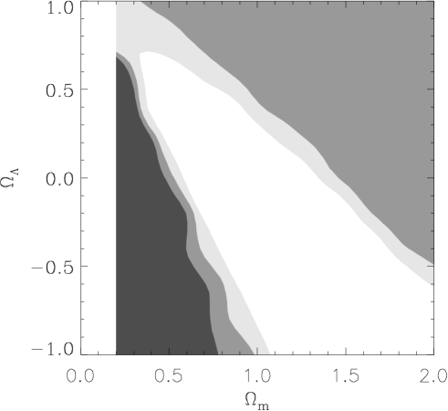
Figure 6 shows that the CMB data alone is able to rule out very open ($\Omega_{\rm m}\mathrel{\hbox to0.0pt{\lower 3.0pt\hbox{$\mathchar 536\relax$}\hss}\raise 2.0pt\hbox{$\mathchar 316\relax$}}0.4$) models with $\Omega_{\Lambda}=0$. Adding the $h$-constraint tightened the limits somewhat, mainly on very closed models. A more important prior at at this stage is that from nucleosynthesis, which helps eliminate most of the remaining closed models and places the first lower limit on $\Omega_{\Lambda}$. This makes the allowed region in the $(\Omega_{\rm m},\Omega_{\Lambda})$-plane bounded, which is important: otherwise all other constraints, which are marginalized over $\Omega_{\Lambda}$, would depend sensitively on the poorly motivated prior $\Omega_{\Lambda}\geq-1$ that was hard-wired into our parameter grid.

Adding the additional prior $\tau=r=0$, which we recommend against for the reasons described in the introduction, is seen to rule out about half of the remaining models. The exclusion of these parameters is seen to predominantly rule out closed models, whose first acoustic peak is too far to the left. This is because it can be shifted back to the right by tilting the power spectrum (increasing $n_{s}$), after which the peak height can be brought back down to allowed levels using reionization or gravity waves. In contrast, it is not possible to salvage too open models with this trick: decreasing $n_{s}$ would require raising the first peak, but there is of course no such thing as negative reionization or negative gravity waves.

3.2. Is everything consistent?

The plots we have shown so far are Bayesian in nature, and can only be interpreted as advertised if the data are consistent with the best fit model. This is indeed the case, since we obtain $\chi^{2}=49$ for the best fit model. Dropping the constraints on $h$ and $\omega_{\rm b}$ reduces $\chi^{2}$ by as much as 6, corresponding to the rather unphysical model shown in Figure 4. For comparison, 65 data points and 10 parameters gives 55 degrees of freedom, so we should expect $\chi^{2}=55\pm 21$ at $2\sigma$.

3.3. Robustness to choice of data

To investigate the relative constraining power of different data sets and the degree to which they give consistent results, we repeated our analysis for three subsets of the observations. Specifically, we partitioned the most recent observations reporting multiple band powers into three disjoint sets and combined each one of them with the COBE measurements:

1. The “East Coast” sample contains Saskatoon, QMAP, TOCO and COBE.

2. The “snake” sample contains Python, Viper and COBE.

3. The Boomerang sample contains Boomerang-97 and COBE.

As seen in Figures 7–9, they all allow flat models and disfavor very open ($\Omega_{\rm k}\gg 0$) models, which would place the first acoustic peak too far to the right. As more priors get added, they are seen to disfavor very closed models as well. In all cases, the best fit model has an acceptable $\chi^{2}$-value.

3.4. Importance of calibration errors

To assess the importance of calibration uncertainties, we repeated our analysis with all calibration errors set to zero. We found that in this case, no model provided a very good fit to the data, with $\chi^{2}\approx 76$ for the best fit. This is only a problem at the $2\sigma$-level for 65-10=55 degrees of freedom, and perhaps even less in light of footnote 1. However, it nonetheless caused the the Baysean constraints to become quite misleading, suggesting that most parameters were very tightly constrained around their maximum-likelihood values — for instance, that $\omega_{\nu}=0$ was ruled out at high significance. In conclusion, it is of paramount importance to include calibration errors. This was done in the above-mentioned analyses of Dodelson & Knox (2000) and Melchiorri et al. (2000), but not in most earlier work.

The main discrepancies pushing up the $\chi^{2}$ were localized to two places in Figure 2. The first trouble spot was at $40\mathrel{\hbox to0.0pt{\lower 3.0pt\hbox{$\mathchar 536\relax$}\hss}\raise 2.0pt\hbox{$\mathchar 316\relax$}}\ell\mathrel{\hbox to0.0pt{\lower 3.0pt\hbox{$\mathchar 536\relax$}\hss}\raise 2.0pt\hbox{$\mathchar 316\relax$}}70$, where the low Python V points conflicted with the higher measurements on a similar scale from, e.g., Toco, QMAP and Saskatoon. The second problem occurred at $\ell\mathrel{\hbox to0.0pt{\lower 3.0pt\hbox{$\mathchar 536\relax$}\hss}\raise 2.0pt\hbox{$\mathchar 316\relax$}}300$, where the models failed to fall rapidly enough from the high Toco detections down to the lower power levels seen by MSAM, CAT, OVRO, Viper and Boomerang.

3.5. Are the data internally consistent?

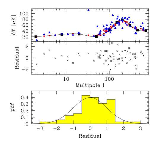
Based on visual inspection of the data, it has been suggested that all CMB measurements cannot be consistent with any model, since some measurements disagree with others on a comparable angular scale. Although we saw above that the $\chi^{2}$-value is acceptable, the distribution of residuals could in principle be non-Gaussian with the a few severe outliers being averaged down beyond recognition in the $\chi^{2}$-calculation. To investigate this possibility, we fit a 10-parameter model with no underlying physical model to the data. Our model curve is simply a cubic spline interpolated between 10 grid points. Figure 10 shows the 65 residuals $(d_{i}-\langle d_{i}\rangle)/\sigma_{i}$, ignoring calibration errors, and reveals no striking outliers at all.

This fit gives a $\chi^{2}\approx 67$ ignoring calibration errors, i.e., even lower than for the CMB case. In view of footnote 1, we repeated this test with merely six spline points. This gave $\chi^{2}\approx 95$ for logarithmically equispaced spline points, but as low a $\chi^{2}$ as before when more points were shifted to be near the 1st acoustic peak.

In the future, as CMB data gets still better, one would expect the correct physically based model to provide a substantially better fit than “any old smooth curve” with the same number of free parameters. Until then, i.e., until our physical theory provides the most economical explanation of the observations, we cannot interpret the good fit of the model to the data as overwhelming evidence that our theory is correct.

Figure 10.— Residuals. The top panel shows a cubic spline interpolated between 10 equispaced grid points (large squares) that are adjusted vertically to make the window function convolved curve (small squares) fit the observations (triangles) as well as possible. The middle panel shows the residuals $(d_{i}-\langle d_{i}\rangle)/\sigma_{i}$, the differences between the triangles and small squares in units of the error bars. The bottom panel shows a histogram of these residuals compared with a unit Gaussian. The reduced $\chi^{2}$-value is simply the second moment of this distribution.

4. CONCLUSIONS

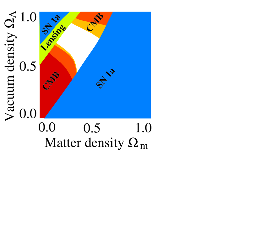
We have presented a method for rapid calculation of large numbers of CMB models and used it to jointly constrain 10 cosmological parameters from current CMB data. Our results on individual parameters are summarized in Table 2. Arguably the most interesting constraints at this point are those on the geometry of spacetime, summarized in Figure 11. This figure zooms in on the upper left quarter of Figure 6 and shows the joint constraints on $\Omega_{\rm m}$ and $\Omega_{\Lambda}$ from a variety of astrophysical observations. The SN 1a constraints are from White 1998, combining the data from both search teams (Perlmutter et al. 1998; Riess et al. 1998; Garnavich et al. 1998). As can be seen, the CMB and SN 1a constraints imply a positive cosmological constant ($\Omega_{\Lambda}>0$) when combined. If the Falco et al. (1998) constraints from gravitational lens statistics are included, the allowed region in parameter space is further reduced.

This claim that $\Omega_{\Lambda}>0$ is of course old hat (Kamionkowski & Buchalter 2000), originally being made over a year ago (see Sahni & Starobinsky 2000 for a recent review). What is new here, and quite striking, is its robustness. Since the first such joint analysis (White 1998), the number of CMB band power measurements has roughly doubled, with experiments such as Toco, Python V, Viper and Boomerang greatly improving the accuracy on acoustic peak scales. In addition, the CMB treatments has been gradually refined; for example, several groups have added calibration errors and this analysis has weakened the constraints further by fitting for 10 parameters jointly. Yet despite these major improvements in both data and modeling, the cosmological constant remains alive and well, stubbornly refusing to vanish.

                                                                

Figure 11.— Constraints in the $\Omega_{\rm m}-\Omega_{\Lambda}$ plane. The regions in the $(\Omega_{\rm m},\Omega_{\Lambda})$-plane that are ruled out by our analysis at $2\sigma$ using all the data are shown using no priors (red/dark grey), the prior $h=0.65\pm 0.07$ (orange/grey), and the additional nucleosynthesis constraint $h^{2}\Omega_{\rm b}=0.02$ (light orange/light grey). The SN 1a constraints are from White (1998) and the lensing constraints are from Falco et al (1998). The CMB contours for $\Omega_{\rm m}<0.2$ are extrapolations.

Since CMB data is likely to continue to improve at a rapid pace, with exciting new balloon, interferometer and satellite data just around the corner, it will be important to further improve on the type of analysis that we have presented here. There are a number of areas in which the accuracy off our treatment can be improved:

• The problem of regenerated power from very early reionization can be eliminated by explicitly looping over $\tau$ for the high $\l$ models in Step 1 instead of using the $e^{-2\tau}$ suppression approximation.

• In Steps 1 and 2, the effect of gravitational lensing can be included.

• In Steps 1 and 2, further speed-up can be attained by taking advantage of the fact that the tensor fluctuations are essentially independent of $\omega_{\nu}$ as long as the total dark matter density $\omega_{\rm cdm}+\omega_{\nu}$ stays constant.

• The accuracy in Step 2 can probably be further improved by using some form of morphing technique as suggested by Sigurdson & Scott (2000). The basic idea is to interpolate not the power spectrum itself but some cleverly chosen parametrization thereof. We have done this to a certain extent by computing and interpolating the amount by which the acoustic peaks should be shifted sideways, but more ambitious reparametrizations are clearly possible.

• In Step 3, the likelihoods can be computed more accurately by incorporating non-Gaussianity corrections as in Bond, Jaffe & Knox (1998) or Bartlett et al. (1999) and by including correlations between different data points. The former is particularly important for upper limits, which were simply excluded from the present analysus. The latter includes correlations between different experiments that overlap in sky coverage and angular scale. Calibrations can be treated as multiplicative parameters to be marginalized over (as in Dodelson & Knox 2000) rather than as correlated noise (our approximation is accurate as long as the relative calibration errors are much less than unity).

• Step 3 should ideally use the exact band power window functions. Unfortunately, most window functions available in the literature are variance window functions, and using them as band-power window functions is an approximation which is not always good. Experimentalists are strongly encouraged to publish their band power window functions!

• The overall accuracy of our technique can be improved with brute force, by computing a finer grid of models in step 1. Indeed, the errors introduced in Step 2 can in principle be continuously reduced toward zero by refining the $(\omega_{\rm cdm},\omega_{\rm b},\omega_{\nu})$-grid for low $\l$ and shifting the splicing point upwards from $\l\sim 100$.

• The accuracy in Step 4 can be improved by integrating instead of maximizing when marginalizing. This will make a difference mainly early on when the 10-dimensional probability distribution in parameter space is widely extended and differs greatly from a multivariate Gaussian distribution. If this integration approach is used, it should be applied even for the normalizations $A_{s}$ and $A_{t}$, for consistency.

A second general area of improvement will be to include more prior information than Hubble parameter measurements and nucleosynthesis constraints. As data improves in a wide variety of areas, this will not only help break parameter degeneracies, but also allow important cross-checks. A very large number of such multi-dataset studies have been carried out in the past (Bahcall et al. 1999 and Bridle et al. 1999 provide good recent entry points into the literature), but rarely for more than a few parameters at a time. Here is a necessarily incomplete list of such constraints:

• Measurements of the matter power spectrum and its time-evolution $P(k,z)$ from galaxy redshift surveys.

• Measurements of $P(k,z)$ from weak gravitational lensing (e.g., Narayan & Bartelmann 1996)

• Measurements of $P(k,z)$ from the abundance of galaxy clusters (e.g., Carlberg 1997; Bahcall & Fan 1998; Eke et al. 1998.)

• Constraints om $P(k)$ from peculiar velocity measurements (e.g., Zehavi & Dekel 1999).

• Limits on $(h,\Omega_{\rm k},\Omega_{\Lambda})$ from SN 1a.

• Limits on $(h,\Omega_{\rm k},\Omega_{\Lambda})$ from lens statistics (e.g., Kochanek 1996; Falco et al. 1998; Bartelmann et al. 1998; Helbig 1999)

• Limits on $(h,\Omega_{\rm k},\Omega_{\Lambda})$ from limits on the age of the Universe and various other classical cosmological tests (Peebles 1993). For instance SZ cluster distance measurements provide promising new constraints of this type (Reese et al. 2000).

• Direct measurements of $\Omega_{\rm m}$ and the baryon fraction $\Omega_{\rm b}/\Omega_{\rm m}$ from cluster studies (Carlberg et al. 1999; White et al. 1993; Danos & Pen 1998; Cooray 1998)

Finally, adding more physics can both weaken and tighten constraints. Adding further parameters (say an equation of state for a scalar field component) can weaken constraints on other semi-degenerate parameters. On the other hand, adding an astrophysical model for, say, how $\tau$ depends on the other parameters can substantially tighten constraints (Venkatesian 2000).

In conclusion, as CMB experimentalists continue to forge ahead, CMB theorists will need to work hard to keep up.

The authors wish to thank Lloyd Knox for helpful comments about calibration errors and Angélica de Oliveira-Costa, Mark Devlin, Charley Lineweaver and Amber Miller for useful discussions. Support for this work was provided by NSF grant AST00-71213, NASA grant NAG5-9194, the University of Pennsylvania Research Foundation, and Hubble Fellowships HF-01084.01-96A and HF-01116.01-98A from STScI, operated by AURA, Inc. under NASA contract NAS5-26555.

A. Conditional marginalization

In this Appendix, we show that maximizing is equivalent to integrating when marginalizing multidimensional Gaussians in arbitrary dimensions. Although this useful property is undoubtedly derived in the statistics literature, we present a brief derivation here for completeness.

A multivariate Gaussian distribution in $n$ dimensions takes the form

$$f({\bf x})=(2\pi|{\bf C}|)^{-n/2}e^{-{1\over 2}({\bf x}-\bar{\bf x})^{t}{\bf C}^{-1}({\bf x}-\bar{\bf x})},$$ (A1)

where $\bar{\bf x}$ is the mean vector and ${\bf C}$ is the $n\times n$ covariance matrix. Let us partition the $n$ parameters in ${\bf x}$ into two subsets ${\bf y}$ and ${\bf z}$ of size $n_{x}$ and $n_{y}$ ($n_{x}+n_{y}=n$) and write

$${\bf x}\equiv\left({\bf y}\atop{\bf z}\right),\quad{\bf C}^{-1}=\left(\begin{tabular}[]{cc}${\bf D}$&${\bf E}$\\ ${\bf E}^{t}$&${\bf F}$\end{tabular}\right).$$ (A2)

We can now define a probability distribution for ${\bf y}$ in two different ways, by either integrating or maximizing over ${\bf z}$:

$$f_{\rm int}({\bf y})\equiv\int f({\bf x})d^{n_{z}}z,$$ (A3)

$$f_{\rm max}({\bf y})\equiv c\max_{{\bf z}}f({\bf x}),$$ (A4)

where the normalization constant $c$ is chosen so that $f_{\rm max}$ integrates to unity. Maximizing $f$ is equivalent to minimizing the quadratic form $({\bf x}-\bar{\bf x})^{t}{\bf C}^{-1}({\bf x}-\bar{\bf x})$. Inserting equation (A2) and differentiating with respect to ${\bf z}$ shows that this minimum is attained for

$${\bf z}=\bar{\bf z}-{\bf F}^{-1}{\bf E}^{t}({\bf y}-\bar{\bf y}).$$ (A5)

Substituting this back into equation (A4) gives

$$f_{\rm max}({\bf y})\propto e^{-{1\over 2}({\bf y}-\bar{\bf y})^{t}[{\bf D}-{\bf E}{\bf F}{\bf E}^{t}]({\bf y}-\bar{\bf y})},$$ (A6)

i.e., a Gaussian with mean $\bar{\bf y}$ and covariance matrix $[{\bf D}-{\bf E}{\bf F}{\bf E}^{t}]^{-1}$. As is well known, integrating over ${\bf z}$ also gives a Gaussian with mean ${\bf y}$ and a covariance matrix which is simply the upper left submatrix of the full covariance matrix ${\bf C}$. The identity

$$\hskip-19.91684pt\left(\begin{tabular}[]{cc}${\bf D}$&${\bf E}$\\ ${\bf E}^{t}$&${\bf F}$\end{tabular}\right)^{-1}=$$ (A9)

$$\hskip-19.91684pt\left(\begin{tabular}[]{cc}$[{\bf D}-{\bf E}{\bf F}^{-1}{\bf E}^{t}]^{-1}$&$-{\bf D}^{-1}{\bf E}[{\bf F}-{\bf E}{\bf D}^{-1}{\bf E}^{t}]^{-1}$\\ $-{\bf F}^{-1}{\bf E}^{t}[{\bf D}-{\bf E}{\bf F}^{-1}{\bf E}^{t}]^{-1}$&$[{\bf F}-{\bf E}{\bf D}^{-1}{\bf E}^{t}]^{-1}$\end{tabular}\right)$$ (A12)

therefore shows that the covariance matrix is $[{\bf D}-{\bf E}{\bf F}^{-1}{\bf E}^{t}]^{-1}$, i.e., the same as for the maximization case. This proves that $f_{\rm int}=f_{\rm max}$, i.e., that the two methods of marginalization give identical results when the probability distribution is Gaussian. The identity given by equation (A9) is readily proven by simply multiplying the matrices on the left and right hand sides together and verifying that their product is the identity matrix.

REFERENCES

Bahcall, N. A., & Fan, X. 1998, ApJ, 504, 1

Bahcall, N., Ostriker, J. P., Perlmutter, S., & Steinhardt P J 1999, Science, 284, 1481

Bartelmann, M. et al. 19928, A& A, 330, 1

Bartlett, J. G., Blanchard, A., & Douspis, M. 1998, astro-ph/9810318

Bartlett, J. G., Douspis, M., & Blanchard, A. 1999, astro-ph/9903045

Bond, J. R. 1995, Phys. Rev. Lett., 74, 4369

Bond, J. R., Efstathiou, G., & Tegmark, M. 1997, MNRAS, 291, L33

Bond, J. R., & Jaffe, A. H. 1998, Phil. Trans. Roy. Soc. London A, 357, 57

Bond, J. R., Jaffe, A. H., & Knox, L. E. 1998, astro-ph/9808264

Bridle, S. L., Eke, V. L., Lahav, O., Lasenby, A. N., Hobson, M. P.,Cole, S., Frenk, C. S., & Henry, J. P. 1999, MNRAS;310;565

Bunn, E. F., & Sugiyama, N. 1995, ApJ, 446, 49

Bunn, E. F., & White, M. 1997, ApJ, 480, 6

Burles, S., Nollett, K. M., Truran, J. N., & Turner, M. S. 1999, Phys. Rev. Lett., 82, 4176

Carlberg, R. G. et al. 1997, ApJL, 479, 19

Carlberg, R. G. et al. 1999, ApJ, 516, 552

Challinor, A., Lewis, A., & Lasenby, A. 2000, ApJ, 538, 473

Coble, K. A. 1999, astro-ph/9911419

Contaldi, C., Hindmarsh, M., & Magueijo, J. 1999, Phys.

Rev. Lett.;82;2034

Cooray, A. 1998, A&A, 333, L71

de Bernardis, P. et al. 1997, ApJ, 480, 1

de Oliveira-Costa, A. et al. 1998, ApJL, 509, L77

Danos, R., & Pen, U. L. 1998, astro-ph/9803058

Devlin, M. et al. 1998, ApJL, 509, L69

Dodelson, S., & Knox, L. 2000, Phys. Rev. Lett, 84, 3523

Efstathiou, G. 1999, MNRAS, 310, 842

Efstathiou, G., Bridle, S. L., Lasenby, A. N., Hobson, M. P., & Ellis,, R. S. 1999, MNRAS, 303, 47

Efstathiou, G., & Bond, J. R. 1999, MNRAS, 304, 75

Eisenstein, D. J., Hu, W., & Tegmark M 1999, ApJ, 518, 2

Eke, V. R., Cole, S., Frenk, C. S., & Henry, J. P. 1998, astro-ph/9802350

Falco, E. E., Kochanek, C. S., & Munoz, J. A. 1998, ApJ, 494, 47

Freedman, W. 1999, Phyd. Rep., 333, 13

Garnavich, P. M. et al. 1998, ApJ, 509, 74

Gawiser, E., & Silk, J. 1998, Science, 280, 1405

Gawiser, E., & Silk, J. 2000, astro-ph/0002044

Green, A. M., Liddle, A. R., & Riotto, A. 1997, Phys. Rev. D, 56, 7559

Gorski, K. M. et al. 1994, ApJL, 430, L89

Griffiths, L. M., Barbosa, D., & Liddle, A. R. 1999, MNRAS, 308, 854

Hancock, S. et al. 1998, MNRAS, 294, L1

Hannestad, S. 1999, astro-ph/9911330

Helbig, P. 1999, A& A, 350, 1

Herbig, T. et al. 1998, ApJL, 509, L73

Hu, W., Eisenstein, D. J., & Tegmark, M. 1998, Phys. Rev. Lett., 80, 5255

Hu, W., Scott, D., & Silk J 1994, ApJ, 430, 5

Hu, W., & Sugiyama, N. 1996, ApJ, 471, 572

Hu, W., Sugiyama, N., & Silk, J. 1997, Nature, 386, 37

Hu, W., & Tegmark, M. 1999, ApJL, 514, L65

Jungman, G., Kamionkowski, M., Kosowsky, A., & Spergel, D. N. 1996, Phys. Rev. D, 54, 1332

Kamionkowski, M., & Buchalter, A. 2000, astro-ph/0001045

Knox, L. 1999, Phys.Rev. D, 60, 103516

Knox, L. et al. 1998, Phys. Rev. D, 58, 083004

Knox, L., & Page, L. A. 2000, Phys. Rev. Lett., 85, 1366

Kochanek, C. S. 1996, ApJ, 466, 638

Lesgourgues, J., Polarski, D., & Starobinsky, A. A. 1999, MNRAS, 308, 281

Liddle, A. R., & Lyth, D. H. 1992, Phys. Lett. B, 291, 391

Lineweaver, C. H. 1998, ApJL, 505, L69

Lineweaver, C. H., & Barbosa, D. 1998a, A&A, 329, 799

Lineweaver, C. H., & Barbosa, D. 1998b, ApJ, 496, 624

Mauskopf, P. D. et al. 2000, ApJ, 536, L59

Melchiorri, A., Sazhin, M. V., Shulga, V. V., Vittorio, N. 1999a, ApJ, 518, 562

Melchiorri, A. et al. 2000, ApJL, 536, L63

Metcalf, R. B., & Silk, J. 1997, ApJ, 489, 1

Miller, A. D. et al. 1999, ApJ, 524, L1

Narayan, R., & Bartelmann, M. 1996, astro-ph/9606001

Peebles, P. J. E. 1993, Principles of Physical Cosmology (Princeton University Press: Princeton)

Perlmutter, S. et al. 1998, Nature, 391, 51

Peterson, J. B. et al. 2000, ApJ;532;L83

Press, W. H. et al. 1992, Numerical Recipes, 2nd ed. (Cambridge Univ. Press: Cambridge)

Ratra, B. et al. 1999, ApJ, 510, 11

Reese, E. D. et al. 2000, ApJ, 533, 38

Riess, A. G. et al. 1998, Astron. J., 116, 1009

Rocha, G. 1999, astro-ph/9907312

Sahni, V., & Starobinsky, A. 2000, Int.J.Mod.Phys., D9, 373

Seljak, U., & Zaldarriaga, M. 1996, ApJ, 469, 437

Sigurdson, K., & Scott, D. 2000, NewA, 5, 91

Smoot, G. F. et al. 1992, ApJ, 396, L1

Stompor, R., & Efstathiou, G. 1999, MNRAS;302;735

Tegmark, M. 1997a, ApJ, 480, L87

Tegmark, M. 1997b, Phys. Rev. D, 55, 5895

Tegmark, M. 1999a, ApJ, 519, 513

Tegmark, M. 1999, ApJL, 514, L69 (“T99”)

Tegmark, M., & Bunn, E. F. 1995, ApJ, 455, 1

Tegmark, M., Eisenstein, D. J., Hu, W., & de Oliveira Costa, A. 2000, ApJ, 530, 133

Torbet, E. et al. 1999, ApJL, 521, L79

Venkatesan, A. 2000, ApJ, 521, 55

Wadsley, J. W., Hogan, C. J., & Anderson, S. F. 1999, astro-ph/9911394

Wandelt, B. D., Hivon, E., & Gorski, K. M. 1998, astro-ph/9808292

Webster, M. et al. 1998, ApJL, 509, L65

White, M. 1998, ApJ, 506, 495

White, M., & Scott, D. 1996, ApJ, 459, 415

White, S. D. M. et al. 1993, Nature, 366, 429

Wilson, G. W. et al. 1999, astro-ph/9902047

Wright, E. L. 1996, preprint astro-ph/9612006.

Zaldarriaga, M., Spergel, D., & Seljak, U. 1997, ApJ, 488, 1

Zaldarriaga, M., & Seljak, U. 1999, astro-ph/9911219

Zehavi, I., & Dekel, A. 1999, Nature, 401, 252