The entropy and energy of intergalactic gas in galaxy clusters

Abstract

Studies of the X-ray surface brightness profiles of clusters, coupled with theoretical considerations, suggest that the breaking of self-similarity in the hot gas results from an ‘entropy floor’, established by some heating process, which affects the structure of the intracluster gas strongly in lower mass systems. By fitting analytical models for the radial variation in gas density and temperature to X-ray spectral images from the ROSAT PSPC and ASCA GIS, we have derived gas entropy profiles for 20 galaxy clusters and groups. We show that when these profiles are scaled such that they should lie on top of one another in the case of self-similarity, the lowest mass systems have higher scaled entropy profiles than more massive systems. This appears to be due to a baseline entropy of 70-140 ${h_{50}}^{-\frac{1}{3}}$ keV cm² depending on the extent to which shocks have been suppressed in low mass systems. The extra entropy may be present in all systems, but is detectable only in poor clusters, where it is significant compared to the entropy generated by gravitational collapse. This excess entropy appears to be distributed uniformly with radius outside the central cooling regions.

We determine the energy associated with this entropy floor, by studying the net reduction in binding energy of the gas in low mass systems, and find that it corresponds to a preheating temperature of $\sim 0.3$ keV. Since the relationship between entropy and energy injection depends upon gas density, we are able to combine the excesses of 70-140 keV cm² and 0.3 keV to derive the typical electron density of the gas into which the energy was injected. The resulting value of 1-3$\times 10^{-4}{h_{50}}^{\frac{1}{2}}$ cm^-3, implies that the heating must have happened prior to cluster collapse but after a redshift $z\sim$ 7-10. The energy requirement is well matched to the energy from supernova explosions responsible for the metals which now pollute the intracluster gas.

1 Introduction

The hierarchical clustering model for the formation of structure in the universe predicts that dark matter halos should be scaled versions of each other (?). While some energy transfer between dark matter and gas is possible through gravitational interaction and shock heating, simulations suggest that the gas and dark matter halos will be almost self-similar in the absence of additional heating or cooling processes  (?). Comparison of the structure of real galaxy systems with this predicted self-similarity provides an excellent probe of extra physical processes that may be taking place in galaxy clusters and groups.

It has been suggested that specific energy in cluster cores is higher than expected from gravitational collapse and that this may be due to energy injected by supernova-driven protogalactic winds  (?; ?). ? studied the entropy in a small sample of galaxy systems and suggested that the entropy in their cores had been flattened due to energy injection. ? have recently shown that the surface brightness profiles of clusters and groups do not follow the predicted self-similar scaling. Surface brightness profiles of galaxy groups are observed to be significantly flatter than those of clusters, indicating differences in the gas distribution.

Table 1: Some important properties for the sample of 20 galaxy clusters and groups. Systems are listed in order of increasing temperature.

Cluster/Group	R.A.(J2000)	Dec.(J2000)	z	$N_{H}$($10^{20}$ cm-2)	$T$(keV)	$Z$(solar)	Data
HCG 68	208.420	40.319	0.0080	0.90	0.54	0.43	PSPC
HCG 97	356.845	-2.169	0.0218	3.29	0.87	0.12	PSPC
HCG 62	193.284	-9.224	0.0137	3.00	0.96	0.15	PSPC
NGC 5044 Group	198.595	-16.534	0.0082	5.00	0.98	0.27	PSPC
RX J0123.6+3315	20.921	33.261	0.0164	5.0	1.26	0.33	PSPC
Abell 262	28.191	36.157	0.0163	5.4	1.36	0.27	PSPC
IV Zw 038	16.868	32.462	0.0170	5.3	1.53	0.40	PSPC
Abell 400	44.412	6.006	0.0238	9.1	2.31	0.31	PSPC
Abell 1060	159.169	-27.521	0.0124	5.01	3.24	0.27	PSPC+GIS
MKW 3s	230.507	7.699	0.0453	3.1	3.68	0.30	PSPC
AWM 7	43.634	41.586	0.0173	9.19	3.75	0.33	PSPC
Abell 780	139.528	-12.099	0.0565	4.7	3.8	0.23	PSPC+GIS
Abell 2199	247.165	39.550	0.0299	0.87	4.10	0.30	PSPC
Abell 496	68.397	-13.246	0.0331	4.41	4.13	0.31	PSPC+GIS
Abell 1795	207.218	26.598	0.0622	1.16	5.88	0.26	PSPC
Abell 2218	248.970	66.214	0.1710	3.34	6.7	0.20	PSPC+GIS
Abell 478	63.359	10.466	0.0882	13.6	7.1	0.21	PSPC+GIS
Abell 665	127.739	65.854	0.1818	4.21	8.0	0.28	PSPC+GIS
Abell 1689	197.873	-1.336	0.1840	1.9	9.0	0.26	PSPC+GIS
Abell 2163	243.956	-6.150	0.2080	11.0	13.83	0.19	PSPC+GIS

Notes: Positions, hydrogen columns and redshifts are taken from ?, ?, ? and ?. Emission weighted temperatures and metallicities for these systems are taken from ?, ?, ?, ?, ?, ?, ?, ?, ?, ? and ?.

In order to explore this effect further, it is necessary to study the properties of the gas in these systems in greater detail. A particularly interesting property of the gas for this purpose is its entropy, as this will be conserved during adiabatic collapse of the gas into a galaxy system, but is likely to be altered by any other physical processes. For instance preheating of the gas before it falls into the cluster, energy injection from galaxy winds and radiative cooling of the gas in dense cluster cores will all perturb the entropy profiles of clusters from the self-similar model. Analysis of the entropy profiles of virialized systems of different masses should therefore allow the magnitude of such effects to be studied, constraining the possible processes responsible. A key question to answer in this regard is how much energy is involved in any departures from self-similarity of the entropy profiles. The study of ? was not able to address this issue in detail, since the gas was assumed to be isothermal. Here we combine ROSAT PSPC and ASCA GIS data to constrain temperature profiles, allowing a more detailed study of entropy and energy distributions in the intergalactic medium (IGM).

Energy loss from the gas due to cooling flows in the centres of clusters and groups will actually lead to an increase in the gas entropy outside the cooling region  (?). This is because as gas cools out at the centre of the system, gas from a larger radius, which has higher entropy, flows in adiabatically to replace it. However this effect will not be very large unless a significant fraction of the gas in the system cools out, which is not feasible within a Hubble time, even for systems with exceptionally large cooling flows.

Energy injection into the gas will also raise the entropy profiles of systems. This energy injection could occur either before or after the systems’ collapse, but more energy is needed to get the same change in entropy when the gas is more dense  (?). There are several possible processes that might have injected energy into the intracluster medium: radiation from quasars, early population III stars, or energetic winds associated with galaxy formation.

There may also be transient effects on the entropy profiles of systems due to recent mergers. Hydrodynamical simulations suggest that the entropy profiles of systems are flattened and their central entropy raised during a merger, and this will last until the system settles back into equilibrium  (?). In order to look for the effects of extra physical processes, it is advantageous to study a set of systems with a large range in system mass, as these processes will break the expected self-similar scaling relations. In the present paper we examine the properties of the intracluster gas in systems with mean temperatures ranging over a factor of 25, corresponding to virial masses varying by over two orders of magnitude.

2 Sample

The sample selected for this study consisted of 20 galaxy systems ranging from poor groups to rich clusters, with high quality ROSAT PSPC and in some cases ASCA GIS data. Basic properties of these systems are listed in Table 1. The sample was chosen to cover a wide range of system masses but is not a ‘complete’ or statistically representative sample of the galaxy cluster/group population. It is necessary that the systems be fairly relaxed and spherical in order for the assumption of spherical symmetry used in the analysis to be reasonable, and they were selected with this in mind, although it will be seen later that some of the systems are not as relaxed as we had hoped. In general, our sample should be representative of the subset of galaxy systems which is fairly relaxed and X-ray bright. Galaxy systems which are not virialized, or those currently undergoing complex mergers, would be expected to have systematically different properties. Our sample spans the population range from small groups to rich clusters, covering a range in emission weighted gas temperature from 0.5 to 14 keV. It is therefore well-suited to investigating the scale dependence in cluster properties.

3 Data reduction

In general ASCA GIS data were used only where ROSAT PSPC data were insufficient to constrain the models. This was generally the case for systems with temperatures greater than 4 keV but the cutoff can be somewhat higher for high quality ROSAT PSPC data (i.e. Abell 1795 and Abell 2199). In the cases where it is possible to access the consistency of results from ROSAT PSPC and ASCA GIS data it appears that they are in reasonable agreement. The results of fits to ROSAT PSPC data and joint fits to ROSAT PSPC and ASCA GIS data for Abell 1060 are quite similar. The temperature profiles derived from ROSAT PSPC data for Abell 1795 and Abell 2199 are also consistent with the emission weighted temperature obtained by previous authors from ACSA data.

A similar reduction process was applied to the ROSAT and ASCA data for each system. For the ROSAT PSPC, the data were screened to remove periods of high particle background, where the master veto rate was above 170 counts s^-1. The background was calculated from an annulus typically between 0.6-0.7^∘ off-axis. This annulus was moved to larger radii for clusters of large spatial extent, to avoid cluster emission contaminating the background. Point sources of significance greater than 4$\sigma$, together with the PSPC support spokes, were removed and the background in the annulus was extrapolated across the detector using the energy dependent vignetting function.

For the ASCA GIS, the data were screened to to remove periods of high particle background. The following parameters were used to select good data; cut-off rigidity ($COR$) $>$ 6 GeV c^-1; radiation belt monitor count rate $<$ 100; GIS monitor count rate ‘H02’ $<$ 45.0 and $<$ 0.45 x $COR^{2}$ - 13 $\times$ $COR$ + 125. Data were also excluded where the satellite passed through the South Atlantic Anomaly and where the elevation angle above the Earth’s limb was $\leq$ 7.5^∘. The background was taken from the sum of a number of ‘blank sky’ fields screened in the same way as the source data and scaled to have the same exposure time as the observation of the source.

In order to carry out our cluster modelling analysis, spectral image cubes were sorted from the raw data. The ROSAT PSPC cubes had 11 energy bins covering PHA channel 11 to 230, and spatial bins $25^{\prime\prime}$ in size. The ASCA GIS cubes had 24 energy bins spanning PHA channel 120 to 839, and spatial bins $1.96^{\prime}$ in size. Only data from within the PSPC support ring were used. For all systems this encompassed the great majority of the detectable ROSAT flux. PSPC radial surface brightness profiles were used to set the extraction radius in each case to restrict data to the region where diffuse emission is apparent above the noise. ASCA data were extracted from a regions similar in size to the corresponding PSPC dataset. Point sources were removed from the PSPC cubes. In the case of ASCA, the poor PSF makes this infeasible, however none of our targets includes bright hard sources which might seriously affect our GIS analysis.

The data cubes were background subtracted and then normalized to count s^-1. The cubes were not corrected for vignetting as this would invalidate the Poisson statistics assumed in our subsequent analysis. Instead the vignetting was taken account of when fitting the data.

4 Cluster Analysis

Each of the 20 galaxy clusters and groups in the sample has a high quality ROSAT PSPC observation available. For several of the clusters, as detailed in Table 1, ASCA GIS data were also used. The use of ASCA GIS data is desirable for high temperature systems, as the GIS has a bandpass that extends to much higher energies than the PSPC.

Our cluster analysis works by fitting analytical models to the spectral images from one or both of the instruments. The models parametrize either the gas density and temperature, or the gas density and dark matter density, as a function of radius. Dark matter as far as these models are concerned is all gravitating matter apart from the X-ray emitting gas. Under the assumption of hydrostatic equilibrium and spherical symmetry, the equation

$$M(r)=-\frac{T(r)r}{G\mu}\left[\frac{dln\rho}{dlnr}+\frac{dlnT}{dlnr}\right]$$ (1)

is satisfied  (?), and therefore the dark matter density distribution can be calculated from the temperature distribution or vice versa, if the gas density distribution is known. The models assume that the systems are spherically symmetric and the dark matter models also assume hydrostatic equilibrium. It is also assumed that the densities and temperatures can be reasonably represented by analytical functions and that the plasma is single phase (i.e. each volume element contains gas at just a single temperature). The density in all the models is represented by a core-index function of the form:

$$\rho(r)=\rho(0)\left[1+\left(\frac{r}{r_{c}}\right)^{2}\right]^{-\frac{3}{2}\beta}$$ (2)

where $r_{c}$ is the core radius and $\beta$ is the density index. This has been shown to be a good fit to observations of clusters  (?). The temperature profile is parametrized using a linear function of the form:

$$T(r)=T(0)-{\alpha}r$$ (3)

where $\alpha$ is the temperature gradient. In the case of the dark matter density parametrization we use a profile derived from numerical simulations  (?) of the form:

$$\rho_{DM}(r)=\overline{\rho}_{DM}\left[x(1+x)^{2}\right]^{-1}$$ (4)

where $x=r/r_{s}$ and $r_{s}$ is a scale radius. Combining this with in gas density distribution results in the total mass density distribution which along with a temperature normalization parameter $T(0)$ allows the gas temperature distribution to be calculated. The metallicity of the gas is parametrized as a linear ramp in a similar way to the gas temperature. The metallicity gradient was fixed at zero where only ROSAT PSPC data were used. The aim of using models that parameterize the gas temperature both directly and indirectly, is to more fully explore the parameter space available and so try to reduce the problem of implicit bias associated with using a specific analytical model.

Our analysis also allows an optional extra cooling flow component to be included in the models. This takes over from the normal density and temperature parametrizations inside a cooling radius which is a fitted parameter of the model. The density increases and the temperature decreases as a powerlaw from the values at the cooling radius to the

Table 2: Main parameters of the best fitting models for the sample. The temperature and dark matter models have slightly different parameters. An asterisk in the CF column specifies that the model used a cooling flow component.

Cluster/Group	$\rho(0)$	$r_{c}$	$\beta$	T(0)	$\alpha$	$\rho_{DM}$(0)	$r_{s}$	CF
	(cm-3)	(arcmin)		(keV)	(keV arcmin-1)	(amu cm-3)	(arcmin)
HCG 68	0.0161	0.28	0.44	0.86	0.036	-	-
HCG 97	0.119	0.04	0.41	1.05	0.020	-	-
HCG 62	0.138	0.03	0.36	1.49	0.023	-	-	*
NGC 5044 Group	0.009	1.66	0.49	1.21	-0.005	-	-	*
RX J0123.6+3315	0.121	0.10	0.43	1.50	0.022	-	-	*
Abell 262	0.00725	1.45	0.39	1.45	-0.081	-	-	*
IV Zw 038	0.00116	2.77	0.38	2.39	0.043	-	-
Abell 400	0.00189	3.83	0.51	1.68	-0.014	-	-
Abell 1060	0.00319	7.35	0.70	3.28	-	0.189	4.92	*
MKW 3s	0.0270	0.64	0.53	4.93	0.255	-	-
AWM 7	0.00418	5.53	0.60	2.88	-0.094	-	-	*
Abell 780	0.00855	1.69	0.67	4.05	-0.203	-	-	*
Abell 2199	0.00990	2.20	0.61	3.13	-0.103	-	-
Abell 496	0.00504	3.24	0.64	6.34	0.140	-	-	*
Abell 1795	0.0245	0.75	0.57	6.74	-	0.109	2.47
Abell 2218	0.00508	0.90	0.56	10.99	0.968	-	-
Abell 478	0.0236	0.84	0.62	8.318	0.445	-	-	*
Abell 665	0.00754	0.73	0.52	13.76	1.465	-	-
Abell 1689	0.0290	0.60	0.73	12.31	0.002	-	-	*
Abell 2163	0.00819	1.17	0.62	11.50	0.580	-	-

centre, with fitted powerlaw indices. In the case of models that parametrize dark matter density rather than temperature, no explicit cooling flow temperature parameterization is needed, as the model permits the derived temperature to drop at small radii. The density and temperature powerlaws were flattened inside $r$ = 10 kpc, to prevent them going to infinity.

The models described above, specify the density, temperature and metallicity at each point in the cluster. Using the MEKAL hot coronal plasma code  (?) it is then possible to compute the emission from each volume element, and to integrate up the X-ray emission for each line of sight through the cluster. This predicted emission is then convolved with the response of the instrument in order to calculate the predicted observation for the instrument. Standard energy responses and vignetting functions were used for each instrument. Position and energy dependent point spread functions were used. The ASCA GIS PSF is obtained by interpolating between several observations of Cyg X-1 at various positions on the detector  (?). After folding the projected data through the spatial and spectral response of the instrument and applying vignetting, a predicted spectral image is obtained. This is then compared with the observed spectral image, and the model parameters altered iteratively, until a best fit is obtained. In cases where both ROSAT PSPC and ASCA GIS data were used, the model was fitted to both datasets simultaneously. This required careful adjustment to take account of differences in the response and pointing accuracy of the different telescopes. To achieve this the ASCA GIS dataset was repositioned so that the models fitted to same position as the ROSAT PSPC. Our analysis allows renormalization factors to be applied to the model predictions to take account of gain variations between the different instruments. A maximum likelihood method was used to compare the data with the model predictions, as there are low numbers of counts in many bins of the spectral image, and hence $\chi^{2}$ is inappropriate. Further details of this cluster analysis technique can be found in ?.

Because of the large number of parameters in our models, typically $\geq 10$, the fit space for the models can be complicated. It is necessary to find the global minimum of the fit statistic in the fit space. Two complementary methods were used to minimize the fit statistic and find the best model fit. Initially a genetic algorithm  (?) was used to try to get close to the global minimum in the fit space. This works by creating a population of solutions randomly distributed across the fit space. These solutions are then allowed to reproduce, by mutation (altering parameters) or sexual reproduction (crossing over or averaging parameters between parent solutions) with more chance of reproduction being given to solutions giving better fits. Solutions with the poorest fits are killed off as new solutions are created, and in this way the fitness of the population improves through ‘natural selection’. This method is less likely to get trapped in local minima in the fit space than conventional descent methods. Once the locality of the global minimum is found a more conventional modified Levenberg-Marquardt method  (?) was used to find the exact position of the minimum in the fit space. By using these two methods in conjunction the global minimum is much more likely to be found.

Confidence intervals for the model parameters were calculated by perturbing each parameter in turn from its best fit value, while allowing the other fitted parameter to optimize, until the fit statistic increased by 1. This was done in the positive and negative directions for each fitted parameter, to obtain the parameter offsets that correspond to this change in the fit statistic. A change in the fit statistic of 1 corresponds to 1$\sigma$ confidence. All errors quoted below are 1$\sigma$.

The models used to derive the results presented below were the temperature or dark matter model for each system that gave the best fit to the data. Once the fitted models had been obtained it was possible to derive many different system properties, including total gravitating mass and gas entropy profiles. Throughout the following analysis we adopt $H_{0}$=50 km s^-1 Mpc^-1 and $q_{0}$ = 0.5 , and show the $H_{0}$ dependence of key results in terms of $h_{50}$ (=$H_{0}$/50).

Figure 1: $\beta$ plotted against system temperature for 20 galaxy clusters and groups. The dotted line shows $\beta=\frac{2}{3}$.

5 Results

The main parameters of the best fit model for each system in the sample are shown in Table 2. In this paper we will concentrate on the departures from self-similarity in these systems and specifically the entropy and energy of the intergalactic gas. A further paper is in preparation which deals with other results from our sample. Before deriving entropy profiles for the sample, the fitted parameters of the models themselves were studied to see if they deviated from self-similar scaling predictions. The $\beta$ parameter in Equation 2, which is essentially equivalent to the $\beta_{fit}$ parameter often used to fit X-ray surface brightness profiles, showed a strong departure from self-similarity in the low mass systems. This is shown in Fig. 1. It can be seen that the gas density profiles of the systems in the sample are not simply scaled versions of one another. High mass systems have $\beta$ values around the canonical value of $\frac{2}{3}$. Low mass systems have significantly flatter gas density profiles, with $\beta$ dropping to $\sim 0.4$ for the galaxy groups which agrees well with the ? study of the surface brightness profiles of galaxy groups. This is also supported by most recent studies of galaxy clusters  (?; ?) and is predicted by recent simulations of energy injection into clusters  (?; ?). However, ? fitted two component core-index models to the surface brightness profiles of a sample of galaxy clusters and found no dependence of $\beta_{fit}$ on temperature. Our analysis also allows for the presence of a second central component associated with a cooling flow, where necessary. However the apparent conflict between Fig. 1 and the results of ? is resolved by the fact that their sample did not extend much below 3 keV, and it can be seen from the figure that no significant trend above 3 keV is seen in our sample. It should be noted that the $\beta$ values we derive parametrize 3-dimensional gas density and are not directly comparable to $beta$ values that parameterize X-ray surface brightness as isothermality has not been assumed. In general the $beta$ values that we derive are slightly lower than those derived from surface brightness profiles  (?; ?). Some difference is to be expected as we do not assume isothermality.

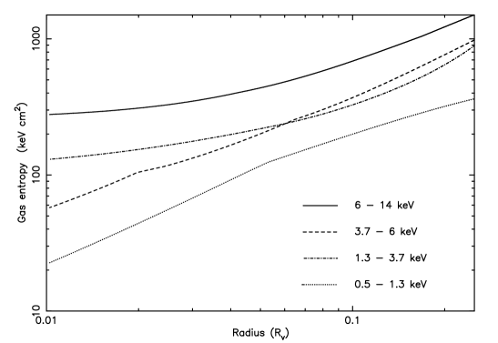
Figure 2: Mean gas entropy against radius scaled to the virial radius for the sample, grouped by system temperature. The solid line represents the five most massive systems (6-14 keV), through dashed (3.7-6 keV) and dash-dot (1.3-3.7 keV), to dotted (0.5-1.3 keV) for the lowest mass systems. The discontinuities in slope seen in some mean profiles, occur at the outer boundary of a central cooling flow component in the fitted model.

Figure 3: Gas entropy at 0.1R_v against system temperature for 20 galaxy clusters and groups. The dotted line is a S$\propto$T fit to the systems above 4 keV excluding Abell 665 and Abell 2218 (see discussion in text). The dashed line is a constant entropy floor of 139$\pm$7 keV cm² fitted to the four lowest temperature systems.

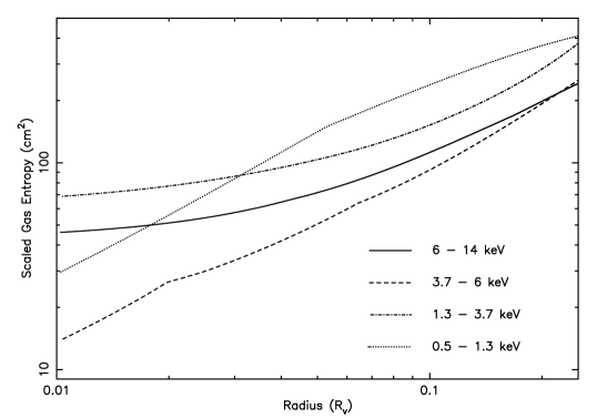
Figure 4: Mean gas entropy scaled by $T^{-1}(1+z)^{2}$ against radius scaled to the virial radius for the sample, grouped by system temperature. The solid line represents the five most massive systems (6-14 keV), through dashed (3.7-6 keV) and dash-dot (1.3-3.7 keV), to dotted (0.5-1.3 keV) for the lowest mass systems.

Figure 5: Scaled entropy at 0.1R_v against system temperature for 20 galaxy clusters and groups. The dotted line shows the weighted mean scaled entropy of 54$\pm$3 cm² for the systems above 4 keV excluding Abell 665 and Abell 2218 (see discussion in text).

5.1 Excess entropy

Gas entropy profiles as a function of radius were derived for the 20 systems. It is convenient to define ‘entropy’ in terms of the observed quantities, ignoring constants and logarithms, as

$$S=\frac{T}{n_{e}^{2/3}}$$ (5)

where $T$ is the gas temperature in keV and $n_{e}$ is the gas electron density. The radius axis of each profile was scaled to the virial radius of the system, calculated using the formula

$$R_{v}=2.57\left(\frac{T}{5.1\rm{keV}}\right)^{\frac{1}{2}}(1+z)^{-\frac{3}{2}}\rm{Mpc}$$ (6)

derived from numerical simulations  (?). The profiles were then grouped together by temperature and averaged in order to improve the clarity of the figures and to high-light their temperature dependence. The mean entropy profiles for groups of systems with similar temperatures are shown in Fig. 2. Each line in the figure is the average of the profiles of 5 systems in a certain temperature range. It can be seen that the most massive systems have the highest entropy gas. The gas entropy in all systems shows a general increase with radius. This is to be expected, as if the entropy declined with radius the gas would be convectively unstable. The profiles are similar to those seen in hydrodynamical simulations such as those of ? and ?. At small radii the profiles are dominated by the effects of cooling flows in many systems, resulting in a lowered central gas entropy.

To investigate the dependence of gas entropy on system temperature, the entropy at 0.1 $R_{v}$ has been plotted against the mean system temperature for each individual system. This is shown in Fig. 3. A radius of 0.1 $R_{v}$ was chosen to be close to the cluster centre (where shock heating is minimized), but to lie outside the cooling region in all systems. It can be seen that for the high temperature systems the gas entropy is will appears to follow the expected $S\propto T$ scaling. The dotted line is a powerlaw with a slope of unity fitted to the systems with mean temperatures above 4 keV. It is clear that the low temperature systems deviate from this trend and appear to flatten out to a constant entropy floor. The dashed line is a constant gas entropy fitted to the four lowest temperature systems and has a value of 139$\pm$7 ${h_{50}}^{-\frac{1}{3}}$ keV cm². This effect has previously been noted by ? using isothermal assumptions.

In order to study the departures from self-similar scaling in more detail, the profiles were scaled by a factor $T^{-1}(1+z)^{2}$, where $T$ is the integrated system temperature and $z$ is the system redshift, and overlayed. The $T^{-1}$ scaling should remove the effects of system mass, as from Equation 5 it can be seen that ‘entropy’ is directly proportional to gas temperature. The $(1+z)^{2}$ scaling removes the effect of the evolution of the mean density of the Universe, which has a $(1+z)^{3}$ dependence, and results in systems that form at higher redshifts being more dense. This assumes that the systems formed at the redshift of observation. The net result of this scaling is that the profiles should fall on top of each other in the case of simple self-similar scaling. The profiles were then grouped as before, resulting in the mean profiles shown in Fig. 4.

It can be seen from Fig. 4 that the scaled entropy profiles of the sample do not coincide. In general the less massive systems have higher scaled entropy profiles, with galaxy groups having the highest scaled entropy values. This can be seen more clearly in Fig. 5, where the scaled entropy at 0.1 $R_{v}$ has been plotted against the mean system temperature. The lower mass systems clearly show an excess in scaled entropy over the high mass systems. In particular, systems with temperatures above 4 keV appear to have a roughly constant scaled entropy, while for systems with temperatures below 4 keV the scaled entropy increases with decreasing temperature. A radius of 0.1 $R_{v}$ was used as this lies outside the cooling flow regions of all the systems.

Three of the systems stand out as being somewhat different from the general trend. These are the clusters Abell 2218 and Abell 665, and the group IV Zw 038 (also known as the NGC 383 group). As well as lying above the trend in Fig. 5, they also show unusual scaled entropy profiles having the highest central scaled entropies in the sample. Our fits indicate that both of the clusters have very high temperature gradients, a linear temperature fit (Equation 3) gives $\sim$6.2 keV Mpc^-1 for Abell 665 and $\sim$4.3 keV Mpc^-1 for Abell 2218, which are which make them very unusual compared to the rest of our sample. Neither of these clusters has a significant cooling flow, and both Abell 2218  (?) and Abell 665  (?) have been suggested as being on-going or recent mergers. IV Zw 038 has a somewhat lower temperature gradient of $\sim$1.5 keV Mpc^-1 although this is still large, given the low mean temperature of this system. ? have studied the X-ray emission of IV Zw 038 and concluded that it is fairly relaxed. However ? studied the distribution of galaxies around IV Zw 038 and concluded that the system is highly substructured. It therefore appears that IV Zw 038 may also be an ongoing or recent merger. As noted previously, transient flattening of entropy profiles during mergers is seen in hydrodynamical simulations  (?).

A mean value was calculated for the scaled entropy of the systems with temperatures above 4 keV. The clusters Abell 2218 and Abell 665 were excluded from this calculation due to their deviant behaviour. A weighted mean value of 54$\pm$3 cm² was calculated. This was subtracted off the entropies of the 12 systems with temperatures below 4 keV to calculate their excess entropy. This (unscaled) excess entropy is plotted against system temperature in Fig. 6. The excess entropy shows no trend with temperature and has a mean value of 68$\pm$12 keV cm². This value drops slightly to 67 keV cm² if IV Zw 038 is excluded. To investigate whether the excess gas entropy varies with radius this procedure was repeated for radii from 0.0-0.2 $R_{v}$. It was not possible to extend this analysis beyond 0.2 $R_{v}$ reliably, because the data for the lowest mass systems does not extend that far due to their low surface brightness. The variation of mean excess entropy against radius is shown in Fig. 7.

The mean excess entropy appears to be constant outside a central cooling region which principally affects the innermost point in the figure. When only the three systems without central cooling are plotted, the result is the diamond in Fig. 7. This seems to confirm that the excess entropy is distributed fairly evenly with radius and it is the effect of cooling flows that causes the radial dependence seen in Fig. 7. The cooling radii for these systems are $<$ 0.1 $R_{v}$ and it is to be expected that within cooling flows large amounts of entropy will be lost as the gas cools. The asymptotic value of excess entropy outside the cooling region is $\sim$70 ${h_{50}}^{-\frac{1}{3}}$ keV cm².

Figure 6: Excess entropy at $0.1R_{v}$ against system temperature for 12 systems with temperatures below 4 keV. The dotted line shows the weighted mean value of 68$\pm$12 keV cm².

Figure 7: Mean excess gas entropy against radius for the 12 systems with mean temperatures below 4 keV. The diamond shows the central mean excess entropy for the 3 systems without significant cooling.

To investigate whether cooling flows are having any impact on the entropy profiles of the systems at large radii (cf. discussion of the ? result in the introduction), excess entropy at 0.1 R_v was compared to cooling flow size. It was possible to derive reliable cooling flow mass deposition rates for 8 of the 12 systems with temperatures below 4 keV (the remaining systems were consistent with no cooling within errors or were not constrained by the analysis). This was done using the equation,

$$\stackrel{{\scriptstyle.}}{{M}}(i)=\frac{L(i)-[\Delta{h(i)}+\Delta{\phi(i)}]\sum_{i^{\prime}=1}^{i^{\prime}=i-1}\stackrel{{\scriptstyle.}}{{M}}(i^{\prime})}{h(i)+f(i)\Delta{\phi}}$$ (7)

from ?, where $\stackrel{{\scriptstyle.}}{{M}}(i)$ is the mass deposition rate, $L(i)$ is the luminosity, $h(i)$ is the thermal energy per particle, and $\phi(i)$ is the gravitational energy per particle in the radial bin $i$. The $\Delta$ symbols represent a change in a quantity across a radial bin. $f(i)$ is a factor that can be calculated to allow for the volume averaged radius at which the mass drops out in the radial bin $i$. A value of 1 was used for $f(i)$ for simplicity, which is consistent with previous analysises  (?). By integrating this equation out from the centre of the system the mass deposition rate within any radius can be calculated. The radius at which the cooling time equals the Hubble time, 1.3 $\times$ 10¹⁰yrs for $H_{0}$ = 50 km s^-1 Mpc^-1, was used for consistency with previous work.

Table 3: Cooling flow mass deposition rates derived in this work compared to rates from the literature. Asterisks indicate systems shown in Fig. 8. The dashes in the second column indicate that no reliable value could be derived from our analysis and the dashes in the third column indicate that no value was available in the literature.

Cluster/Group	$\dot{M}$ this work	$\dot{M}$ literature
	($M_{\odot}yr^{-1}$)	($M_{\odot}yr^{-1}$)
HCG 68$\ast$	$0.7^{+1.3}_{-0.5}$	-
HCG 97$\ast$	$4^{+19}_{-3}$	-
HCG 62	$6^{+95}_{-6}$	$\sim$10
NGC 5044 Group$\ast$	$25^{+20}_{-3}$	20-25
RX J0123.6+3315$\ast$	$18^{+6}_{-3}$	-
Abell 262	-	-
IV Zw 038	-	$27^{+4}_{-3}$
Abell 400$\ast$	$7.2^{+0.5}_{-0.5}$	$0^{+28}_{-0}$
MKW 3s$\ast$	$50^{+5}_{-5}$	$175^{+14}_{-46}$
Abell 1060	-	$15^{+5}_{-7}$
AWM 7$\ast$	$65^{+21}_{-21}$	$41^{+6}_{-6}$
Abell 780$\ast$	$274^{+25}_{-24}$	$264^{+81}_{-60}$
Abell 496	$105^{+17}_{-16}$	$134^{+58}_{-85}$
Abell 2199	$243^{+13}_{-10}$	$154^{+18}_{-8}$
Abell 1795	-	$321^{+166}_{-213}$
Abell 2218	-	$66^{+76}_{-30}$
Abell 478	$974^{+162}_{-132}$	$616^{+63}_{-76}$
Abell 665	-	$0^{+206}_{-0}$
Abell 1689	$470^{+70}_{-180}$	$0^{+398}_{-0}$
Abell 2163	-	$0^{+256}_{-0}$

Note: The cooling flow mass deposition rates from the literature were obtained from ?, ?, ? and ?.

The cooling flow mass deposition rates derived from our analysis for the whole sample are listed in Table 3 along with values taken from the literature. In general there is good agreement between the values we derive and previously derived values. The cooling flow mass deposition rates for the 8 systems with temperatures below 4 keV were then scaled by $T^{-3/2}$, which is proportional to $M^{-1}$, to scale the cooling flows to the system size. The scaled mass deposition rates are therefore proportional to the fraction of the cluster mass that is cooling out per year. These scaled mass deposition rates have been plotted against excess entropy in Fig. 8. It can be seen that there is no appreciable correlation between excess entropy and scaled mass deposition over more than an order of magnitude range in scaled mass deposition rate. The weighted mean value for the excess entropy in the systems with no measurable cooling is 67 $\pm$ 15 keV cm², almost identical to the mean for all the systems with temperatures below 4 keV. These results confirm that cooling is not driving the trend seen in Fig. 5.

Figure 8: Excess entropy at $0.1R_{v}$ against cooling flow mass deposition rate scaled by $T^{-3/2}$ for 8 systems with temperatures below 4 keV.

5.2 Excess energy

? assumed that their systems were isothermal, and so were unable to measure the extra energy in the IGM which gives rise to this excess entropy. Their analysis was therefore based on a rough estimate of the likely energy injection based on the assumption that it was caused by supernova-driven galactic winds. Here, because of our spatially resolved temperature profiles, we can actually attempt to measure the injected energy and then compare it to the energy expected from galactic winds or other heating mechanisms.

Figure 9: Mean binding energy per particle of the central 0.004$M_{200}$ of gas against system temperature for 20 galaxy clusters and groups. The dashed line shows a $E\propto T$ line fitted through the systems with mean temperatures greater than 4 keV. The solid line shows our best estimate of the $E=AT-\Delta{E}$ relationship (for $\Delta{E}=0.44$ keV) with 1$\sigma$ errors (dotted).The dot-dashed line is the result obtained when the unreliable point for the cluster Abell 400 is included in the fit (see discussion in text).

The excess energy is composed of two parts: extra thermal energy, and reduced gravitational binding energy. Due to the fact that our data do not extend beyond 0.2 $R_{v}$ for the lowest mass systems, it was not possible to calculate the total binding energy of the gas within the virial radius for the entire sample, and since energy injection will change the gas distribution, considering the binding energy of the gas within a fixed fraction of the virial radius will be misleading. Instead, we investigate the binding energy of gas constituting a fixed fraction of the virial mass of each system. If the gas distributions of the systems were self-similar, this would translate into gas within a fixed fraction of the virial radius, but it can be seen from Fig. 1 the gas distributions of the systems are not self-similar. In order to calculate the virial masses of the systems from their mean temperatures the formula

$$M_{200}=10^{15}\left(\frac{T}{5.1\rm{keV}}\right)^{\frac{3}{2}}(1+z)^{-\frac{3}{2}}\rm{M}_{\odot}$$ (8)

was used  (?), which is derived from numerical simulations. A fixed fractional gas mass of 0.004 $M_{200}$ was used, which was found to correspond to a fraction of the virial radius between 0.064 and 0.226 for the systems in the sample.

The mean binding energy per particle of the central 0.004 $M_{200}$ of gas for the sample is plotted against temperature in Fig. 9. If the systems were self-similar then the binding energy per particle would be directly proportional to the temperature, and this relation, fitted to systems with mean temperatures greater than 4 keV, is shown by the dashed line. The uniform injection of a constant amount of excess energy per unit system mass will result in a relation of the form

$$E=AT-\Delta{E}$$ (9)

where $E$ is the binding energy per particle, $T$ is the mean gas temperature, $\Delta{E}$ is the injected energy per particle and A is a constant.

Using the function in Equation 9 results in a best fit value $\Delta E$ = 2.2 keV per particle, shown in Fig. 9 as a dot-dash line. This result is clearly unreasonably large, as it would preclude the presence of significant hot gas in systems with virial temperatures less than $\sim$ 1.5 keV. It can be seen from Fig. 9 that this model line underestimates the observed binding energy in almost all the cooler systems. This result is being driven by one system, Abell 400, which has an exceptionally small gas binding energy, with a small statistical error. However, ? have studied the galaxy distribution in Abell 400 in detail, and concluded that it is highly subclustered, with two major subclusters essentially superposed on the plane of the sky. Hence the apparently relaxed X-ray morphology in this system is probably misleading, and our derived energy and entropy values for the cluster are unsafe.

Excluding Abell 400 from our analysis, gives a much lower value for the fitted value of excess energy: $\Delta{E}$ = 0.44 keV per particle, corresponding to a preheating temperature of $T=0.3\pm 0.2$ keV. The fit is shown as a solid line in Fig. 9, along with a formal 1$\sigma$ confidence interval. Clearly this estimate of the excess energy is subject to large statistical and systematic errors at present, and a more accurate result should be available in due course from studies with the new generation of X-ray observatories. However, as we will discuss below, a value of $\sim 0.4$ keV per particle agrees well with recently developed preheating models, and with estimates based on the metallicity of the IGM.

To investigate whether this measured injection energy shows any radial dependence, the above procedure was repeated for a number of different fractional gas masses. The results are plotted in Fig. 10. At small radii, the measured excess energy in the gas is affected by the presence of cooling flows, which effectively scales up the whole of the right hand side of Equation 9 due to the increased central concentration of the gas, resulting in a higher inferred value for $\Delta{E}$. However, it can be seen that the effects of this distortion are confined to $M_{\rm gas}<0.003M_{200}$, and that the asymptotic value of excess energy outside the cooling region is $\sim$ 0.4 keV. Extrapolation of the models to larger fractional gas masses is highly uncertain and would result in large systematic errors as it would encompass gas well beyond the data in the low mass systems.

Since $Pd\!V$ work and shock heating can move energy around within the IGM, the excess energy per particle evaluated within a subset of the total gas mass will not necessarily equal the value which would be obtained if we could extend our analysis to cover the whole of the intracluster medium. A simple model involving a flattened $\beta$-model gas distribution in hydrostatic equilibrium within a NFW (Equation 4) potential, suggests that our result derived from the innermost 0.004$M_{200}$ of the gas, may overestimate the excess energy, integrated over the ICM, by a factor of $\sim$2.

Our analysis assumes that Equation 8 holds even in the lowest mass systems. Semi-analytical models of the effects of preheating, by ? and ? indicate that preheating has little effect on gas temperature except in systems with virial temperatures close to the preheating temperature. The mass-temperature relations in both the ? and ? studies deviate significantly from the expected $M\propto T^{3/2}$ only at $T<0.8$ keV. Only one member of our sample, HCG 68, with a mean gas temperature of 0.54 keV, lies in this region. To investigate the possibility that this point in Fig. 9 may have been significantly affected, we derived the mass of this system from our fitted model. Due to fact that the data extend to only $\sim$ 0.2 R_v, this involves considerable extrapolation out to the virial radius, with an associated (and uncertain) systematic error. The mass derived from our fitted model was $2.4\times 10^{13}$ M_⊙, compared to a value of $3.45\times 10^{13}$ M_⊙ from Equation 8 using the mean temperature of the system. If we have overestimated $M_{200}$ for this system, then the gas mass we have considered will be too large, and its binding energy (which decreases with radius) will be too low. Using $M_{200}=2.36\times 10^{13}$M_⊙ instead, would result in the derived binding energy of the 0.004$M_{200}$ of gas being increased by 13%. This systematic error is much less than the statistical error on the point and so should have a minimal effect on the fit. Any effect would be in the direction of reducing the injection energy.

The excess energy we have derived can be compared to what might reasonably be available from galaxy winds. Assuming that the galaxy wind ejecta have approximately solar metallicity, it appears that this gas has been diluted by a factor of $\sim$3-5 with primordial gas, to arrive at the typical metallicities of 0.2-0.3 solar, seen in galaxy groups and clusters  (?; ?). A final excess of $\sim$0.4 keV per particle after dilution, therefore implies an injected wind velocity of $\sim 1000$ km s^-1, assuming that the energy of the injected gas is dominated by its bulk flow energy. Studies of local ultraluminous starburst galaxies show outflows of cool emission line gas with velocities of a few hundred km s^-1, and models suggest terminal velocities for the hot gas of a few thousand km s^-1  (?; ?; ?). Galactic winds therefore seem capable of providing the energy we observe.

Figure 10: Excess gas energy derived for a range of fractional gas masses. Since the gas mass is integrated from the cluster centre, the points in the plot are not statistically independent.

5.3 Constraints on preheating

As both the excess entropy and preheating temperature of the ICM have been measured, it can be seen from the definition of entropy in Equation 5, that it should be possible to derive the electron density $n_{e}$ at which the energy was injected. The details of the energy injection process itself do not matter, provided that sufficient mixing of the gas has subsequently occurred to distribute the energy uniformly at the time of observation. The inferred injection density is

$$n_{e}=\left(\frac{\Delta{T}}{\Delta{S}}\right)^{\frac{3}{2}}$$ (10)

where $\Delta{T}$ and $\Delta{S}$ are the changes in gas temperature and entropy. Using the values obtained above for these quantities, we derive an electron density at the time of injection of $3\times 10^{-4}{h_{50}}^{\frac{1}{2}}$cm^-3. This is about an order of magnitude lower than the mean gas density in cores of systems without cooling flows, suggesting that the energy must have been injected before these systems were fully formed.

However, if the entropy injection took place before the systems collapsed it may have affected the shock heating efficiency in the low mass systems, reducing the amount of entropy the shocks produced. In the extreme case, shock heating could have been totally suppressed in the lowest mass systems, in which case they would have collapsed adiabatically and their present entropy would essentially be the total injected entropy. The degree to which shocks have increased the entropy in the lowest mass system is not at all clear. However it should be noted that even in the lowest mass systems in Fig. 5, the gas entropy is rising with radius outside the cooling region, suggesting that some shock heating has taken place. The resolution of this problem will require detailed hydrodynamic simulations of the formation of galaxy groups which is not available at present. We therefore consider our previous result to be a lower bound on the excess entropy in these systems and the measured entropy floor ($\sim$ 140 keV cm²) in Fig. 3 to be an upper bound, applying in the case where shock heating is totally suppressed. For this second case, Equation 10 results in an even lower value of $1\times 10^{-4}{h_{50}}^{\frac{1}{2}}$cm^-3 for the density at which the entropy is injected.

Even if the injection took place outside a collapsed system, it must have occurred after the mean density of the Universe dropped to 1-3$\times 10^{-4}$cm^-3, as before this, even uniformly distributed gas would be too dense to produce the measured entropy change from the available energy. Using the value for the baryon density of the Universe derived from Big Bang nucleosynthesis, $\Omega_{b}h_{50}^{2}=0.076\pm 0.0096$  (?), and the fact that the density of the Universe scales as $(1+z)^{3}$, it follows that the mean electron density of the Universe would be less than $3\times 10^{-4}$cm^-3 when $z<10$ and less than $1\times 10^{-4}$cm^-3 when $z<7$.

Hence we conclude that the entropy injection must have taken place after $z\sim 7-10$, depending on the assumed amount of shock heating in low mass systems, but before the galaxy systems have fully formed. In fact it is likely that the baryons in these systems have always been in overdense regions of the Universe, and therefore the entropy injection probably took place at a considerably lower redshift than this conservative upper limit. If our value of 0.44 keV per particle for the excess energy is an overestimate, as discussed in Section 5.2, this would have the effect of lowering the inferred gas density at injection, and reducing our redshift limit.

This all assumes that the gas cannot expand as the energy is injected, i.e an isodensity assumption. This will be true if the energy injection takes place at high redshift when the density field of the Universe is still fairly smooth and there is effectively nowhere for the gas to expand to. However if the energy injection takes place at lower redshift in partially formed systems, the gas may expand in the potential of the system. A more realistic scenario in this case is that the energy is injected under constant pressure, i.e. it is isobaric. In the isobaric case the resulting entropy change will be higher than the isodensity case, since density drops as the injection proceeds.

To quantify the possible error involved in assuming that the gas does not expand as the energy is injected, we investigate the difference in entropy change between the case of isodensity and isobaric energy injection. The entropy changes for the two cases will be:

1. Isodensity - As the density does not change the only effect on the entropy will be due to the change in temperature of the gas. The entropy change ${\Delta}S$ will therefore be:

   $${\Delta}S=\frac{{\Delta}T}{n_{e}^{2/3}}$$ (11)

   where ${\Delta}T$ is the change in temperature. If the gas cannot expand the temperature change will be related to the injected energy by the equation

   $${\Delta}T=\frac{2}{3}{\Delta}E$$ (12)

   where ${\Delta}E$ is the injected energy per particle. The entropy change for a given injected energy will therefore be

   $${\Delta}S=\frac{2}{3}\frac{{\Delta}E}{n_{e}^{2/3}}$$ (13)

2. Isobaric - As the pressure remains constant the equation:

   $$n_{0}T_{0}=n_{1}T_{1}$$ (14)

   will be satisfied, where $n_{0}$ and $n_{1}$ are the initial and final electron densities and $T_{0}$ and $T_{1}$ are the initial and final temperatures and so using the definition of entropy in Equation 5 the change in entropy in terms of the change in temperature will be:

   $${\Delta}S=\frac{{\Delta}T}{n_{e}^{2/3}}\frac{(\gamma^{5/3}-1)}{(\gamma-1)}$$ (15)

   where $\gamma=\frac{T_{1}}{T_{0}}$ and $n_{e}=n_{0}$, the initial density. However as work is done expanding the gas, the temperature change will not be related to the injected energy as in Equation 12 but will be

   $${\Delta}T=\frac{2}{5}{\Delta}E,$$ (16)

   and so the entropy change for a given injected energy is

   $${\Delta}S=\frac{2}{5}\frac{{\Delta}E}{n_{e}^{2/3}}\frac{(\gamma^{5/3}-1)}{(\gamma-1)}.$$ (17)

The ratio of the changes in entropy between the isodensity and isobaric case, for a given injected energy, is therefore:

$$\frac{{\Delta}S_{isobar}}{{\Delta}S_{isoden}}=\frac{3}{5}\frac{(\gamma^{5/3}-1)}{(\gamma-1)}$$ (18)

and depends only on the value of $\gamma$, the ratio of the final to initial temperatures. This ratio, given by Equation 18, is shown in Table 4 for a range of values of $\gamma$.

Table 4: The ratio of entropy changes in the isodensity and isobaric cases as a function of the ratio of final to initial temperatures, $\gamma$.

$\gamma$	$\frac{{\Delta}S_{isobar}}{{\Delta}S_{isoden}}$
2	1.3
5	2.0
10	3.0
100	13.1
1000	60.1

At high redshift, where the initial temperature of the gas is low, the value of $\gamma$ will be large. However at high redshift the density field should be fairly smooth and so the isodensity assumption should be a fairly good one. At lower redshift, where the isobaric case will be more realistic, the initial temperature of the gas in these partly formed systems will be similar to the temperature change ($\sim$ 0.3 keV) resulting from the entropy injection, and so $\gamma$ will be close to unity. It can be seen from Table 4 that when $\gamma$ is close to unity the difference between the isodensity and isobaric case is small and so the isodensity result should still be a reasonable approximation. We conclude that the entropy increase should only be slightly underestimated by the isodensity analysis given above, and hence that the density limit of $3\times 10^{-4}$cm^-3 cannot be pushed significantly higher by allowing for expansion of the gas during preheating.

6 Discussion

It is clear from Figures 4 and 5 that systems with integrated temperatures below 4 keV show signs of having excess entropy in their intracluster gas over what would be expected from the simple self-similar model. It can further be seen from Fig. 6 that the amount of excess entropy does not depend systematically on the system temperature and, from Fig. 7, it has an approximately constant value outside the central cooling flow regions. The average excess entropy outside the cooling flow region lies in the range 70-140${h_{50}}^{-\frac{1}{3}}$ keV cm². The upper limit, where shocks are totally suppressed in low mass systems, is comparable with the result of ? who obtained a value of 100${h_{100}}^{-\frac{1}{3}}$ (126${h_{50}}^{-\frac{1}{3}}$) keV cm² for the assumption of total shock suppression. This new upper limit on the entropy should be more reliable as it does not rely on the assumption of isothermality of the intracluster gas that ? had to use. Our analysis also sets a lower bound on the entropy for the case where the shock heating is not affected.

It is also interesting to compare our measured value for the excess entropy against the value assumed in various theoretical models of entropy injection in galaxy systems. For instance ? assume a constant entropy injection value of $\sim$350 keV cm² in order to reproduce the steepening in the $L$-$T$ relation for galaxy groups. ? argue that to steepen $L$-$T$ at $\sim$ 0.5-2 keV, entropy injection in the range 190-960 keV cm² is needed. Both these values are somewhat higher than our measured range, but considering the simplified nature of these models, the similarity is encouraging. It will be interesting to see whether more sophisticated models can match the group $L$-$T$ relation using the lower values of entropy we observe.

A number of models work on the assumption of some specific amount of energy injection into the gas. These can be compared with the amount of excess energy we observe to be present in galaxy systems. ? and ? assume that the gas in galaxy systems is preheated to a temperature of 0.5 keV which is comparable to our measured value. ? obtain energy input of $<0.1$ keV per particle from SN heating within most of their hierarchical merger model runs. However, it is not clear that this represents a hard limit, since these authors assumed that gas can only be heated to the escape velocity of their galaxy halos. ?; ? also find that an injected energy per particle of $\sim$1-2 keV is required to reproduce the slope of the cluster $L$-$T$ relation  (?). This may indicate that the preheating required to match the steepening in $L$-$T$ at $T<1$ keV does not provide a solution to the departure of the cluster relation from the self-similar result, $L\propto T^{2}$. For example, it is clear that the model of ?, which provides a good match to the group data, fails to reproduce the slope of the $L$-$T$ relation at high temperatures (see their Fig.9). Additional effects may be at work – for example ? have demonstrated that allowing for the impact of cooling flows flattens the $L$-$T$ relation for rich clusters towards $L\propto T^{2}$.

The floor entropy of 70-140 ${h_{50}}^{-\frac{1}{3}}$ keV is small compared to the entropy of the 8 systems with temperatures of 4 keV or above, which averages 380 keV cm² (at 0.1 $R_{v}$). Hence our results are consistent with the idea that an approximately constant amount of excess entropy, $\sim$70-140${h_{50}}^{-\frac{1}{3}}$ keV cm², is present in all of the systems, but is only noticeable in systems where it constitutes a large fraction of the total entropy, i.e. in systems with temperatures below 4 keV. From Fig. 7 it can be seen that there is little evidence for any dependence of the excess entropy on radius outside the central cooling region. This suggests that the process involved in injecting entropy into the systems does so fairly uniformly, at least within $0.25R_{v}$.

From Fig. 9, the gas in low mass systems is significantly less tightly bound than would be expected from self-similar scaling. Combining the excess entropy and energy requirements leads us to conclude that the energy was injected at $z<$7-10, but before cluster collapse. Possible candidates for the source of this extra energy are preheating by quasars, population III stars or galaxy winds. It is known that since recombination at z $\sim 1400$, the intergalactic medium has been re-ionized. This re-ionization is normally assumed to be caused by quasars or an early epoch of star formation. However analytical models of these processes  (?; ?) suggest that the IGM will only be heated to $\sim$ $10^{4}$-$10^{5}$K, resulting in an entropy change that is at least an order of magnitude lower than the measured value. In contrast, energy injected by supernovae associated with the formation of the bulk of galactic stars should be much more significant  (?; ?).

The likely energies involved can be estimated from observed metal abundances in the intracluster gas. The major uncertainty here lies in establishing the contributions from supernovae of type Ia and type II, which have very different ratios of iron yield to energy  (?). Recent studies with ASCA  (?; ?) in which contributions from SNIa and SNII have been mapped in a sample of groups and clusters, by tracing the abundance of iron and alpha elements, leads to the conclusion that SNIa provide a significant contribution to the iron abundance, particularly in galaxy groups. The supernova energy associated with the observed metal masses by ? are in good agreement with the energy of $\sim 0.4$ keV per particle derived above on the basis of the observed energy excesses. This is also similar to the preheating involved in the models of ?, ? and ? supporting the idea that the similarity breaking we see in the intracluster gas does result from preheating associated with galaxy formation.

With the forthcoming availability of data from Chandra and XMM, much more detailed studies of the abundance and entropy distributions of galaxy systems will become possible. This will allow deviations from mean trends to be studied in detail. Since galaxy winds will inject both energy and metals, whereas processes such as ram pressure stripping will lead to metal enrichment without heating, studies with these new X-ray observatories should throw a great deal of light on the evolutionary history of galactic systems and the galaxies they contain.

References

- [Allen & Fabian¡1998¿] Allen S. W., Fabian A. C., 1998, MNRAS, 297, L57
- [Arnaud & Evrard¡1999¿] Arnaud M., Evrard A. E., 1999, MNRAS, 305, 631
- [Balogh et al.¡1999¿] Balogh M. L., Babul A., Patton D. R., 1999, MNRAS, 307, 463
- [Beers et al.¡1992¿] Beers T. C., Gebhardt K., Huchra J. P., Forman W., Jones C., Bothun G. D., 1992, ApJ, 400, 410
- [Bevington¡1969¿] Bevington P. R., 1969, Data Reduction and Error Analysis for the Physical Sciences. McGraw-Hill Book Company
- [Burles et al.¡1999¿] Burles S., Nollett K. M., Truran J. N., Turner M. S., 1999, preprint, astro-ph/9901157
- [Butcher¡1991¿] Butcher J. A., 1991, PhD thesis, IOA, University of Cambridge.
- [Cavaliere et al.¡1997¿] Cavaliere A., Menci N., Tozzi P., 1997, ApJ, 484, L21
- [Cavaliere et al.¡1999¿] Cavaliere A., Menci N., Tozzi P., 1999, MNRAS, 308, 599
- [David et al.¡1991¿] David L. P., Forman W., Jones C., 1991, ApJ, 380, 39
- [David et al.¡1993¿] David L. P., Slyz A., Jones C., Forman W., Vrtilek S. D., Arnaud K. A., 1993, ApJ, 412, 479
- [David et al.¡1994¿] David L. P., Jones C., Forman W., 1994, ApJ, 428, 544
- [David et al.¡1996¿] David L. P., Jones C., Forman W., 1996, ApJ, 473, 692
- [Ebeling et al.¡1996¿] Ebeling H., Voges W., Böhringer H., Edge A. C., Huchra J. P., Briel U. G., 1996, MNRAS, 281, 799
- [Ebeling et al.¡1998¿] Ebeling H., Edge A. C., Böhringer H., Allen S. W., Crawford C. S., Fabian A. C., Voges W., Huchra J. P., 1998, MNRAS, 301, 881
- [Eke et al.¡1998¿] Eke P. A., Navarro J. F., Frenk C. S., 1998, ApJ, 503, 569
- [Ettori & Fabian¡1999¿] Ettori S., Fabian A. C., 1999, MNRAS, 305, 837
- [Eyles et al.¡1991¿] Eyles C. J., Watt M. P., Bertram D., Church M. J., Ponman T. J., Skinner G. K., Willmore A. P., 1991, ApJ, 376, 23
- [Fabricant et al.¡1984¿] Fabricant D., Rybicki G., Gorenstein P., 1984, ApJ, 286, 186
- [Finoguenov & Ponman¡1999¿] Finoguenov A., Ponman T. J., 1999, MNRAS, 305, 325
- [Finoguenov et al.¡1999¿] Finoguenov A., David L. P., Ponman T. J., 1999, preprint
- [Fukazawa et al.¡1998¿] Fukazawa Y., Makishim K., Tamura T., Ezawa H., Xu H., Ikebe Y., Kikuchi K., Ohashi T., 1998, PASJ, 50, 187
- [Girardi et al.¡1997¿] Girardi M., Fadda D., Escalera E., Giuricin G., Mardirossian F., Mezzetti M., 1997, ApJ, 490, 56
- [Heckman et al.¡1990¿] Heckman T. M., Armus L., Miley G. K., 1990, ApJS, 74, 833
- [Helsdon & Ponman¡1999¿] Helsdon S. F., Ponman T. J., 1999, preprint
- [Holland¡1975¿] Holland J. H., 1975, Adaption in Natural and Artifical Systems. University of Michigan Press, Ann Arbor
- [Jones & Forman¡1984¿] Jones C., Forman W., 1984, ApJ, 276, 38
- [Jones & Forman¡1999¿] Jones C., Forman W., 1999, ApJ, 511, 65
- [Knight & Ponman¡1997¿] Knight P. A., Ponman T. J., 1997, MNRAS, 289, 955
- [Komossa & Böhringer¡1999¿] Komossa S., Böhringer H., 1999, A&A, 344, 755
- [Markevitch¡1996¿] Markevitch M., 1996, ApJ, 465, L1
- [Markevitch¡1998¿] Markevitch M., 1998, ApJ, 504, 27
- [McHardy et al.¡1990¿] McHardy I. M., Stewart G. C., Edge A. C., Cooke B., Yamashita K., Hatsukade I., 1990, MNRAS, 242, 215
- [Metzler & Evrard¡1994¿] Metzler C. A., Evrard A. E., 1994, ApJ, 437, 564
- [Metzler & Evrard¡1999¿] Metzler C. A., Evrard A. E., 1999, preprint, astro-ph/9710324
- [Mewe et al.¡1986¿] Mewe R., Lemen J. R., van den Oord G., 1986, A&A, 65, 511
- [Mohr et al.¡1999¿] Mohr J. J., Mathiesen B., Evrard A. E., 1999, ApJ, 517, 627
- [Mushotzky & Loewenstein¡1997¿] Mushotzky R. F., Loewenstein M., 1997, ApJ, 481, L63
- [Mushotzky & Scharf¡1997¿] Mushotzky R. F., Scharf C. A., 1997, ApJ, 482, L13
- [Navarro et al.¡1995¿] Navarro J. F., Frenk C. S., White S. D. M., 1995, MNRAS, 275, 720
- [Peres et al.¡1998¿] Peres C. B., Fabian A. C., Edge A. C., Allen S., Johnstone R. M., White D. A., 1998, MNRAS, 298, 416
- [Ponman & Bertram¡1993¿] Ponman T. J., Bertram D., 1993, Nature, 363, 51
- [Ponman et al.¡1996¿] Ponman T. J., Bourner P. D. J., Ebeling H., Böhringer H., 1996, MNRAS, 283, 690
- [Ponman et al.¡1999¿] Ponman T. J., Cannon D. B., Navarro J. F., 1999, Nature, 397, 135
- [Renzini et al.¡1993¿] Renzini A., Ciotti L., D’Ercole A., Pellegrini S., 1993, ApJ, 419, 52
- [Sakai et al.¡1994¿] Sakai S., Giovanelli R., Wegner G., 1994, AJ, 108, 33
- [Suchkov et al.¡1994¿] Suchkov A. A. Balsara D. S., Heckman T. M., Leitherer C., 1994, ApJ, 430, 511
- [Takahashi et al.¡1995¿] Takahashi T., Markevitch M., Fukazawa Y., Ikebe Y., Ishisaki Y., Kikuchi K., Makishima K., Tawara Y., 1995, ASCA News, 3, 34
- [Tegmark et al.¡1993¿] Tegmark M., Silk J., Evrard A., 1993, ApJ, 417, 54
- [Tenorio-Tagle & Muñoz Tuñón¡1997¿] Tenorio-Tagle G., Muñoz Tuñón C., 1997, ApJ, 478, 134
- [Tozzi & Norman¡1999¿] Tozzi P., Norman C., 1999, preprint, astro-ph/9905046
- [Valageas & Silk¡1999¿] Valageas P., Silk J., 1999, A&A, 347, 1
- [White et al.¡1997¿] White D. A., Jones C., Forman W., 1997, MNRAS, 292, 419
- [White¡1991¿] White R. E., 1991, ApJ, 367, 69
- [Wu et al.¡1998¿] Wu K. K. S., Fabian A. C., Nulsen P. E. J., 1998, MNRAS, 301, L20
- [Wu et al.¡1999¿] Wu K. K. S., Fabian A. C., Nulsen P. E. J., 1999, preprint, astro-ph/9907112