The role of the outer boundary condition in accretion disk models: theory and application
Abstract
In a previous paper (Yuan 1999, hereafter Paper I), we find that the outer boundary conditions(OBCs) of an optically thin accretion flow play an important role in determining the structure of the flow. Here in this paper, we further investigate the influence of OBC on the dynamics and radiation of the accretion flow on a more detailed level. Bremsstrahlung and synchrotron radiations amplified by Comptonization are taken into account and two-temperature plasma assumption is adopted. The three OBCs we adopted are the temperatures of the electrons and ions and the specific angular momentum of the accretion flow at a certain outer boundary. We investigate the individual role of each of the three OBCs on the dynamical structure and the emergent spectrum. We find that when the general parameters such as the mass accretion rate and the viscous parameter are fixed, the peak flux at various bands such as radio, IR and X-ray, can differ by as large as several orders of magnitude under different OBCs in our example. Our results indicate that OBC is both dynamically and radiatively important therefore should be regarded as a new “parameter” in accretion disk models.
As an illustrative example, we further apply the above results to the compact radio source Sgr A∗ located at the center of our Galaxy. Advection-dominated accretion flow (ADAF) model has been turned out to be a great success to explain its luminosity and spectrum. However, there exists a discrepancy between the mass accretion rate favored by ADAF models in the literature and that favored by the three dimensional hydrodynamical simulation, with the former being 10-20 times smaller than the latter. By seriously considering the outer boundary condition of the accretion flow, we find that due to the low specific angular momentum of the accretion gas, the accretion in Sgr A∗ should belong to a new accretion pattern, which is characterized by possessing a very large sonic radius. This accretion pattern can significantly reduce the discrepancy between the mass accretion rate. We argue that the accretion occurred in some detached binary systems, the core of nearby elliptical galaxies and active galactic nuclei(AGNs) very possibly belongs to this accretion pattern.
keywords:
accretion, accretion disks – black hole physics – galaxies: active – Galaxy: center – hydrodynamics – radiation mechanisms: thermal1 INTRODUCTION
The dynamics of an accretion flow around a black hole is described by a set of non-linear differential equations. So this is intrinsically an initial value problem, and generally the outer boundary condition(OBC) has a significant influence on the global solution. In the standard thin disk model (Shakura & Sunyaev 1973), all the differential terms are neglected therefore the equations are reduced to a set of algebraic equations which don’t entail any boundary condition at all. However, in many cases it has been shown that the differential terms, such as the inertial and the horizontal pressure gradient terms in the radial momentum equation and the advection term in the energy equation, play an important role and can not be neglected (Begelman 1978; Begelman & Meier 1982; Abramowicz et al. 1988). This is especially the case for an optically thin advection dominated accretion flow (ADAF) (Ichimaru 1977; Rees et al. 1982; Narayan & Yi 1994; Abramowicz et al. 1995; Narayan, Kato & Honma 1997; Chen, Abramowicz & Lasota 1997). It is the existence of the differential terms that will make OBC an important factor to determine the behavior of an accretion flow.
This expectation has been initially confirmed in our Paper I. In that paper, taking optically thin one- and two-temperature plasma as examples, we investigated the influence of OBC on the dynamics of an accretion flow. We adopted the temperature and the ratio of the radial velocity to the local sound speed (or, equivalently, the angular velocity ) at a certain outer boundary as the outer boundary conditions and found that in both cases, the topological structure and the profiles of angular momentum and surface density of the flow differ greatly under different OBCs. In terms of the topological structure and the profile of the angular momentum, three types of solutions are found. When is relatively low, the solution is of type I. When is relatively high and the angular velocity is high, the solution is of type II. Both types I and II possess small sonic radii, but their topological structures and angular momentum profiles are different. When is relatively high and the angular velocity is lower than a critical value, the solution is of type III, characterized by possessing a much larger sonic radius. For a one-temperature plasma or ions in a two-temperature plasma, the discrepancy of the temperature in the solutions with different OBCs lessen rapidly away from the outer boundary, but the discrepancy of the electron temperature at persists throughout the disk. This is because when the accretion rate is low, the electrons are basically adiabatic, i.e., both the local radiative cooling and the energy transfer from the ions to the electrons can be neglected compared with the energy advection of the electrons. While for a one-temperature plasma or ions, the local viscous dissipation in the energy balance plays an important role, thus their temperature is more locally determined.
In the present paper we will focus on the two-temperature accretion flows. Our first aim is to extend our study in Paper I by including synchrotron radiation as well. This is a very strong local radiative cooling mechanism in the inner region of a disk when a magnetic field is present. We will check whether our conclusion of Paper I still holds or not in this case.
The main aim of this paper is to calculate the emergent spectrum under different OBCs and to investigate the applications. We want to probe whether and how the spectrum is dependent upon the OBCs (Sections 2 & 3). We find that each of the three OBCs has a significant influence on the emergent spectrum. This result indicates the importance of considering the initial physical state of the accretion flow. In Section 4 we apply our theory of OBC to Sgr A∗. We find that the discrepancy between the mass accretion rate favored by the numerical simulation and that required in all ADAF models in the literature is naturally solved by seriously considering the OBCs of accretion flows. The last section is devoted to summary and discussion, where the promising applications in nearby elliptical galaxies and Active Galactic Nuclei (AGNs) are shortly discussed.
2 MODEL
We consider a steady axisymmetric accretion flow around a Schwarzschild black hole of mass . Paczyński & Wiita (1980) potential is used to mimic the geometry of the hole, where is the Schwarzschild radius. The standard -viscosity prescription is adopted. We assume that all the viscous dissipated energy is transfered to ions and the energy transfer from ions to electrons is provided solely by Coulomb collisions. So the plasma has a two-temperature structure in the present optically thin case. A randomly oriented magnetic field is assumed to exist in the accretion flow. The total pressure is then taken to be
| (1) |
where is the gas pressure and is the magnetic pressure. For simplicity, we assume the ratio of gas pressure to the total pressure to be a global parameter independent of radius . Under the optically thin assumption, the equation of state can be written as:
| (2) |
and
| (3) |
Here and hereafter subscripts and indicate the quantities for ions and electrons, respectively. The mean molecular weight for ions and electrons are:
| (4) |
respectively. We take the shear stress to be simply proportional to the pressure, i.e., shear stress=-. The hydrostatic balance in the vertical direction is also assumed.
Under the above assumptions, the set of height-integrated equations describing the behavior of accretion flows read as follows.
| (5) |
| (6) |
| (7) |
| (8) |
| (9) |
All above quantities have their popular meanings. The difference between eq. (7) above and eq. (2.11) in Narayan, Kato, & Honma (1997) or eq. (2.13) in Narayan, Mahadevan, & Quataert (1998) is due to the difference of the adopted viscosity prescription (see, e.g., Abramowicz et al. 1988; Nakamura et al. 1997; Manmoto, Mineshige, & Kusunose 1997). We adopt this kind of viscosity prescription because in this case the no-torque condition at the hole horizon is automatically satisfied therefore the calculation can be simplified (Abramowicz et al. 1988; Narayan, Kato, & Honma 1997). denotes the energy transfer rate from ions to electrons by Coulomb collisions which takes the form (Dermer, Liang & Canfield 1991):
| (10) |
where is the Coulomb logarithm, and and is the dimensionless ions and electrons temperatures, respectively. This formula is accurate enough for our purpose because is only a small fraction in the energy balance of both ions (eq. 8) and electrons (eq. 9) (Nakamura et al. 1997). and denote the internal energies for ions and electrons per unit mass of the gas, respectively. Since in ADAFs the ions never become relativistic while the electrons are transrelativistic, following Esin et al. (1997b), we adopt the following forms111 based upon the argument of Esin et al.(1997a), the adiabatic index in Esin et al.(1997b) include the contribution of the magnetic density as well. But Quataert & Narayan (1999a) found that this is incorrect if MHD adequately describes the accretion flow. So we exclude it in the present paper. See Quataert & Narayan (1999b).:
| (11) |
| (12) |
The expression for coefficient is (Chandrasekhar 1939):
| (13) |
where and are modified Bessel functions of the second kind of order 1, 2, and 3, respectively.
As for the calculation of the radiative cooling , we follow the procedure in Manmoto, Mineshige & Kusunose (1997). The considered radiative mechanisms include bremsstrahlung, synchrotron radiation and Comptonization of soft photons. Assuming the disk is isothermal in the vertical direction, the spectrum of unscattered photons at a given radius is calculated by solving the radiative transfer equation in the vertical direction of the disk basing upon the two-stream approximation (Rybicki & Lightman 1979). The result is (Manmoto, Mineshige & Kusunose 1997):
| (14) |
where is the optical depth for absorption of the accretion flow in the vertical direction with being the absorption coefficient, where is the emissivity, and and are the bremsstrahlung and synchrotron emissivities, respectively. Then the local radiative cooling rate reads as follows:
| (15) |
where is the energy enhancement factor first introduced by Dermer, Liang & Canfield (1991) and modified by Esin et al. (1996) (See Manmoto, Mineshige & Kusunose 1997 for the exact formula).
Given the values of parameters and , we numerically solve the above set of equations describing the radiation hydrodynamics of a two-temperature accretion flow around a black hole. The equations are reduced to a set of differential equations with three variables , and . The global solutions must satisfy simultaneously the no-torque condition at the horizon, the sonic point condition at a sonic radius and three outer boundary conditions given at a certain outer boundary . The numerical method we adopted is the same as in Nakamura et al.(1997).
We adopt the same procedure as in Manmoto et al. (1997) to calculate the emergent spectrum. The spectrum of unscattered photons is calculated from equation (14) and the Compton scattered spectrum is calculated by using the formula given by Coppi & Blandford (1990). Since the Comptonization is mainly occurred in the inner region of the disk , where , our “local” instead of “global” treatment of Comptonization will not cause a serious error. At last, the redshift due to gravity and gas motion are also considered in the following simple way (Manmoto, Mineshige & Kusunose 1997). The effect of gravitational redshift is included by taking the ratio of the the observed energy of a photon to its energy emitted at radius to be . As for the redshift due to the relativistic radial motion, we concentrate on the face-on case and take the rate of energy change to be .
3 RESULTS
Throughout this paper, we set and , where is defined as the Eddington accretion rate. Other parameters are and . At , the three outer boundary conditions we imposed are and (see Paper I). This set of boundary conditions are equivalent to according to eq. (7) because is the eigenvalue of the problem rather than a free parameter. We assign () to different sets of values and investigate their effects on the structure of the accretion flow and the emergent spectrum. The results are as follows.
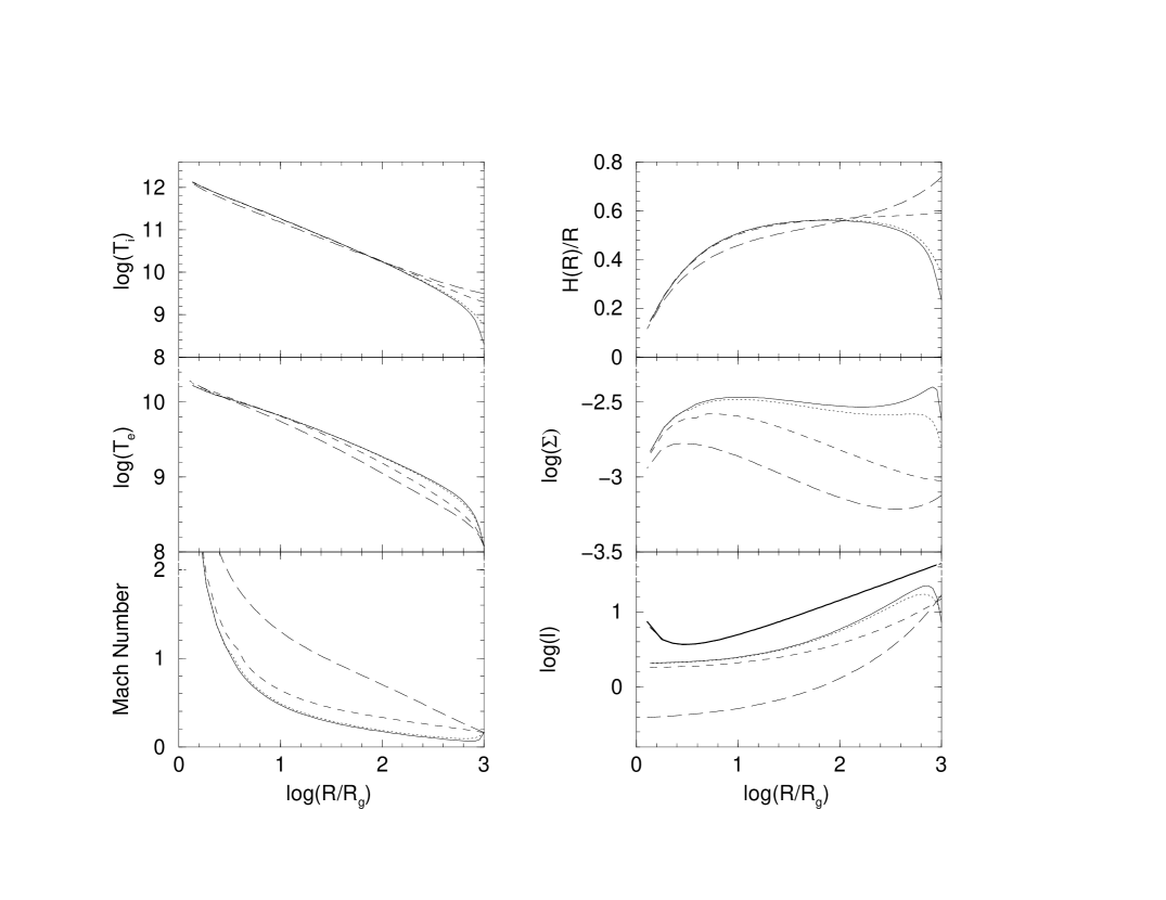
We find that the results are qualitatively the same as in Paper I although the synchrotron radiation, a strong local cooling term, is included in the electron energy equation. This is because the differential terms, which stand for the global character of the equations, still play a dominated role. We find that only when OBCs are within a certain range do the global solutions exist. In terms of the ion temperature, the range is ( here denotes the virial temperature). The electrons temperature is slightly lower than . As for the range of , it must satisfy , otherwise the viscous heating term takes a negative value under our viscous description. This result was first pointed out by Manmoto, Mineshige & Kusunose (1997). The range of OBCs slightly varies under different parameters and , and it is also the function of the value of , as we describe in the subsequent section of this paper. The structures of the solutions with different OBCs are greatly different. Three types of solutions are also found in terms of their topological structures and angular momentum profiles (cf. Paper I). Generally, when is relatively low, the solution is of type I. When is high and is small (or equivalently is large), the solution is of type II. Types I and II both have small values of sonic radii , but their angular momentum profiles are different (see Figure 1 of Paper I and Figure 1 in the present paper). When is high and is large (or equivalently is small), the solution becomes type III, which has much larger .
Figure 1 shows the effect of different on the solution structures. The values of and are the same, with and . The solid line (belonging to type I solution) is for , the dotted line (type I) for , the short-dashed line (type II) for and the long-dashed line (type III) for . Six plots in the figure show the radial variations of the Mach number (defined as so that the Mach number equals 1 at the sonic point), the electrons and ions temperatures, profiles of the specific angular momentum and surface density (), and the ratio of the vertical scale height of the disk to the radius, respectively. From the figure, we find that the discrepancy in the ion temperature is rapidly reduced as the radius decreases and converges to the virial temperature. This is because the local viscous dissipation in the ions energy equation plays an important role therefore the temperature of ions is mainly “locally” determined, like the case of a one-temperature plasma (Paper I). However, the discrepancy in the surface density of the disk persists throughout the disk.
Such discrepancy in the solution structures results in the discrepancy in the emission spectrum, as Figure 2 shows. The discrepancy in the luminosity at certain individual wave band can be understood by referring to Figure 1. In the radio-submillimeter band, the power is principally due to synchrotron emission for which we approximately have for the “general” frequency and for the peak frequency (Mahadevan 1997). Synchrotron radiation mainly comes from the inner region of the disk, . So the long-dashed line in the figure possesses the lowest radio power is mainly due to its lowest surface density, since is almost the same for different solutions. For such a low mass accretion rate system as considered in this paper, the low frequency part of the submillimeter to hard X-ray spectrum is mainly contributed by the Comptonization of synchrotron photons, and it is bremsstrahlung emission that is responsible for the high frequency part. The long-dashed line still possesses the lowest power in the low frequency band because its corresponding amount of synchrotron soft photons is the least and its corresponding Compton y-parameter is the smallest. In the X-ray band, the solid line has the highest power. This is because for bremsstrahlung emission we approximately have , i.e., the density instead of is the dominated factor, and the solid line possesses the highest density among the four solutions.
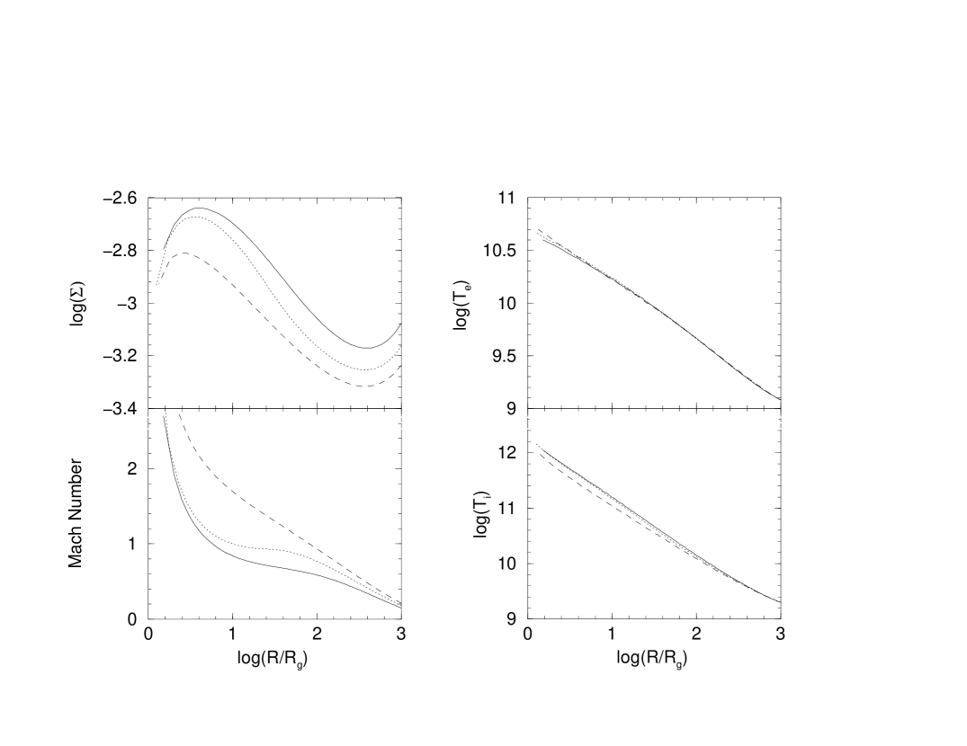
The effect of on the structures of the global solutions is shown in Figure 3. All the three lines in the figure have and . The solid line is for , the dotted line for and the dashed line for . Different with , the discrepancy in persists throughout the disk rather than converges as the radius decreases. This is because the electrons are essentially adiabatic for the present low accretion rate case, i.e., both and are very small compared with the advection term on the left-hand side of equation (8), so the electron temperature is globally determined. While for the ion, the local viscous dissipation in the energy equation plays an important role; thus, the temperature of ion is determined more locally than the electron. Such discrepancy in the electron temperature produces significant discrepancy in the emission spectrum especially in the radio, submillimeter and IR bands, as Figure 4 shows.
The effect of modifying (i.e., modifying ) on the structure of the accretion flows is shown in Figure 5. Each of the three lines in the figure corresponds to and . The values of are (solid line, type II), (dotted line, type II) and (dashed line, type III), and their corresponding angular velocities are and , respectively.
When decreases across a certain critical value, in the present case, an accretion pattern characterized by possessing a much larger sonic radius appears (referred to as type III solution). As we argue later in this paper, this accretion pattern is of particular interest to us. In all previous works on viscous accretion flows, only the solutions with small sonic radii several have been found (Muchotreb & Paczyński 1982; Matsumoto et al. 1984; Abramowicz et al. 1988; Chen & Taam 1993; Narayan, Kato & Honma 1997; Chen, Abramowicz & Lasota 1997; Nakamura et al. 1997); therefore, this pattern is new. The reason why previous authors did not find this pattern is that they generally set the standard thin disk solutions as the OBCs (Muchotreb & Paczyński 1982; Matsumoto et al. 1984; Abramowicz et al. 1988; Chen & Taam 1993; Narayan, Kato & Honma 1997; Chen, Abramowicz & Lasota 1997), where the specific angular momentum of the flow is Keplerian; or, a specific angular momentum with a value near the Keplerian one is set as the OBC (Nakamura et al. 1997; Manmoto, Mineshige & Kusunose 1997).
Such transition between the sonic radii happened when passes across a critical value is clearly shown in Figure 6. The value of the critical varies with the parameters such as and , and it is also the functions of and . Generally, it decreases with the decreasing and/or the increasing . Similar transition has been found previously in the context of adiabatic (inviscid) accretion flow by Abramowicz & Zurek (1981). In that case, they found that when the specific angular momentum of the flow , a constant of motion, decreased across a critical value (here the specific energy of the flow is another constant of motion), a transition from a disk-like accretion pattern to a Bondi-like one would happen (Abramowicz & Zurek 1981; Lu & Abramowicz 1988). Here in this paper we find that this transition still exist when the flow becomes viscous, confirming the prediction of Abramowicz & Zurek (1981).
The physical reason of the transition between the two patterns is obvious. When the specific angular momentum of the gas is low, the centrifugal force can be neglected and the gravitational force plays a dominated role in the radial momentum equation (eq. 6), therefore the gas becomes supersonic far before the horizon like in Bondi accretion. When the specific angular momentum is high, however, since the centrifugal force becomes stronger, the gas becomes transonic only after passing through a sonic point near the horizon with the help of the general relativistic effect (Abramowicz & Zurek 1981; Shapiro & Teukolsky 1984).
Figure 7 shows the corresponding spectra of the solutions presented in Figure 5. The accretion flow belonging to the new accretion pattern, which is denoted by the dashed line, emits the lowest X-ray luminosity. This is because this accretion pattern possesses the largest sonic radius therefore the corresponding density of the accretion flow is the lowest.
All above results are obtained for a fixed outer boundary . We also investigate the influence of increasing the value of on the global solutions. We find that the general feature are quantitatively the same. One remarkable difference is that the ranges of and within which we can obtain a global solution lessen with the increasing radii. For example, if we increase from to , the temperature range will lessen from to . If is taken to be large enough, almost be unique. However, the feasible range of is almost constant, no matter how large is. Moreover, when the value of becomes larger, the transition between the accretion patterns, happened when pass across the critical value, becomes more “obvious” in the sense that the small sonic radius becomes smaller and the large sonic radius becomes larger. Consequently, the discrepancy between the surface density of the accretion disk of the two accretion patterns becomes larger compared with the case of small , and this will further result in the increase of the discrepancy of the X-ray luminosity emitted by the accretion flow. This is the crucial factor to solve the puzzle of the mass accretion rate of Sgr A∗.
4 APPLICATION TO Sgr A∗
Kinematic measurements suggest that the energetic radio source Sgr A∗ located at the center our Galaxy is a supermassive compact object with a mass . This is widely believed to be a black hole (Mezger, Duschl & Zylka 1996). On the other hand, observations of gas outflows near Sgr A∗ indicate the existence of a hypersonic stellar wind coming from the cluster of stars within several arc-seconds from Sgr A∗. The wind should be accreting onto the black hole (Melia 1992). If the flow past Sgr A∗ is uniform, then the mass accretion rate can be simply obtained by the classical Bondi-Hoyle scenario (Bondi & Hoyle 1944) as follows. Since the wind is significantly hypersonic, as such, a standing bow-shock is inevitable. This shock is located roughly where flow elements’ potential energy equals kinetic energy (Shapiro 1973; Melia 1992), , where is the mass of the black hole and is the wind velocity. From here the shocked gas is assumed to accret into the hole. Since the mass flux in the gas at large radii is , where is proton mass and is the number density of the gas, the mass accretion rate is .
This result is only valid for an uniform source. In reality the flow past Sgr A∗ comes from multiple sources. In this case, the wind-wind shocks dissipate some of the bulk kinetic energy and lead to a higher capture rate for the gas (Coker & Melia 1997). The exact value of accretion rate depends on the stellar spatial distribution and can only be obtained by numerical simulation. The three-dimensional hydrodynamical simulation of Coker & Melia (1997) gives the average value for two extreme spatial distributions, spherical and planar ones. With the available data at that time, the accretion rate obtained in Coker & Melia (1997) is . Considering that recent work suggests the Galactic Centre wind is dominated by a few hot stars with higher wind velocities of (Najarro et al. 1997) rather than taken by Coker & Melia (1997), the more reliable accretion rate should be .
Assuming the accretion is via a standard thin disk, the accretion rate required to model the luminosity is more than three orders of magnitude lower than this value. ADAF model has been turned out to be a significant success to model its low luminosity (Narayan, Yi & Mahadevan 1995; Manmoto, Mineshige & Kusunose 1997; Narayan et al. 1998). However, there exists a discrepancy between the accretion rate favored by all ADAF models in the literature and that favored by the simulation mentioned above, with the former being 10-20 times smaller than that favored by the latter (Coker & Melia 1997; Quataert & Narayan 1999b). The most up-to-date calculation gives (Quataert & Narayan 1999b) and this value approaches the lower limit considered plausible from Bondi capture (Quataert, Narayan, & Reid 1999). In an ADAF model, the mass accretion rate is determined by fitting the theoretical X-ray flux to the observation. If a larger accretion rate were adopted, then bremsstrahlung radiation would yield an X-ray flux well above the observational limits. Even though we assume that significant accretion mass may be lost to a wind, detailed calculation shows that since the bremsstrahlung radiation comes from large radii in the accretion flow, the discrepancy can not be alleviated no matter how strong the winds are (Quataert & Narayan 1999b).
The present research on the role of OBC tells us that we should seriously consider the physical state of accretion flows at the outer boundary. However, we note that in all present ADAF models of Sgr A∗, the outer boundary condition is roughly treated. In our view, this might be an origin of the discrepancy between the mass accretion rate.
Basing upon the above consideration, we recalculate the spectrum of Sgr A∗. We set the outer boundary at the “accretion radius” . In the present case of Sgr A∗, the temperatures of ions and electrons in the flow just after the bow-shock should equal the virial temperature . But the value of the specific angular momentum at the outer boundary is not certain. We set it as various values and find that, when it pass across a critical value , the transition of the accretion pattern occurs. Figure 8 shows the Mach number and the surface density of the two accretion patterns. The parameters of both the solid and the dashed lines in the figure are: , , and . At the outer boundary , the two lines possess identical temperature of , but their specific angular momenta are different. The solid line, which stands for our new accretion pattern, corresponds to relatively low angular velocity, , while the angular velocity possessed by the dashed line, which we draw for comparison, is much higher, . Their sonic radii are (dashed line), and (solid line), respectively. The difference of the sonic radius results in the discrepancy in the surface density, which further results in the difference of the X-ray luminosity, as shown by Figure 9.
Figure 9 shows our calculated X-ray spectra together with the observation of Sgr A∗. Here we assume that the bremsstrahlung radiation is the only contributor to this waveband. This assumption requires that the synchrotron radiation can not be too strong, otherwise the contribution from the Comptonization of the synchrotron photons will exceed that from bremsstrahlung radiation. This requirement can be satisfied according to the radio observation of Sgr A∗. We will discuss this question in the following part. From the figure, we find that accretion rate as high as is acceptable, if only the angular momentum at the outer boundary is relatively low. Compared with the value of in Quataert & Narayan (1999b), this value is much closer to that favored by the numerical simulation. If the angular momentum of the flow at is relatively high, however, as shown by the dashed line, the X-ray flux is well above the observation.
Now the crucial moment is whether the value of the angular velocity at is really low. In this context, we note that the three-dimensional numerical simulation by Coker & Melia (1997) indicates that the accreted angular velocity in Sgr A∗ is very low, for their run 1 and for their run 2. The consistency with our result is satisfactory.
5 SUMMARY AND DISCUSSION
In this paper, we numerically solve the radiation hydrodynamic equations describing an optically thin advection dominated accretion flow and calculate its emergent spectrum. We fix all the parameters such as and , and set the outer boundary condition as and at certain outer boundary . Our primary focus is to investigate the effects of the outer boundary conditions on the structure of the global solution and, especially, on the emergent spectrum.
We find that OBCs must lie in a certain range, otherwise we can’t find the corresponding global solutions. However, this range is large enough in the sense that both the structure of the solution and its corresponding spectrum differ greatly from each other under different OBCs. Three types of solutions are also found under various OBCs, qualitatively agree with the result of Paper I, where magnetic field is neglected and the description to radiation is crude. The value of the sonic radius in type III solution is much larger than types I and II. We examine the individual influence of and on the structures and spectrum and find that each factor especially the temperature, plays a significant role. The peak flux in the radio, IR and X-ray bands can differ by nearly two orders of magnitude or more in our example, although all the other parameters are exactly the same.
We also investigate the effect of modifying the value of . We find that the feasible ranges of and lessen with the increasing radii. If the value of is too large, the values of and are almost unique. This result seems to mean the reduction of the effect of OBC on the solution. However, on the one hand we expect that in some cases, such as some binary system or the system where a thin disk-ADAF transition is expected to occur (e.g., X-ray binaries A0620-00 and V404 Cyg, and low luminosity AGN NGC 4258; see Narayan, Mahadevan, & Quataert 1998 and references therein), the value of might be small. On the other hand, the feasible range of is almost constant no matter how large is.
The reason why previous works on ADAF global solution (e.g., Narayan, Kato, & Honma 1997; Chen, Abramowicz, & Lasota 1997) did not find the obvious effect of OBC on the global solution is that, both Narayan, Kato & Honma (1997) and Chen, Abramowicz & Lasota (1997) concentrated on the dynamics of a one-temperature plasma, where the local viscous dissipation in the energy equation plays an important role. Due to this reason, their global solutions are in principle “locally” rather than “globally” determined, the effect of OBC weakens rapidly with the decreasing radii and the solutions converged rapidly over a small radial extent away from the outer boundary. We also obtained similar results with theirs for the one-temperature plasma in our Paper I. However, according to our result, the variation of across a certain critical value will produce obvious OBC-dependent behavior such as the transition of the sonic radius, no matter what type the plasma is, one- or two-temperature. They did not find this result might be due to the fact that adopted by them, for Keplerian disk outer boundary condition or for self-similar solution outer boundary condition, is always larger than the critical value, so the effect of OBC is very small hence is hard to find.
The present study concentrates on the low- case where the differential terms in the equation such as the energy advection play an important role therefore the effect of OBC are most obvious. When becomes higher, the role of the local radiation loss terms in the energy balance will become more important. In this case, we expect that the discrepancy due to OBC in the profile of the temperature will lessen. However, from our calculation to the one-temperature accretion flow whose temperature is also principally determined locally (Paper I), and Figure 5 in the present paper, we expect that the flow should still present OBC-dependent behavior in, e.g., the angular momentum and the Mach number profiles.
We do not include winds in the present study. Since the Bernoulli parameter of ADAF is positive therefore the gas can in principle escape to infinity with positive energy (Narayan & Yi 1994, 1995). Blandford & Begelman (1999) recently suggested that mass loss through winds might be dynamically important. The effect of winds on the spectrum of ADAF has been investigated by Quataert & Narayan (1999b). It is interesting to investigate the effect of OBC on ADAF with winds. We expect the result is probably similar with the present results since in that case the differential terms in the equation still play an important role.
It is a meaningful problem whether a standing shock occurs in an accretion flow. Although some authors have set up the shock-included global solutions (e.g. Chakrabarti 1996), the result is generally thought not to be so convincing because in their numerical procedure and are treated as two free parameters instead of the eigenvalues of the problem. A necessary condition for the shock formation is the existence of the global solution with a large sonic radius outside the centrifugal barrier. This is the key of the problem. According to our result, this kind of large-sonic-radius solution, belonging to our type III, can only be realized when the specific angular momentum of the accretion flow is low. We note that this requirement to the angular momentum is exactly what Narayan, Kato & Honma(1997) anticipated, and it has recently been confirmed by the numerical simulation by Igumenshchev, Illarionov & Abramowicz (1999).
The large-sonic radius solution (type III) is a new accretion pattern since in all previous studies on viscous accretion onto black holes the sonic radii are small. We find that the discrepancy in the mass accretion rate of Sgr A∗ between the value favored by the previous ADAF models in the literature and that favored by the hydrodynamical numerical simulation is significantly reduced if the accretion is via this pattern. This result hints us that such low angular momentum accretion may be very common in the universe. One example is the detached binary system, where the accretion material is the stellar wind from the companion therefore the angular momentum of the accreting gas is very low (Illarionov & Sunyaev 1975). Another example is the cores of nearby giant elliptical galaxies, where the angular momentum of the hot (accretion) gas is again assumed to be very small.
Acknowledgements.
We are grateful to the referee for many helpful comments and suggestions which enabled us to improve the presentation. This work is supported in part by the National Natural Science Foundation of China under grant 19873007. F.Y. also thanks the financial support from China Postdoctoral Science Foundation.References
- (1) Abramowicz, M.A., Chen, X., Kato, S., Lasota, J.-P., & Regev, O. 1995, ApJ, 438, L37
- (2) Abramowicz, M.A., Czerny, B., Lasota, J.P., & Szuszkiewicz, E., 1988, ApJ, 332, 646
- (3) Abramowicz, M., A., Zurek, W.H., 1981, ApJ, 246, 31
- (4) Begelman, M.C., 1978, MNRAS, 243, 610
- (5) Begelman, M.C., & Meier, D.L., 1982, ApJ, 253, 873
- (6) Blandford, R.D., & Begelman, M.C. 1999, MNRAS, 303, L1
- (7) Bondi, H. & Hoyle, E. 1944, MNRAS, 104, 273
- (8) Chakrabarti, S.K. 1996, ApJ, 464, 664
- (9) Chandrasekhar, S. 1939, Introduction to the Study of Stellar Structure(New York: Dover)
- (10) Chen, X., Abramowicz, M. A., & Lasota, J.-P. 1997, ApJ, 476, 61
- (11) Chen, X. & Taam, R. 1993, ApJ, 412, 254
- (12) Coker, R., & Melia, F., 1997, ApJ, 488, L149
- (13) Coppi, P.S., & Blandford, R.D. 1990, MNRAS, 245, 453
- (14) Dermer, C.D., Liang, E.P., & Canfield, E. 1991, ApJ, 369, 410
- (15) Esin, A.A., Narayan, R., Ostriker, E., & Yi, I. 1996, ApJ, 465, 312
- (16) Esin, A.A., 1997a, ApJ, 482, 400
- (17) Esin, A.A., McClintock, J. E., & Narayan, R. 1997b, ApJ, 489, 865
- (18) Ichimaru, S., 1977, ApJ, 214, 840
- (19) Igumenshchev, I.V., Illarionov, A.F. & Abramowicz, M.A. 1999, ApJ, 517, L55
- (20) Illarionov, A.F., & Sunyaev, R.A., 1975, A&A, 39, 185
- (21) Lu, J.F., & Abramowicz, M.A. 1988, Acta Ap. Sin., 8, 1
- (22) Mahadevan, R. 1997, ApJ, 477, 585
- (23) Manmoto, T., Mineshige, S., Kusunose, M. 1997, ApJ, 489, 791
- (24) Matsumoto, R., Kato, S., Fukue, J., & Okazaki, A.T. 1984, PASJ, 36, 71
- (25) Melia, F 1992, ApJ, 1992, 387, L25
- (26) Mezger, P.G., Duschl, W.J., & Zylka, R. 1996, A&AR, 7, 289
- (27) Muchotreb, B., & Paczyński, B. 1982, Acta Astron. 32, 1
- (28) Najarro, E., et al. 1997, A&A, 325, 700
- (29) Nakamura, K. E., Kusunose, M., Matsumoto, R., & Kato, S. 1997, PASJ, 49, 503
- (30) Narayan, R., Kato, S. & Honma, F. 1997, ApJ, 476, 49
- (31) Narayan, R., Mahadevan, R., Grindlay, J.E., Popham, R. & Gammie, C., 1998, ApJ, 492, 554
- (32) Narayan, R., Mahadevan, R., & Quataert, E. 1998, in “The Theory of Black Hole Accretion Discs”, eds. M.A. Abramowicz, G. Bjornsson, and J.E. Pringle, (Cambridge University Press)
- (33) Narayan, R. & Yi, I. 1994, ApJ, 428, L13
- (34) Narayan, R. & Yi, I. 1995, ApJ, 444, 231
- (35) Narayan, R., Yi, I., Mahadevan, R. 1995, Nature, 374, 623
- (36) Paczyński, B., & Wiita, P. J. 1980, A&A, 88, 23
- (37) Quataert, E., & Narayan, R., 1999a, ApJ, 516, 399
- (38) Quataert, E., & Narayan, R., 1999b, ApJ, 520, 298
- (39) Quataert, E., Narayan, R., & Reid, M.J. 1999, ApJ, 517, L101
- (40) Rybicki, G., & Lightman, A.P. 1979, Radiative Processes in Astrophysics (New York: Wiley)
- (41) Rees, M.J., Begelman, M.C., Blandford, R.D., & Phinney, E.S., 1982, Nature, 295, 17
- (42) Shakura, N.I., & Sunyaev, R.A., 1973, A&A, 24, 337
- (43) Shapiro, S.L. 1973, ApJ, 180, 531
- (44) Shapiro, S.L., & Teukolsky, S.A. 1984, Black Holes, White Dwarfs, and Neutron Stars (New York: Wiley)
- (45) Yuan, F. 1999, ApJ, 521, L55 (Paper I)
- (46)
- (47)
- (48)