The Warp of the Galaxy and the Orientation of the LMC Orbit

Abstract

After studying the orientation of a warp generated by a companion satellite, we show that the Galactic Warp would be oriented in a different way if the Magellanic Clouds were its cause. We have treated the problem analytically, and complemented it with numerical N-Body simulations.

1 Introduction

The disk of the Milky Way is remarkably flat out to 10 kpc, where it starts to bends in opposite directions in the southern and northern parts. The cause of it is still a puzzle: for a review, see Binney [Binney 1992].

One possibility is that the Magellanic Clouds distort the Galactic disk in the observed way. The fact that the direction of the maximum warping lies very close to the galactocentric longitude of the Clouds makes this hypothesis tempting.

The problem with this scenario is that the Clouds are not massive enough to generate the warp amplitudes that we observe at their present distance. This was noticed by the first researches in this field [Burke 1957, Kerr 1957], and later by Hunter & Toomre (1969). A remedy which might allow this scenario to work was to suppose that the Clouds are currently not at the pericenter of their orbit, so that they have been much closer to the Galactic disk in a previous epoch ($\simeq 20$ kpc is what was needed). However, later work by Murai & Fujimoto (1986) determined the orbit of the Clouds, and proved that the Clouds are actually at their pericenter, with an apocenter close to 100 kpc, so the problem of the small amplitude still remains if the Clouds are to be blamed as the cause of the Galactic warp.

Recently a mechanism for amplifying the effect of a satellite has been proposed by Weinberg [Weinberg 1998]. He describes a calculation in which a disk galaxy surrounded by a dark halo is perturbed by a massive satellite, similar to the LMC. By means of a linear perturbation analysis, he follows the perturbation (wake) created by the satellite in the halo, including its self-gravity. He finds that the torque exerted on the disk is several times larger than that due directly to the satellite: the latter is amplified because (i) the satellite-induced wake in the halo itself exerts a torque, roughly in phase with that from the satellite; and (ii) the wake itself further perturbs the halo, resulting in a torque that is larger again. Under circumstances in which the satellite orbital frequency is close to the natural precession frequency of the disk (i.e., the warp mode frequency of Sparke & Casertano [Sparke & Casertano 1988]), a significant amplitude can result. A calculation by Lynden-Bell [Lynden-Bell 1985] of a similar scenario gives comparable results, as does a simple model described by Kuijken [Kuijken 1997].

In this paper, we focus on the orientation of a warp generated by a massive orbiting satellite with less emphasis on the amplitude of the warp. In §2 we discuss a simple analytic model in which the disk and halo are rigid: this establishes the baseline response of a disk to satellite tides, and its orientation with respect to the satellite orbital plane. As we show, this orientation is different from that of the Galactic warp to the LMC orbit. §3 contains a description of the N-body code used, and §4 to §6 the results of our N-body simulations, showing that the orientation problem remains. In §7 we give our conclusions.

2 Analytic results with a simplified model

A simple model serves as a reference for the warp response of the disk to an orbiting satellite. Consider a rigid disk, embedded in a rigid halo potential, and subjected to the potential of an orbiting satellite. The evolution of the disk is governed by the combined torque from halo and satellite. A stellar or gaseous disk is floppy, and so will warp when tilted, since it is not able to generate the stresses that would be required to keep it flat; however the overall re-alignment of the disk angular momentum should be comparable between the rigid and floppy cases.

The angles used in this paper related to the satellite, and the definition of our coordinate system are illustrated in Figure 1. The tilting of the disk is measured by the angle between the $z$ axis and the angular momentum of the disk. The longitude of this vector is the same as the longitude of the maximum of the warp when looking at the disk from the North Galactic Pole.

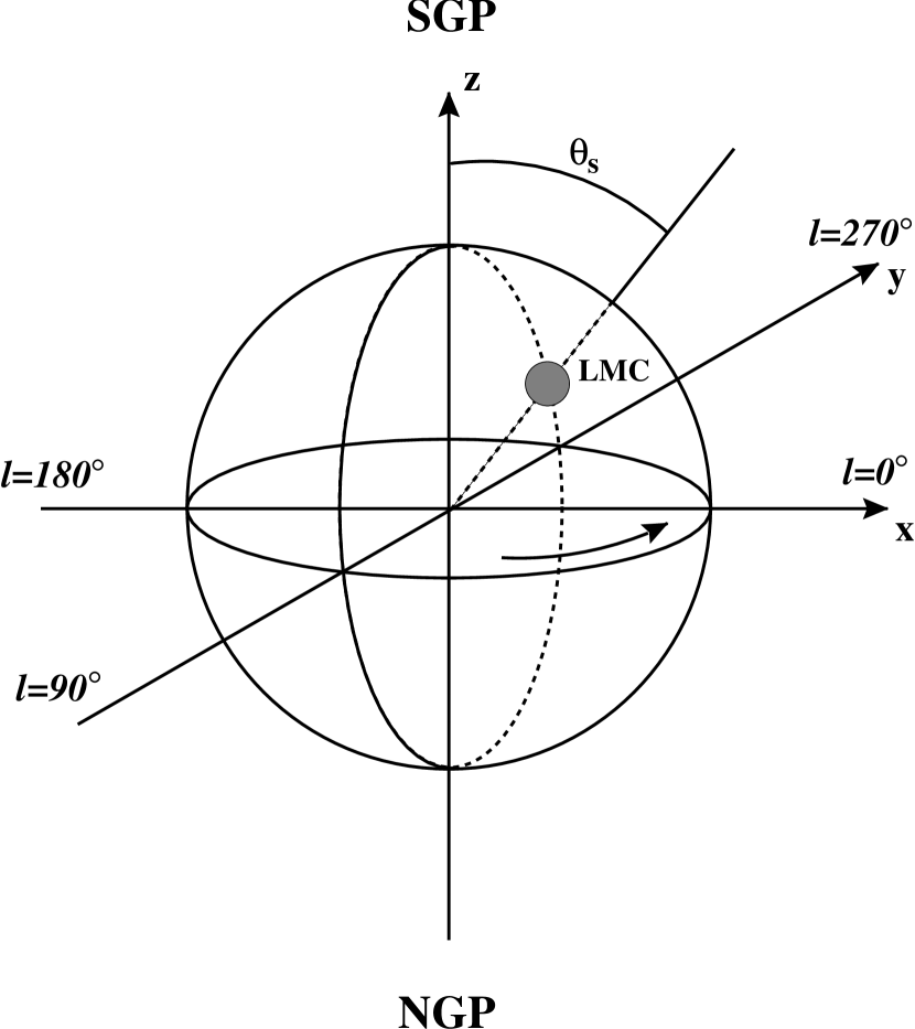
Figure 1: Definition of the coordinate system, satellite angles, and orientation of the disk of the Galaxy. The disk lies on the $z=0$ plane. The sun is on the left, and the galactic plane is viewed from the South Galactic Pole so that the disk rotates counterclockwise (indicated by an arrow).

The Lagrangian for a rigidly spinning, axisymmetric object is

$${\cal L}=\textstyle{\frac{1}{2}}I_{1}(\dot{\theta}^{2}+\dot{\phi}^{2}\sin^{2}\theta)+\textstyle{\frac{1}{2}}I_{3}(\dot{\phi}\cos\theta+\dot{\psi})^{2}-V(\theta,\phi)$$ (1)

where $(\theta,\phi,\psi)$ are the Euler angles, and $I_{3}$ and $I_{1}$ are the moments of inertia of the object about its symmetry axis and about orthogonal directions. $V$ is the potential energy of the body in the halo plus satellite potential. The $\psi$-equation of motion leads to the conserved quantity $S=I_{3}(\dot{\phi}\cos\theta+\dot{\psi})$, the spin, and the other two equations of motion then become

$$I_{1}\ddot{\theta}-I_{1}\dot{\phi}^{2}\sin\theta\cos\theta+S\dot{\phi}\sin\theta+{\partial V\over\partial\theta}=0$$ (2)

and

$$I_{1}{{\mathrm{d}}\over{\mathrm{d}}t}({\dot{\phi}\sin^{2}\theta})+{\partial V\over\partial\phi}=0.$$ (3)

For small deviations from the equator ($\theta=0$), we can expand these equations in terms of $x=\sin\theta\cos\phi\simeq\theta\cos\phi$, $y=\sin\theta\sin\phi\simeq\theta\sin\phi$. In these terms the equations of motion become

$$I_{1}\ddot{x}+S\dot{y}+{\partial V\over\partial x}=0,$$ (4)

$$I_{1}\ddot{y}-S\dot{x}+{\partial V\over\partial y}=0.$$ (5)

For small $x,y$, the potential energy of the disk due to the flattened halo will have the form $\textstyle{\frac{1}{2}}V_{\mathrm{H}}(x^{2}+y^{2})$, and that due to the satellite at position $\theta_{\mathrm{S}},\phi_{\mathrm{S}}$ will be $-V_{\mathrm{S}}(\sin^{2}\theta_{\mathrm{S}}-x\sin 2\theta_{\mathrm{S}}\cos\phi_{\mathrm{S}}-y\sin 2\theta_{\mathrm{S}}\sin\phi_{\mathrm{S}})$ where $V_{\mathrm{H}}$ and $V_{\mathrm{S}}$ are constants representing the strengths of the halo torque and of the quadrupole of the tidal field from the satellite, respectively. Hence we find

$$I_{1}\ddot{x}+S\dot{y}+V_{\mathrm{H}}x+V_{\mathrm{S}}\sin 2\theta_{\mathrm{S}}\cos\phi_{\mathrm{S}}=0,$$ (6)

$$I_{1}\ddot{y}-S\dot{x}+V_{\mathrm{H}}y+V_{\mathrm{S}}\sin 2\theta_{\mathrm{S}}\sin\phi_{\mathrm{S}}=0.$$ (7)

If furthermore the satellite orbit is circular and polar in the $x=0$ plane, $\theta_{\mathrm{S}}=\Omega_{\mathrm{S}}t$, $\phi_{\mathrm{S}}=90$, and the solution to the equations of motion is

$$x={2\Omega_{\mathrm{S}}S\over\Delta}V_{\mathrm{S}}\cos 2\Omega_{\mathrm{S}}t;\quad y={4I_{1}\Omega_{\mathrm{S}}^{2}-V_{\mathrm{H}}\over\Delta}V_{\mathrm{S}}\sin 2\Omega_{\mathrm{S}}t$$ (8)

plus free precession and nutation terms, where $\Delta=(V_{\mathrm{H}}-4I_{1}\Omega_{\mathrm{S}}^{2})^{2}-4\Omega_{\mathrm{S}}^{2}S^{2}$. (A more general quasiperiodic satellite orbit yields a solution which can be written as a sum of such terms.) Notice that the satellite provokes an elliptical precession about the halo symmetry axis, with axis ratio dependent on the halo flattening and on the satellite orbit frequency. For example, for an exponential disk of mass $M$, scale length $h$ and with a flat rotation curve of amplitude $v$, $I_{3}=2I_{1}=6Mh^{2}$ and $S=2hvM$. For such a disk in a spherical (or absent) halo ($V_{\mathrm{H}}=0$), a satellite orbiting at radius $r_{\mathrm{S}}$ has frequency $\Omega_{\mathrm{S}}=v/r$, and hence the axis ratio of the forced precession is $(x:y)=r_{\mathrm{S}}/3h$. Hence the response of the disk to a distant satellite is mainly to nod perpendicular to the satellite orbit plane. This result can be understood as the classic orthogonal response of a gyroscope to an external torque: a distant satellite has a sufficiently low orbital frequency that the disk responds as if the torque were static.

For a slightly flattened potential of the form $\textstyle{\frac{1}{2}}v^{2}\ln[R^{2}+(z/(1-\epsilon))^{2}]$, $V_{\mathrm{H}}=Mv^{2}\epsilon$. With non-zero $\epsilon$, the axis ratio of the precession cone becomes $[(4h/r_{\mathrm{S}})/(\epsilon-12h^{2}/r_{\mathrm{S}}^{2})]$: again the oscillation in $x$ is larger than that in $y$ except for very flattened halos.

The amplitudes generated by tidal perturbation from a satellite such as the LMC are small, less than a degree. The largest amplitude of oscillation is in the $y$-direction. The potential energy of the disk due to the tidal field of the satellite can be shown to be (see Appendix)

$$V_{\mathrm{S}}={3GM_{\mathrm{S}}I_{1}\over 2r_{\mathrm{S}}^{3}}.$$ (9)

Hence equation 8 yields, to leading order in $h/r_{\mathrm{S}}$, an $x$-amplitude of

$$\frac{9}{8}\frac{GM_{\mathrm{S}}}{v^{2}r_{\mathrm{S}}}\frac{h}{r_{\mathrm{S}}}\simeq 0.09^{\circ}$$ (10)

for the LMC (orbital radius about $50\,\mathrm{k}pc$, and $r_{\mathrm{S}}/h\simeq 15$). This number increases only slightly (a factor 2) for halo flattenings up to 0.2 (see Figure 2).

Figure 2: The oscillation of the axis of a rigid exponential disk subjected to the tidal field of an orbiting satellite. The amplitude is calculated assuming a satellite of mass $1.5\times 10^{10}M_{\odot}$, orbiting at radius $54\mathrm{k}pc$ in the $z=0$ plane. The direction of the tilt of the Galactic disk with respect to the Magellanic Clouds’ orbital plane is indicated by the arrow. The dots mark the expected position of the disk axis given the current phase of the LMC orbit for (bottom to top) halo potential ellipticities $\epsilon=0$ (solid symbol),$0.05,0.1,0.15$ and 0.2 (open circles).

It is clear from this calculation that simple tidal tilting of a disk by an LMC-like satellite does not provide a good model for the warping in the Galaxy, because the orientation of the warp is not perpendicular to the orbital plane of the LMC. This constraint is independent of the strength of the perturbation $V_{\mathrm{S}}$.

The amplitudes are much too small, but we have only considered the tilting of a rigid disk, and the situation can change when the floppiness of the disk is considered.

3 Simulation details

To test this scenario, and in particular to get beyond the rigid tilting considered above, we have performed some N-body simulations. We assume the halo to be a background potential which does not respond to the disk or the satellite.

The N-body code used for this work models the disk as a set of concentric spinning rings embedded in a spherical, rigid halo. This description allows warps to be described, but not in-plane distortions of the disk such as bars or lopsidedness.

3.1 Initial conditions

We have performed simulations with two types of disks: a rigid disk and a exponential disk. The rigid disk run tells us how good the analytic predictions are, and the exponential disk is used later for a more realistic approach.

We use a King model for the halo, in order to obtain a reasonable flat rotation curve (Figure 3). This is accomplished with a model of $\Psi_{0}/{{\sigma}_{0}}^{2}=-6$, a tidal radius of 44 (200 kpc. for a 4.5 kpc scale-length disk), and mass of 10 disk masses.

Each of the disks is made of 1000 rings, each of them consisting of 36 particles. Various runs where made with more rings and more particles per ring, without important changes in the results described below.

Figure 3: Rotation curve showing the contribution from the disk (dotted) and halo (dashed) to the total (solid)

The satellite is modelled as having a Plummer distribution. To avoid relative movements of the galaxy with respect to the satellite we have used two satellites instead of one, symmetrically placed with respect to the centre of the halo-disk system. This causes the dipole term of the tidal field to be zero, avoiding relative movements of the galaxy with respect to the satellites. It is equivalent to only keeping the even-$l$ terms in the potential of the satellite, neglecting the dipole, $l=1$, terms in the potential, and concentrating on the warp (which result from the quadrupole, $l=2$ terms).

The first run was made with a satellite in a circular orbit, to try to reproduce the predictions in §2. Later a non-circular orbit is considered, and the difference between both simulations analysed. The non-circular orbit has a pericenter at 50 kpc and apocenter at 100 kpc, consistent with recent determination of the orbit of the Clouds [Lin, Jones & Klemola 1995]. In the non-circular simulations the satellite starts at its apocenter at the beginning of the simulation, where the perturbation on the disk is the smallest possible.

The units of the model translate to the Galaxy (disk scale-length $4.5\,\mathrm{k}pc$, and the rotation velocity at $8.5\,\mathrm{k}pc$ of $220\,\mathrm{k}m\,s^{-1}$) as follows: length unit = $4.5\,\mathrm{k}pc$, velocity unit = 340 $\mathrm{k}m\,s^{-1}$, time unit = $1.30\times 10^{7}\,$years, mass unit= $1.20\times 10^{11}\mathrm{M}_{\odot}$. With these numbers, the disk mass of our model is $6.1\times 10^{10}\mathrm{\,}M_{\odot}$, and the satellite (LMC) has a mass of $1.5\times 10^{10}\mathrm{\,}M_{\odot}$, the biggest current mass estimate for the Clouds [Schommer et al. 1992]. In the coordinate system of the simulations, the $z=0$ is the disk plane, and the orbit of the satellite lies in the $x=0$ plane.

3.2 Code used to evolve the system

The disk is modelled as a system of pivoted spinning rings, fixed at the centre of the halo. Each ring is realized as 36 azimuthally-spaced particles, and the potential generated by the rings is calculated with a tree code [Barnes & Hut 1986]. The forces on the individual “ring-particles” are used to calculate the torque on each ring. The force exerted by a satellite on the ring particles was evaluated directly using the Plummer law.

The Euler equations for rings and axisymmetric bodies can be rewritten in a form so that the time derivatives of the instantaneous angular velocities about the body axes are linear combinations of the angular velocities, torques and body normal vector components. This allows the derivation of a second order explicit time-centred leapfrog integration scheme that can be used to solve the coupled equations for the rings and make it easy to merge with an N-body code [Dubinski 2000].

4 Rigid Disk

As a first approach, we have evolved a rigid disk and analysed its evolution under the influence of an orbiting satellite. The result of our simulation is in good agreement with the analytic predictions. The disk wobbles under the influence of the satellite, describing an ellipse elongated in the direction perpendicular to the satellite’s orbital plane. The path followed by the disk is plotted in Figure 4, where it can be seen that most of the time the maximum of the warp is located in the direction perpendicular to the orbital plane of the satellite ($l=0^{\circ}$ and $l=180^{\circ}$). The ellipse isn’t as regular as in Figure 2 for two reasons: the assumption that the disk is much smaller than the orbital radius of the satellite is not completely fulfilled; and there are some transient terms present because of the initial conditions of the simulation. This are also the cause for the precession ellipse of the disk not to be centred in the origin.

The position of the warp when the satellite is at the location of the LMC is indicated by the dots in Figure 4, and the location of them resembles the predicted one in Figure 2 (for $\epsilon_{halo}=0$) remarkably well.

Figure 4: Precession path followed by the rigid disk: $x=\theta\cos\phi$, $y=\theta\sin\phi$. The dots indicate the disk’s state when the satellite has the LMC’s orbital phase.

5 Exponential self-gravitating Disk

We now consider a more realistic disk: an exponential disk model, in which we have considered also the disk’s self-gravity. The first thing that draws our attention in this simulation is a peak we see in the inclination at around 6.5 scale-lengths. Simulations done with a different rotation curve showed that this peak occurs at the locations on the disk that satisfy $\Omega_{s}/w_{z}=2,3,...$, that are caused by resonances with the satellite’s orbital frequency. This happens because the non-linear behaviour of the outer parts of the disk, where the assumption $r_{s}\gg r_{disk}$ is worse than it is further in.

This is not the kind of warp we are looking for, due to the fact that it is the result of a satellite with a single frequency, and in the real case the eccentric orbit of the satellite will wash out this peak. Looking at the evolution of the disk it is clear that the warp looses its coherence at a radius about 4.5 scale-lengths (at larger radius the line of nodes winds up), so we will measure the warp properties considering that the disk finishes there.

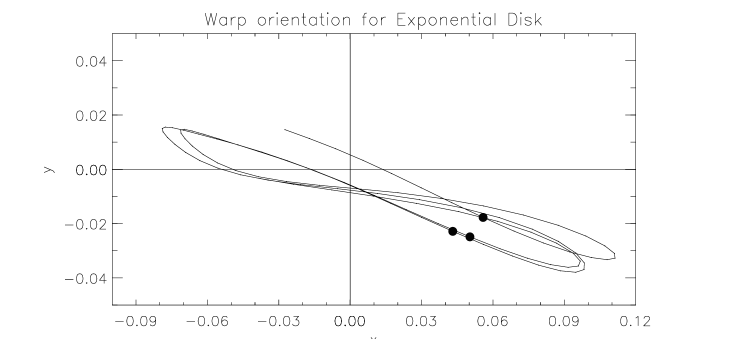
Figure 5: Warp orientation followed by the Exponential Disk: $x=\theta\cos\phi$, $y=\theta\sin\phi$. The dots indicate the disk’s state when the satellite has the LMC’s orbital phase.

In the case of a floppy disk it is not straight-forward to define a single inclination and position angle. We have separated the disk into two components: the inner disk and the outer (warped) disk. The inner disk consists on the first 2 scale-lengths, and remains practically flat along the simulation. The warping angle is then calculated as the angle between the inner and outer disk vectors. We have chosen to use the disk vectors and not the angular momentum, for example, not to penalise the outer less massive rings. The results presented here do not change significantly when the definition of the inner disk is altered.

It has to be kept in mind that the warping angles quoted here are different than the maximum amplitude of the warp, who usually are larger by a factor not greater than 5.

Using this method we obtain a plot similar to Figure 4 for the exponential disk, which is shown in Figure 5. Only the path after t=160 is shown, that is the moment when the disk behaviour reaches an equilibrium.

Note that the predictions for the Galactic Warp don’t really change with the floppiness of the disk: it is clearly close to $l=0^{\circ}$, as chapter §2 predicted, and not at $l=\simeq 90^{\circ}$, as we observe it in the Galaxy.

6 Non-circular orbit, and flattened halos

We also considered non-circular orbits, to allow for the fact that the orbit derived for the Clouds has a pericenter of 50 kpc and an apocenter of 100 kpc [Murai & Fujimoto 1980]. The changing radius of the satellite causes a fluctuating tidal field amplitude, which could be important for the dynamics of the disk. Here we show that in fact the effect does not change our conclusions materially.

First, to have an idea of what to expect, we integrated the analytic equations of section §2 with a satellite in this kind of orbit. The result was, as before, that the disk’s precession path was contained within an ellipse, elongated along the direction perpendicular to the satellite’s plane. This causes the warp maxima to be most of the time close to the direction perpendicular to the satellite’s orbit.

We then performed simulations with this type of orbits. The first thing we observe in these simulations is that the resonance peak we found in the circular orbit simulation has disappeared. Now the satellite doesn’t have a single frequency, so the result is not surprising. The energy of the resonance gets distributed along different parts of the disk now, and no coherent pattern can be maintained across the disk, winding up the outer parts of the disk. When we look at the inner 4.5 scale-lengths as before, the precession pattern remains similar to the simulation with the circular orbit, so does the prediction of the warp’s longitude at LMC’s actual orbital phase. So our conclusions are not modified by the non-circularity of the orbit.

The halos considered in all these simulations are spherical, which means that they don’t contribute to the generation of torques on the disk. We know that halos are not spherical, which creates a preferred plane in which the disk settles. Ellipticities of the order of 0.05 in the potential make the precession paths described before yet more elongated, which would make the chances of finding the warp maxima in the satellites’ direction even more unlikely.

7 Conclusion

We show by means of analytic work and N-body simulations that the precession path of a warp generate by an orbiting satellite galaxy is elongated along the direction perpendicular to the satellite’s orbital plane. Applying our result to the Milky Way, if the Galactic Warp is generated by the Magellanic Clouds, the direction of maximum amplitude of the warp would lie close to $l\simeq 0^{\circ}$, as compared to the observed direction of $\simeq 90^{\circ}$. Even if the halo’s self-gravitating tidal response to the satellite amplifies the effect of the satellite [Weinberg 1998], this response will be mostly in phase with the satellite, and the alignment problems will persist. Possibly the Sagittarius dwarf galaxy, whose orbit lies at 90^∘ to that of the LMC, can be the cause of the warp instead [Ibata & Razoumov 1998].

A limitation of the present work is that the halo has not been considered as a live, self-gravitating component. It has been shown [Dubinski & Kuijken 1995, Nelson & Tremaine 1995] that the back-reaction of the halo on a re-aligning disk can have important consequences. Such effects will be the subject of a further paper.

Appendix A Potential of axisymmetric disk due to a satellite

The potential energy of an disk of surface density $\Sigma(r)$ and in the gravitational field due to a satellite at position ${\mn@boldsymbol{r}}_{\mathrm{S}}$ is given by

$$V=-\int{\mathrm{d}}^{2}{\mn@boldsymbol{r}}\,G\Sigma(r){M_{\mathrm{S}}\over|{\mn@boldsymbol{r}}-{\mn@boldsymbol{r}}_{\mathrm{S}}|}.$$ (11)

Choosing spherical coordinates for the satellite’s position (see Figure 1), and Cartesian coordinates in the disk plane so that the satellite has $x=0$, we have

$$V=-GM_{\mathrm{S}}\int\Sigma{\mathrm{d}}x\,{\mathrm{d}}y\,(r_{\mathrm{S}}^{2}-2yr_{\mathrm{S}}\sin\theta_{\mathrm{S}}+x^{2}+y^{2})^{-1/2}.$$ (12)

Assuming that the disk is small compared to $r_{\mathrm{S}}$, we can expand the integrand in $x$ and $y$. For an axisymmetric disk the second-order terms are the first ones that generate a potential gradient: they are

$$V=-{GM_{\mathrm{S}}\over r_{\mathrm{S}}^{3}}\int\Sigma{\mathrm{d}}x\,{\mathrm{d}}y\,[-\textstyle{\frac{1}{2}}(1-3\sin^{2}\theta_{\mathrm{S}})y^{2}-\textstyle{\frac{1}{2}}x^{2}]$$ (13)

which results in

$$V=-{3GM_{\mathrm{S}}I_{1}\over 2r_{\mathrm{S}}^{3}}\sin^{2}\theta_{\mathrm{S}}+\hbox{constant}.$$ (14)

References

- [Barnes & Hut 1986] Barnes, J., Hut, P., 1986, Nature, 324, 446
- [Binney 1992] Binney, J., 1992, Annu. Rev. Astron. Astrophysics, 30, 51
- [Burke 1957] Burke, B. F., 1957, AJ, 62, 90
- [Dubinski 2000] Dubinski, J., 2000, in preparation.
- [Dubinski & Kuijken 1995] Dubinski, J., Kuijken, K., 1995, ApJ, 442, 492
- [Hunter & Toomre 1969] Hunter, C., Toomre, A., 1969, ApJ, 155, 747
- [Ibata & Razoumov 1998] Ibata, R. A., Razoumov, A. O., 1998, A&A, 336, 130
- [Kerr 1957] Kerr, F. J., 1957, AJ, 62, 93
- [Kuijken 1997] Kuijken, K., 1997, in ASP Conference Series, Vol. 117, Dark and Visible Matter in Galaxies, ed. Massimo Persic and Paolo Salucci, pp. 220
- [Lin, Jones & Klemola 1995] Lin, D. N. C., Jones, B. F., Klemola, A. R., 1995, ApJ, 439, 652
- [Lynden-Bell 1985] Lynden-Bell, D. 1985, in The Milky Way Galaxy, ed. H. van Woerden (Dordrecht: Reidel), 461
- [Murai & Fujimoto 1980] Murai, T., Fujimoto, M., 1980, Publ. Astron. Soc. Japan, 32, 581
- [Nelson & Tremaine 1995] Nelson, R. W., Tremaine, S., 1995, MNRAS, 275, 897
- [Schommer et al. 1992] Schommer, R. A., Olszewski, E. W., Suntzeff, N. B., Harris, H. C., 1992, AJ, 103, 447
- [Sparke & Casertano 1988] Sparke, L. S., Casertano, S., 1988, MNRAS, 234, 873
- [Weinberg 1998] Weinberg, M. D., 1998, MNRAS, 299, 499