Gravitational Clustering from $\chi^{2}$ Initial Conditions

Abstract

We consider gravitational clustering from primoridal non-Gaussian fluctuations provided by a $\chi^{2}$ model, as motivated by some models of inflation. The emphasis is in signatures that can be used to constrain this type of models from large-scale structure galaxy surveys. Non-Gaussian initial conditions provide additional non-linear couplings otherwise forbidden by symmetry that cause non-linear gravitational corrections to become important at larger scales than in the Gaussian case. In fact, the lack of hierarchical scaling in the initial conditions is partially restored by gravitational evolution at scales $k>0.1$ h/Mpc. However, the bispectrum shows much larger amplitude and residual scale dependence not present in evolution from Gaussian initial conditions that can be used to test this model against observations. We include the effects of biasing and redshift distortions essential to compare this model with galaxy redshift surveys. We also discuss the effects of primordial non-Gaussianity on the redshift-space power spectrum and show that it changes the shape of the quadrupole to monopole ratio through non-linear corrections to infall velocities.

1 Introduction

The current paradigm for the formation of large-scale structures in the universe is that small primordial fluctuations, with a roughly scale-invariant spectrum, are amplified by non-linear gravitational instability to form the galaxies, clusters and superclsuters that we see today in galaxy surveys. A common assumption is that the statistics of these primordial fluctuations is Gaussian, which is consistent with current observations. However, at this point we cannot rule out the possibility that primordial fluctuations were in fact non-Gaussian to some extent. Fortunately, rapid progress in microwave background anisotropy experiments and large galaxy redshift surveys in the next few years will provide high quality data that can be used to test the nature of primordial fluctuations.

The consideration of non-Gaussian initial conditions is a difficult issue because there is an infinite class of non-Gaussian models. In a Gaussian field $\phi$, $n-$point connected correlation functions, $\xi_{n}=\mathop{\langle}\phi_{1}\ldots\phi_{n}\mathop{\rangle}_{c}$ of order $n\geq 3$ vanish; however, in a non-Gaussian field higher-order correlations can virtually behave arbitrarily subject to the constraint of realizability, that is, that the multivariate probability distributions be positive definite. In general, however, we can divide non-Gaussian models into weakly and strongly non-Gaussian, depending on the magnitude of normalized cumulants $s_{p}\equiv\mathop{\langle}\delta^{p}\mathop{\rangle_{c}}/\mathop{\langle}\delta^{2}\mathop{\rangle}^{p/2}$ of the smoothed density contrast $\delta$ compared to unity. A minimal way of achieving strongly non-Gaussian models is by dimensional scaling, where the hierarchy of $n$-point correlation functions obeys $\xi_{n}\propto\xi_{2}^{n/2}$. In this case, normalized cumulants are numbers not necessarily smaller than unity. This is opossed to weakly non-Gaussian models where normalized cumulants are forced to be small quantities, e.g. hierarchical scaling models, where $\xi_{n}\propto\xi_{2}^{n-1}$ with $\xi_{2}\ll 1$.

In this paper we consider $\chi^{2}$ initial conditions, which belong to the class of dimensional scaling models. As a strongly non-Gaussian model, it has the potential to be more easily constrained or detected by large-scale structure observations than primordial weakly non-Gaussian models. Furthermore, there is a number of inflationary models in the literature that motivate $\chi^{2}$ initial conditions (e.g. Kofman et al. 1989; Antoniadis et al. 1997, Linde & Muhanov 1997; Peebles 1997). In addition, this model has been recently argued to fit a significant set of observational constraints (Peebles 1999a, 1999b). It is also possible that this particular model may be a good representation of the general behavior of dimensional scaling models, and thus provide general insight about their advantages and disadvantages. Furthermore, models in which primordial fluctuations are generated by topological defects also generally obey dimensional scaling (e.g. Turok & Spergel 1991).

Previous work on clustering from non-Gaussian initial conditions was done using numerical simulations (e.g. Moscardini et al. 1991; Weinberg and Cole 1992; Coles et al. 1993; White 1999), and perturbation theory (Fry & Scherrer 1994; Jaffe 1994; Chodorowski & Bouchet 1996; Gaztañaga & Fosalba 1998). In this work, we concentrate on aspects of $\chi^{2}$ initial conditions that can be tested with current and future observations in galaxy redshift surveys. In particular, we concentrate on the study of the redshift-space power spectrum and bispectrum; applications of these results to observations will be considered elsewhere (Scoccimarro et al. 2000).

Different aspects of the effects of primordial non-Gaussianity on the power spectrum have been considered in the literature (e.g. Feldman, Kaiser & Peacock 1994; Stirling & Peacock 1996; Sutherland et al. 1999). The skewness of the smoothed density field in texture models was studied by Gaztañaga & Mähönen (1996), whereas the impact of hierarchical scaling models of primordial non-Gaussianity on the bispectrum was considered by Verde et al. (1999). Our approach is complementary to recent studies of the impact of primordial non-Gaussian models in other aspects of large-scale structure (e.g. Robinson, Gawiser & Silk 1999; Koyama, Soda & Taruya 1999; Willick 1999; Pierpaoli, García-Bellido & Borgani 1999).

This paper is organized as follows. In Section 2 we review perturbation theory results regarding the evolution of the bispectrum from general initial conditions. Section 3 presents results for the particular case of $\chi^{2}$ initial conditions. In Section 4 we discuss the effects of galaxy biasing and Section 5 those of redshift distortions. Finally, we present our conclusions in Section 6.

2 Gravitational Clustering from Non-Gaussian Initial Conditions

We are interested in the effects of non-Gaussianity on clustering statistics at large scales. A convenient approach is to use non-linear perturbation theory (PT), where the density field in Fourier space at time $t$ reads (Fry 1984)

$$\delta({\mathchoice{{\hbox{\BFd k}}}{{\hbox{\BFt k}}}{{\hbox{\BFs k}}}{{\hbox{\BFss k}}}},t)=\delta^{(1)}({\mathchoice{{\hbox{\BFd k}}}{{\hbox{\BFt k}}}{{\hbox{\BFs k}}}{{\hbox{\BFss k}}}},t)+\delta^{(2)}({\mathchoice{{\hbox{\BFd k}}}{{\hbox{\BFt k}}}{{\hbox{\BFs k}}}{{\hbox{\BFss k}}}},t)+\ldots=D_{1}\delta_{I}({\mathchoice{{\hbox{\BFd k}}}{{\hbox{\BFt k}}}{{\hbox{\BFs k}}}{{\hbox{\BFss k}}}})+D_{1}^{2}\int\delta_{D}({\mathchoice{{\hbox{\BFd k}}}{{\hbox{\BFt k}}}{{\hbox{\BFs k}}}{{\hbox{\BFss k}}}}-{\mathchoice{{\hbox{\BFd k}}}{{\hbox{\BFt k}}}{{\hbox{\BFs k}}}{{\hbox{\BFss k}}}}_{12})\ F_{2}({\mathchoice{{\hbox{\BFd k}}}{{\hbox{\BFt k}}}{{\hbox{\BFs k}}}{{\hbox{\BFss k}}}}_{1},{\mathchoice{{\hbox{\BFd k}}}{{\hbox{\BFt k}}}{{\hbox{\BFs k}}}{{\hbox{\BFss k}}}}_{2})\delta_{I}({\mathchoice{{\hbox{\BFd k}}}{{\hbox{\BFt k}}}{{\hbox{\BFs k}}}{{\hbox{\BFss k}}}}_{1})\delta_{I}({\mathchoice{{\hbox{\BFd k}}}{{\hbox{\BFt k}}}{{\hbox{\BFs k}}}{{\hbox{\BFss k}}}}_{2})+\ldots,$$ (1)

where $\delta_{I}({\mathchoice{{\hbox{\BFd k}}}{{\hbox{\BFt k}}}{{\hbox{\BFs k}}}{{\hbox{\BFss k}}}})$ is the initial density contrast, $k_{i\ldots j}\equiv{\mathchoice{{\hbox{\BFd k}}}{{\hbox{\BFt k}}}{{\hbox{\BFs k}}}{{\hbox{\BFss k}}}}_{i}+\ldots+{\mathchoice{{\hbox{\BFd k}}}{{\hbox{\BFt k}}}{{\hbox{\BFs k}}}{{\hbox{\BFss k}}}}_{j}$, and we assumed that to a very good approximation, in second-order PT fluctuations grow according to $D_{2}(t)\propto D_{1}^{2}(t)$, with $D_{1}(t)$ the linear growth factor. The kernel $F_{2}({\mathchoice{{\hbox{\BFd k}}}{{\hbox{\BFt k}}}{{\hbox{\BFs k}}}{{\hbox{\BFss k}}}}_{1},{\mathchoice{{\hbox{\BFd k}}}{{\hbox{\BFt k}}}{{\hbox{\BFs k}}}{{\hbox{\BFss k}}}}_{2})\equiv 5/7+1/2\cos\theta(k_{1}/k_{2}+k_{2}/k_{1})+2/7\cos^{2}\theta$ with $\cos\theta\equiv{\mathchoice{{\hbox{\BFd k}}}{{\hbox{\BFt k}}}{{\hbox{\BFs k}}}{{\hbox{\BFss k}}}}_{1}\cdot{\mathchoice{{\hbox{\BFd k}}}{{\hbox{\BFt k}}}{{\hbox{\BFs k}}}{{\hbox{\BFss k}}}}_{2}/(k_{1}k_{2})$, describes to leading order the non-local evolution of the density field due to the long-range nature of gravitational interactions.

The non-Gaussianity of initial conditions is encoded in the statistical properties of the random field $\delta_{I}({\mathchoice{{\hbox{\BFd k}}}{{\hbox{\BFt k}}}{{\hbox{\BFs k}}}{{\hbox{\BFss k}}}})$, in particular, its lowest order connected moments are

$$\mathop{\langle}\delta_{I}({\mathchoice{{\hbox{\BFd k}}}{{\hbox{\BFt k}}}{{\hbox{\BFs k}}}{{\hbox{\BFss k}}}})\mathop{\rangle} = 0,$$ (2)

$$\mathop{\langle}\delta_{I}({\mathchoice{{\hbox{\BFd k}}}{{\hbox{\BFt k}}}{{\hbox{\BFs k}}}{{\hbox{\BFss k}}}}_{1})\delta_{I}({\mathchoice{{\hbox{\BFd k}}}{{\hbox{\BFt k}}}{{\hbox{\BFs k}}}{{\hbox{\BFss k}}}}_{2})\mathop{\rangle} = \delta_{D}({\mathchoice{{\hbox{\BFd k}}}{{\hbox{\BFt k}}}{{\hbox{\BFs k}}}{{\hbox{\BFss k}}}}_{12})\ P^{I}({\mathchoice{{\hbox{\BFd k}}}{{\hbox{\BFt k}}}{{\hbox{\BFs k}}}{{\hbox{\BFss k}}}}_{1}),$$ (3)

$$\mathop{\langle}\delta_{I}({\mathchoice{{\hbox{\BFd k}}}{{\hbox{\BFt k}}}{{\hbox{\BFs k}}}{{\hbox{\BFss k}}}}_{1})\delta_{I}({\mathchoice{{\hbox{\BFd k}}}{{\hbox{\BFt k}}}{{\hbox{\BFs k}}}{{\hbox{\BFss k}}}}_{2})\delta_{I}({\mathchoice{{\hbox{\BFd k}}}{{\hbox{\BFt k}}}{{\hbox{\BFs k}}}{{\hbox{\BFss k}}}}_{3})\mathop{\rangle} = \delta_{D}({\mathchoice{{\hbox{\BFd k}}}{{\hbox{\BFt k}}}{{\hbox{\BFs k}}}{{\hbox{\BFss k}}}}_{123})\ B^{I}({\mathchoice{{\hbox{\BFd k}}}{{\hbox{\BFt k}}}{{\hbox{\BFs k}}}{{\hbox{\BFss k}}}}_{1},{\mathchoice{{\hbox{\BFd k}}}{{\hbox{\BFt k}}}{{\hbox{\BFs k}}}{{\hbox{\BFss k}}}}_{2},{\mathchoice{{\hbox{\BFd k}}}{{\hbox{\BFt k}}}{{\hbox{\BFs k}}}{{\hbox{\BFss k}}}}_{3}),$$ (4)

$$\mathop{\langle}\delta_{I}({\mathchoice{{\hbox{\BFd k}}}{{\hbox{\BFt k}}}{{\hbox{\BFs k}}}{{\hbox{\BFss k}}}}_{1})\delta_{I}({\mathchoice{{\hbox{\BFd k}}}{{\hbox{\BFt k}}}{{\hbox{\BFs k}}}{{\hbox{\BFss k}}}}_{2})\delta_{I}({\mathchoice{{\hbox{\BFd k}}}{{\hbox{\BFt k}}}{{\hbox{\BFs k}}}{{\hbox{\BFss k}}}}_{3})\delta_{I}({\mathchoice{{\hbox{\BFd k}}}{{\hbox{\BFt k}}}{{\hbox{\BFs k}}}{{\hbox{\BFss k}}}}_{4})\mathop{\rangle_{c}} = \delta_{D}({\mathchoice{{\hbox{\BFd k}}}{{\hbox{\BFt k}}}{{\hbox{\BFs k}}}{{\hbox{\BFss k}}}}_{1234})\ T^{I}({\mathchoice{{\hbox{\BFd k}}}{{\hbox{\BFt k}}}{{\hbox{\BFs k}}}{{\hbox{\BFss k}}}}_{1},{\mathchoice{{\hbox{\BFd k}}}{{\hbox{\BFt k}}}{{\hbox{\BFs k}}}{{\hbox{\BFss k}}}}_{2},{\mathchoice{{\hbox{\BFd k}}}{{\hbox{\BFt k}}}{{\hbox{\BFs k}}}{{\hbox{\BFss k}}}}_{3},{\mathchoice{{\hbox{\BFd k}}}{{\hbox{\BFt k}}}{{\hbox{\BFs k}}}{{\hbox{\BFss k}}}}_{4}),$$ (5)

where $P^{I}$, $B^{I}$ and $T^{I}$ denote the power spectrum, bispectrum, and trispectrum of the initial density field. In linear PT, these just scale with the linear growth factor, but at the scales of current galaxy surveys, non-linear corrections can be significant. From Eq. (1) we derive non-linear corrections to the power spectrum and bispectrum

$$P(k) = P^{I}(k)+2\int d^{3}q\ F_{2}({\mathchoice{{\hbox{\BFd k}}}{{\hbox{\BFt k}}}{{\hbox{\BFs k}}}{{\hbox{\BFss k}}}}+{\mathchoice{{\hbox{\BFd q}}}{{\hbox{\BFt q}}}{{\hbox{\BFs q}}}{{\hbox{\BFss q}}}},-{\mathchoice{{\hbox{\BFd q}}}{{\hbox{\BFt q}}}{{\hbox{\BFs q}}}{{\hbox{\BFss q}}}})\ B^{I}({\mathchoice{{\hbox{\BFd k}}}{{\hbox{\BFt k}}}{{\hbox{\BFs k}}}{{\hbox{\BFss k}}}},{\mathchoice{{\hbox{\BFd q}}}{{\hbox{\BFt q}}}{{\hbox{\BFs q}}}{{\hbox{\BFss q}}}}),$$ (6)

$$B_{123} = B_{123}^{I}+B_{123}^{G}+B_{123}^{T},$$ (7)

where $B_{123}^{I}$ denotes the contribution of the initial bispectrum scaled to the present time using linear PT, $B_{123}^{I}(t)\propto[D_{1}(t)]^{3}$, $B_{123}^{G}$ represents the usual gravitationally induced bispectrum from Gaussian initial conditions (Fry 1984)

$$B_{123}^{G}=2F_{2}({\mathchoice{{\hbox{\BFd k}}}{{\hbox{\BFt k}}}{{\hbox{\BFs k}}}{{\hbox{\BFss k}}}}_{1},{\mathchoice{{\hbox{\BFd k}}}{{\hbox{\BFt k}}}{{\hbox{\BFs k}}}{{\hbox{\BFss k}}}}_{2})\ P^{I}(k_{1})P^{I}(k_{2})+{\rm cyc.},$$ (8)

and the last term in Eq. (7)

$$B_{123}^{T}=\int d^{3}q\ F_{2}({\mathchoice{{\hbox{\BFd k}}}{{\hbox{\BFt k}}}{{\hbox{\BFs k}}}{{\hbox{\BFss k}}}}_{12}-{\mathchoice{{\hbox{\BFd q}}}{{\hbox{\BFt q}}}{{\hbox{\BFs q}}}{{\hbox{\BFss q}}}},{\mathchoice{{\hbox{\BFd q}}}{{\hbox{\BFt q}}}{{\hbox{\BFs q}}}{{\hbox{\BFss q}}}})\ T^{I}({\mathchoice{{\hbox{\BFd k}}}{{\hbox{\BFt k}}}{{\hbox{\BFs k}}}{{\hbox{\BFss k}}}}_{1},{\mathchoice{{\hbox{\BFd k}}}{{\hbox{\BFt k}}}{{\hbox{\BFs k}}}{{\hbox{\BFss k}}}}_{2},{\mathchoice{{\hbox{\BFd k}}}{{\hbox{\BFt k}}}{{\hbox{\BFs k}}}{{\hbox{\BFss k}}}}_{12}-{\mathchoice{{\hbox{\BFd q}}}{{\hbox{\BFt q}}}{{\hbox{\BFs q}}}{{\hbox{\BFss q}}}},{\mathchoice{{\hbox{\BFd q}}}{{\hbox{\BFt q}}}{{\hbox{\BFs q}}}{{\hbox{\BFss q}}}})+{\rm cyc.},$$ (9)

represents the contribution coming from the initial trispectrum linearly evolved to the present. Note that only the first term in Eq. (7) scales as $[D_{1}(t)]^{3}$, the last two terms have the same scaling with time, $[D_{1}(t)]^{4}$, and therefore eventually dominate at late times.

3 Evolution from $\chi^{2}$ Initial Conditions

We now evaluate the results of the previous section for the particular case of $\chi^{2}$ initial conditions. In this case, the density field after inflation is proportional to the square of a Gaussian scalar field $\phi({\mathchoice{{\hbox{\BFd x}}}{{\hbox{\BFt x}}}{{\hbox{\BFs x}}}{{\hbox{\BFss x}}}})$, $\rho({\mathchoice{{\hbox{\BFd x}}}{{\hbox{\BFt x}}}{{\hbox{\BFs x}}}{{\hbox{\BFss x}}}})\propto\phi({\mathchoice{{\hbox{\BFd x}}}{{\hbox{\BFt x}}}{{\hbox{\BFs x}}}{{\hbox{\BFss x}}}})^{2}$. Thus, the density constrast $\delta({\mathchoice{{\hbox{\BFd x}}}{{\hbox{\BFt x}}}{{\hbox{\BFs x}}}{{\hbox{\BFss x}}}})=\phi({\mathchoice{{\hbox{\BFd x}}}{{\hbox{\BFt x}}}{{\hbox{\BFs x}}}{{\hbox{\BFss x}}}})^{2}/\sigma^{2}_{\phi}-1$, where $\sigma^{2}_{\phi}\equiv\mathop{\langle}\phi^{2}\mathop{\rangle}$. If the auxiliary Gaussian field has two-point correlation function $\xi_{\phi}\equiv\mathop{\langle}\phi_{1}\phi_{2}\mathop{\rangle}$, then the density 2-, 3-, and 4-point correlation functions are respectively (Peebles 1999b)

$$\xi^{I}_{12} = 2\frac{\xi_{\phi}^{2}(r_{12})}{\sigma_{\phi}^{4}},$$ (10)

$$\zeta_{123}^{I} = 2^{3/2}\sqrt{\xi_{12}^{I}\xi_{23}^{I}\xi_{31}^{I}},$$ (11)

$$\eta_{1234}^{I} = 4\left[\sqrt{\xi_{12}^{I}\xi_{23}^{I}\xi_{34}^{I}\xi_{41}^{I}}+\sqrt{\xi_{12}^{I}\xi_{24}^{I}\xi_{43}^{I}\xi_{31}^{I}}+\sqrt{\xi_{13}^{I}\xi_{32}^{I}\xi_{24}^{I}\xi_{41}^{I}}\right],$$ (12)

and the initial density power spectrum, bispectrum, and trispectrum are given by

$$P^{I} = 2\int d^{3}q\ P_{\phi}(q)P_{\phi}(|{\mathchoice{{\hbox{\BFd k}}}{{\hbox{\BFt k}}}{{\hbox{\BFs k}}}{{\hbox{\BFss k}}}}-{\mathchoice{{\hbox{\BFd q}}}{{\hbox{\BFt q}}}{{\hbox{\BFs q}}}{{\hbox{\BFss q}}}}|),$$ (13)

$$B^{I}_{123} = 8\int d^{3}q\ P_{\phi}(q)P_{\phi}(|{\mathchoice{{\hbox{\BFd k}}}{{\hbox{\BFt k}}}{{\hbox{\BFs k}}}{{\hbox{\BFss k}}}}_{1}-{\mathchoice{{\hbox{\BFd q}}}{{\hbox{\BFt q}}}{{\hbox{\BFs q}}}{{\hbox{\BFss q}}}}|)P_{\phi}(|{\mathchoice{{\hbox{\BFd k}}}{{\hbox{\BFt k}}}{{\hbox{\BFs k}}}{{\hbox{\BFss k}}}}_{2}+{\mathchoice{{\hbox{\BFd q}}}{{\hbox{\BFt q}}}{{\hbox{\BFs q}}}{{\hbox{\BFss q}}}}|),$$ (14)

$$T^{I}_{1234} = 16\int d^{3}q\ P_{\phi}(q)P_{\phi}(|{\mathchoice{{\hbox{\BFd k}}}{{\hbox{\BFt k}}}{{\hbox{\BFs k}}}{{\hbox{\BFss k}}}}_{1}-{\mathchoice{{\hbox{\BFd q}}}{{\hbox{\BFt q}}}{{\hbox{\BFs q}}}{{\hbox{\BFss q}}}}|)P_{\phi}(|{\mathchoice{{\hbox{\BFd k}}}{{\hbox{\BFt k}}}{{\hbox{\BFs k}}}{{\hbox{\BFss k}}}}_{14}-{\mathchoice{{\hbox{\BFd q}}}{{\hbox{\BFt q}}}{{\hbox{\BFs q}}}{{\hbox{\BFss q}}}}|)P_{\phi}(|{\mathchoice{{\hbox{\BFd k}}}{{\hbox{\BFt k}}}{{\hbox{\BFs k}}}{{\hbox{\BFss k}}}}_{3}+{\mathchoice{{\hbox{\BFd q}}}{{\hbox{\BFt q}}}{{\hbox{\BFs q}}}{{\hbox{\BFss q}}}}|)+16\int d^{3}q\ P_{\phi}(q)P_{\phi}(|{\mathchoice{{\hbox{\BFd k}}}{{\hbox{\BFt k}}}{{\hbox{\BFs k}}}{{\hbox{\BFss k}}}}_{1}+{\mathchoice{{\hbox{\BFd q}}}{{\hbox{\BFt q}}}{{\hbox{\BFs q}}}{{\hbox{\BFss q}}}}|)$$ (15)

$$\times P_{\phi}(|{\mathchoice{{\hbox{\BFd k}}}{{\hbox{\BFt k}}}{{\hbox{\BFs k}}}{{\hbox{\BFss k}}}}_{23}-{\mathchoice{{\hbox{\BFd q}}}{{\hbox{\BFt q}}}{{\hbox{\BFs q}}}{{\hbox{\BFss q}}}}|)P_{\phi}(|{\mathchoice{{\hbox{\BFd k}}}{{\hbox{\BFt k}}}{{\hbox{\BFs k}}}{{\hbox{\BFss k}}}}_{2}-{\mathchoice{{\hbox{\BFd q}}}{{\hbox{\BFt q}}}{{\hbox{\BFs q}}}{{\hbox{\BFss q}}}}|)+16\int d^{3}q\ P_{\phi}(q)P_{\phi}(|{\mathchoice{{\hbox{\BFd k}}}{{\hbox{\BFt k}}}{{\hbox{\BFs k}}}{{\hbox{\BFss k}}}}_{1}+{\mathchoice{{\hbox{\BFd q}}}{{\hbox{\BFt q}}}{{\hbox{\BFs q}}}{{\hbox{\BFss q}}}}|)P_{\phi}(|{\mathchoice{{\hbox{\BFd k}}}{{\hbox{\BFt k}}}{{\hbox{\BFs k}}}{{\hbox{\BFss k}}}}_{24}-{\mathchoice{{\hbox{\BFd q}}}{{\hbox{\BFt q}}}{{\hbox{\BFs q}}}{{\hbox{\BFss q}}}}|)P_{\phi}(|{\mathchoice{{\hbox{\BFd k}}}{{\hbox{\BFt k}}}{{\hbox{\BFs k}}}{{\hbox{\BFss k}}}}_{2}-{\mathchoice{{\hbox{\BFd q}}}{{\hbox{\BFt q}}}{{\hbox{\BFs q}}}{{\hbox{\BFss q}}}}|),$$

where $\sigma^{2}_{\phi}P_{\phi}(k)$ denotes the power spectrum of the $\phi$ field. For scale-free spectra, $P_{\phi}(k)=Ak^{n_{\phi}}$,

$$P^{I}(k)=2\pi^{3/2}\frac{\Gamma^{2}\left(\frac{n_{\phi}+3}{2}\right)\Gamma\left(-n_{\phi}-\frac{3}{2}\right)}{\Gamma^{2}(-n_{\phi}/2)\Gamma(3-n_{\phi})}\ A^{2}k^{2n_{\phi}+3},$$ (16)

similarly the bispectrum can be expressed in terms of hypergeometric functions, using the results in Scoccimarro (1997). Simple analytic results can be obtained for the particular case $n_{\phi}=-2$, which gives a density spectral index $n=-1$, reasonably close to the observed one at the non-linear scale. Using Eq. (6) we get

$$P(k)=\frac{2\pi^{3}A^{2}}{k}+\frac{96\pi^{4}A^{3}}{7},\ \ \ \ \ \ \ \ \ \ B^{I}_{123}=\frac{8\pi^{3}A^{3}}{k_{1}k_{2}k_{3}}.$$ (17)

However, the initial trispectrum does not seem to have a simple closed form. Defining the non-linear scale from the linear power spectrum, $\Delta^{I}(k_{nl})\equiv 4\pi k_{nl}^{3}P^{I}(k_{nl})\equiv 1$, we have

$$\Delta(k)=\left(\frac{k}{k_{nl}}\right)^{2}\ \left(1+\frac{24}{7\sqrt{2}\pi}\frac{k}{k_{nl}}\right)\approx\left(\frac{k}{k_{nl}}\right)^{2}\ \left(1+0.77\frac{k}{k_{nl}}\right),$$ (18)

Rather than working with the bispectrum itself, it is convenient to consider the reduced bispectrum $Q_{123}$ defined by

$$Q_{123}=\frac{B_{123}}{\Sigma_{123}}\equiv\frac{B_{123}}{P_{1}P_{2}+P_{2}P_{3}+P_{3}P_{1}},$$ (19)

which for Gaussian initial conditions has the important properties that it is independent of time, and to a very good approximation independent of the matter density parameter $\Omega$. In addition, for scale-free initial conditions is independent of overall scale, for CDM-type models the scale-dependence is only weak through the scale variation of the spectral index. From these results, the reduced bispectrum for $\chi^{2}$ initial conditions, including non-linear gravitational corrections is

$$Q_{123} = \frac{4\sqrt{2}}{\pi}\ \frac{k_{nl}}{k_{1}+k_{2}+k_{3}}-\frac{192}{7\pi^{2}}\frac{k_{1}k_{2}+k_{2}k_{3}+k_{3}k_{1}}{(k_{1}+k_{2}+k_{3})^{2}}+Q_{123}^{G}+Q_{123}^{T},$$ (20)

where $Q_{123}^{G}$ denotes the reduced bispectrum obtained from Gaussian initial conditions, and $Q_{123}^{T}$ denotes the contribution from Eq. (9) which is difficult to calculate analytically (however, we shall give a full numerical evaluation of the bispectrum below). In particular, for equilateral configurations

$$Q_{eq}=\frac{4\sqrt{2}}{3\pi}\ \frac{k_{nl}}{k}-\frac{64}{7\pi^{2}}+\frac{4}{7}+Q^{T}_{eq}\approx 0.6\frac{k_{nl}}{k}-0.35+Q^{T}_{eq},$$ (21)

where we used that $Q^{G}_{eq}=4/7$ (Fry 1984). Since the last term is a number independent of scale, Eq. (21) illustrates the signature of this type of non-Gaussian initial conditions: $Q_{eq}$ shows a strong scale dependence at large scales as $k/k_{nl}\rightarrow 0$. This is not just a property of $\chi^{2}$ initial conditions, but rather of dimensional scaling models ($\xi_{n}\propto\xi_{2}^{n/2}$).

A simple generalization of $\chi^{2}$ initial conditions is to consider $N$ independent fields, each of them $\chi^{2}$ distributed with the same power spectrum $P_{\phi}(k)$. As $N$ increases, the Gaussian limit is achieved as a result of the central limit theorem. This might be a useful way of parametrizing constraints on non-Gaussianity from large-scale structure observations. For a fixed linear density power spectrum $P^{I}(k)$, the primordial bispectrum and trispectrum obey $B^{I}\propto 1/\sqrt{N}$ and $T^{I}\propto 1/N$, respectively. Equation (20) then reduces to

$$Q_{123} = \frac{1}{\sqrt{N}}\frac{4\sqrt{2}}{\pi}\ \frac{k_{nl}}{k_{1}+k_{2}+k_{3}}-\frac{1}{N}\frac{192}{7\pi^{2}}\frac{k_{1}k_{2}+k_{2}k_{3}+k_{3}k_{1}}{(k_{1}+k_{2}+k_{3})^{2}}+Q_{123}^{G}+\frac{1}{N}Q_{123}^{T}.$$ (22)

Thus, the approach rate to the Gaussian initial conditions result is $1/\sqrt{N}$ at large $N$. The same scaling holds for the skewness parameter, similarly, the kurtosis relaxes towards the Gaussian initial conditions value as $S_{4}\propto 1/N$. Note, however, that the scaling at small $N$ is stronger; in fact, such a behavior is seen in the N-body simulation results by White (1999) on the skewness and kurtosis as a function of $N$ (see his Fig. 7).

From Eq. (18) we see that non-linear corrections to linear PT can be significant even at wavenumbers smaller than the non-linear scale. In order to check for significant contributions from third and higher-order in the perturbation expansion [Eq.(1)], we resort to numerical realizations of second-order Lagrangian PT (2LPT), which by being formulated in Lagrangian space incorporate the remaining terms in Eq.(1), although only approximately beyond $F_{2}$ (but the error is small, see e.g. Scoccimarro (1998) for a quantitative comparison of one-point cumulants). In this case, the perturbation expansion is done about particle trayectories ${\mathchoice{{\hbox{\BFd x}}}{{\hbox{\BFt x}}}{{\hbox{\BFs x}}}{{\hbox{\BFss x}}}}(t)$,

$${\mathchoice{{\hbox{\BFd x}}}{{\hbox{\BFt x}}}{{\hbox{\BFs x}}}{{\hbox{\BFss x}}}}(t)={\mathchoice{{\hbox{\BFd q}}}{{\hbox{\BFt q}}}{{\hbox{\BFs q}}}{{\hbox{\BFss q}}}}+\Psi({\mathchoice{{\hbox{\BFd q}}}{{\hbox{\BFt q}}}{{\hbox{\BFs q}}}{{\hbox{\BFss q}}}},t)={\mathchoice{{\hbox{\BFd q}}}{{\hbox{\BFt q}}}{{\hbox{\BFs q}}}{{\hbox{\BFss q}}}}+\Psi^{(1)}({\mathchoice{{\hbox{\BFd q}}}{{\hbox{\BFt q}}}{{\hbox{\BFs q}}}{{\hbox{\BFss q}}}},t)+\Psi^{(2)}({\mathchoice{{\hbox{\BFd q}}}{{\hbox{\BFt q}}}{{\hbox{\BFs q}}}{{\hbox{\BFss q}}}},t)+\ldots,$$ (23)

so that q represents the initial (Lagrangian) position of a particle whose current (Eulerian) position is ${\mathchoice{{\hbox{\BFd x}}}{{\hbox{\BFt x}}}{{\hbox{\BFs x}}}{{\hbox{\BFss x}}}}(t)$ and $\Psi({\mathchoice{{\hbox{\BFd q}}}{{\hbox{\BFt q}}}{{\hbox{\BFs q}}}{{\hbox{\BFss q}}}},t)$ denotes the displacement vector assumed to be a small quantity. In 2LPT, Eq. (23) is truncated at second order. The solutions for the displacement field are obtained from the equations of motion and read

$${\mathchoice{{\hbox{\BFd x}}}{{\hbox{\BFt x}}}{{\hbox{\BFs x}}}{{\hbox{\BFss x}}}}({\mathchoice{{\hbox{\BFd q}}}{{\hbox{\BFt q}}}{{\hbox{\BFs q}}}{{\hbox{\BFss q}}}}) = {\mathchoice{{\hbox{\BFd q}}}{{\hbox{\BFt q}}}{{\hbox{\BFs q}}}{{\hbox{\BFss q}}}}-D_{1}\ \nabla_{q}\phi^{(1)}+D_{2}\ \nabla_{q}\phi^{(2)},$$ (24)

$$\nabla_{q}^{2}\phi^{(1)}({\mathchoice{{\hbox{\BFd q}}}{{\hbox{\BFt q}}}{{\hbox{\BFs q}}}{{\hbox{\BFss q}}}}) = \delta({\mathchoice{{\hbox{\BFd q}}}{{\hbox{\BFt q}}}{{\hbox{\BFs q}}}{{\hbox{\BFss q}}}}),$$ (25)

$$\nabla_{q}^{2}\phi^{(2)}({\mathchoice{{\hbox{\BFd q}}}{{\hbox{\BFt q}}}{{\hbox{\BFs q}}}{{\hbox{\BFss q}}}}) = \sum_{i>j}[\phi_{,ii}^{(1)}({\mathchoice{{\hbox{\BFd q}}}{{\hbox{\BFt q}}}{{\hbox{\BFs q}}}{{\hbox{\BFss q}}}})\ \phi_{,jj}^{(1)}({\mathchoice{{\hbox{\BFd q}}}{{\hbox{\BFt q}}}{{\hbox{\BFs q}}}{{\hbox{\BFss q}}}})-(\phi_{,ij}^{(1)}({\mathchoice{{\hbox{\BFd q}}}{{\hbox{\BFt q}}}{{\hbox{\BFs q}}}{{\hbox{\BFss q}}}}))^{2}],$$ (26)

where to a very good approximation, $D_{2}\approx-3D_{1}^{2}/7$ (Bouchet et al. 1995). For a detailed exposition of 2LPT see e.g. Buchert et al. (1994) and Bouchet et al. (1995), who also compared to N-body simulations. Similarly, in a companion paper (Scoccimarro 2000), we explore the validity of 2LPT for the evolution of the bispectrum in redshift-space from Gaussian initial conditions, by comparing to N-body simulations. In this paper, we use 2LPT for $\chi^{2}$ initial conditions and adopt the criterion of validity found for the Gaussian case, namely, we only include waves up to a maximum wavenumber $k_{c}\approx 0.5$ h/Mpc, so that the percentage of shell-crossing is below $10\%$. Given that 2LPT is computationally inexpensive, we can generate many realizations which is essential to beat down cosmic variance.

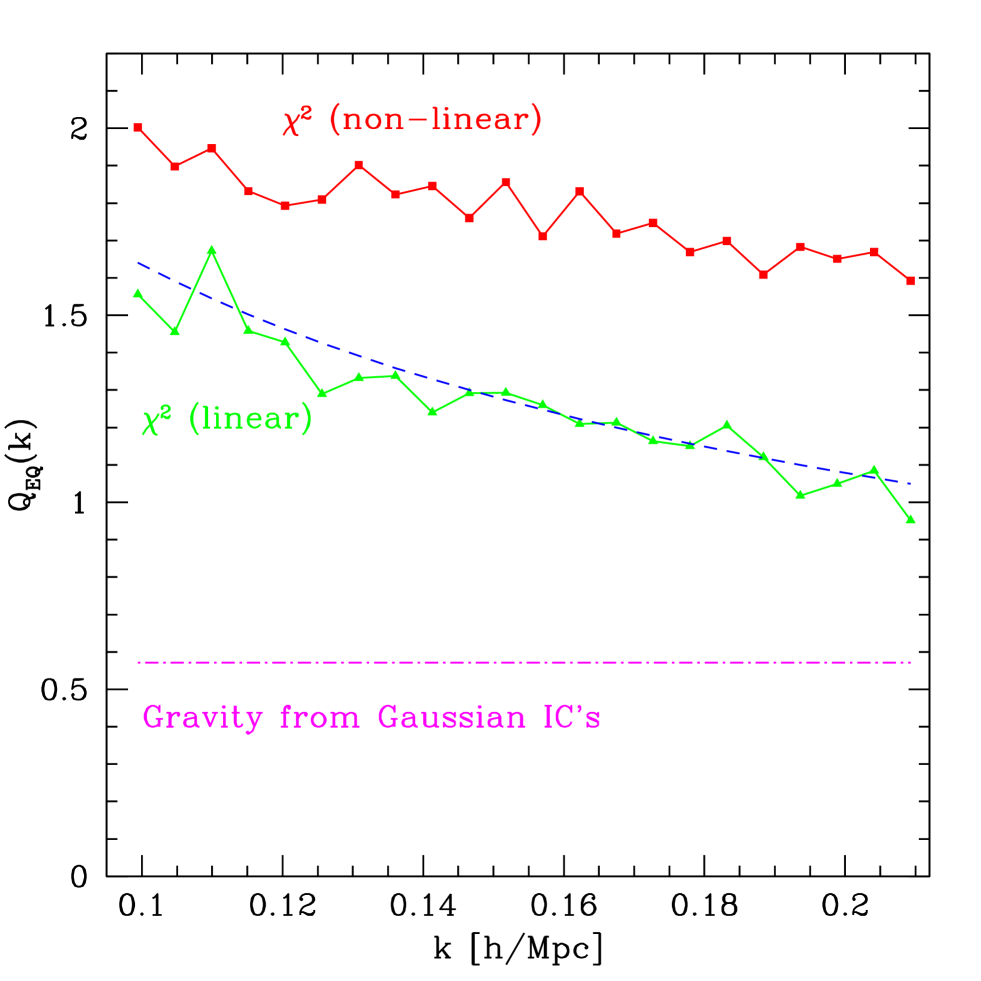
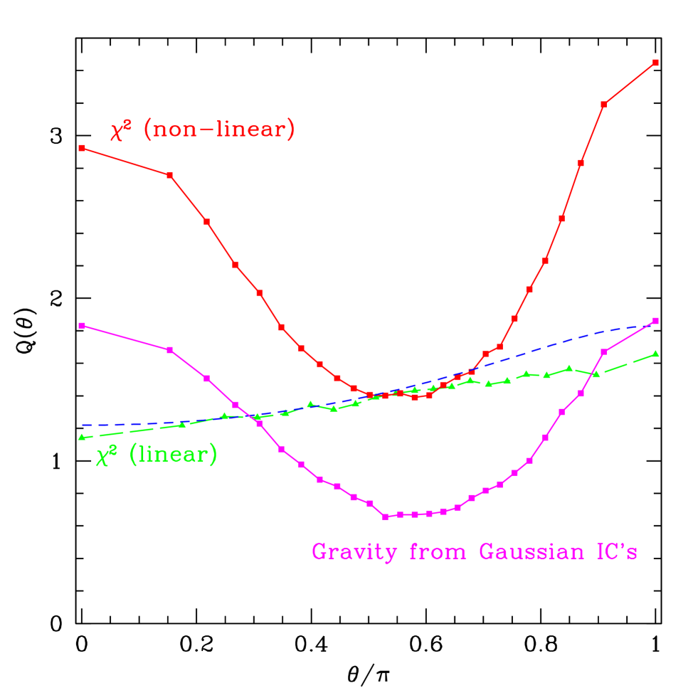
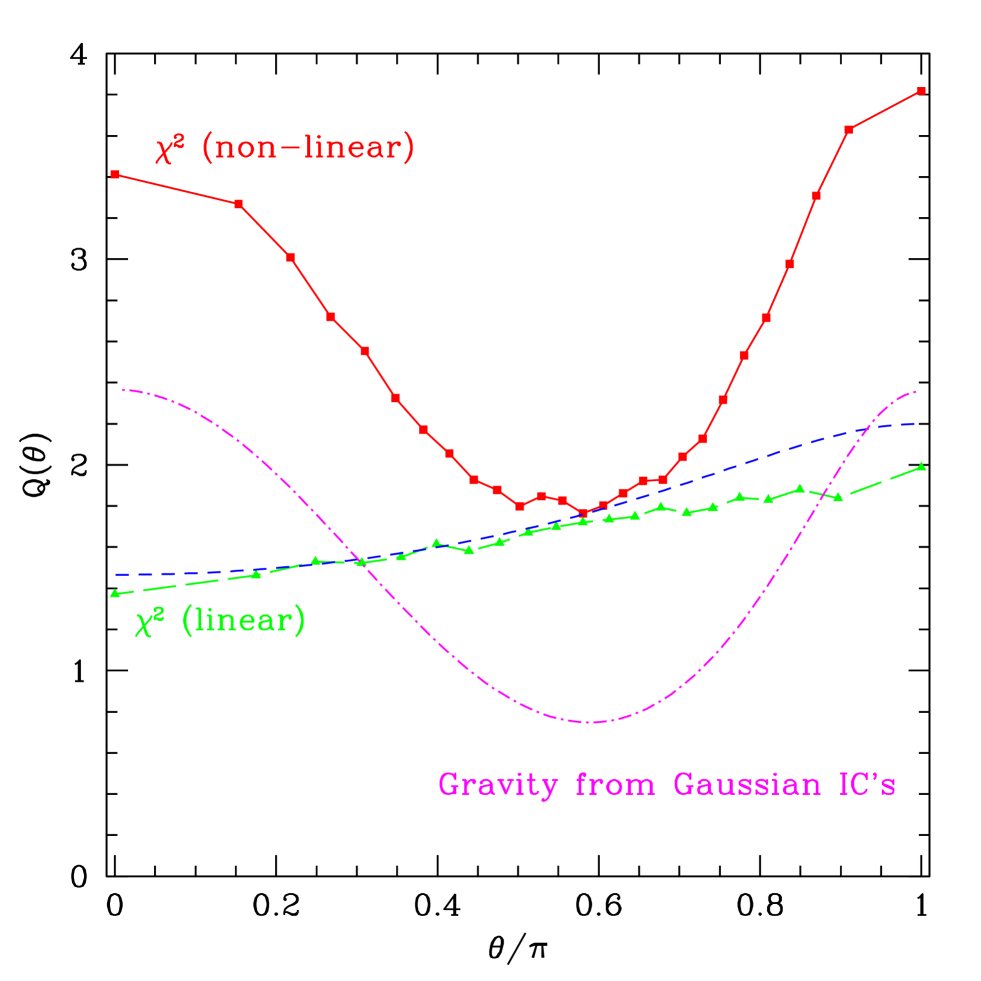
Figures 1 and 2 show the results of 100 2LPT realizations. We have chosen the auxiliary Gaussian field $\phi$ with a spectral index $n_{\phi}=-2.4$, leading to $n=-1.8$ as proposed in Peebles (1999a). The amplitude of the power spectrum has been chosen to give $k_{nl}\equiv 0.33$ h/Mpc. First, we checked that the initial conditions were generated correctly by comparing the power spectrum and the bispectrum with theoretical expectations. The dashed lines in Fig. 1 show the predictions of the first term in Eq. (20) for the reduced bispectrum at $k_{1}=0.068$ h/Mpc, $k_{2}=2k_{1}$, as a function of angle $\theta$ between ${\mathchoice{{\hbox{\BFd k}}}{{\hbox{\BFt k}}}{{\hbox{\BFs k}}}{{\hbox{\BFss k}}}}_{1}$ and ${\mathchoice{{\hbox{\BFd k}}}{{\hbox{\BFt k}}}{{\hbox{\BFs k}}}{{\hbox{\BFss k}}}}_{2}$. This corresponds to $n=-1$, however, it approximately matches the numerical results (triangles, $n=-1.8$). The latter show less dependence on angle, as expected because the scale dependence in the $n=-1.8$ case ($Q^{I}\propto k^{-0.6}$) is weaker than for $n=-1$ ($Q^{I}\propto k^{-1}$). In Fig. 2 we show equilateral configurations as a function of scale for $\chi^{2}$ initial conditions (triangles) and $Q^{I}_{eq}(k)=0.8(k/k_{nl})^{-0.6}$ (dashed lines), where the proportionality constant was chosen to fit the numerical result, this is slightly larger than the prediction in the first term of Eq. (21) for $n=-1$, and closer to the real-space result $Q_{eq}(r)=0.94(r/r_{nl})^{0.6}$.

The behavior of the $\chi^{2}$ bispectrum is notoriously different from that generated by gravity from Gaussian initial conditions for identical power spectrum (dot-dashed lines in Figs. 1-2) (Frieman & Gaztañaga 1999). The structures generated by squaring a Gaussian field roughly correspond to the underlying Gaussian high-peaks which are mostly spherical, thus the reduced bispectrum is approximately flat. In fact, the increase of $Q^{I}$ as $\theta\rightarrow\pi$ seen in Fig.2 is basically due to the scale dependence of $Q^{I}$, i.e. as $\theta\rightarrow\pi$, the side $k_{3}$ decreases and thus $Q^{I}$ increases.

As shown in Eqs. (20-21), non-linear corrections to the bispectrum are significant at the scales of interest, so linear extrapolation of the initial bispectrum is insufficient to make comparison with current observations. The square symbols in Figs. 1 and 2 show the reduced bispectrum after non-linear corrections are included. As a result, the familiar dependence of $Q_{123}$ on the triangle shape due to the dynamics of large-scale structures is recovered (Fig. 1), and the scale dependence shown by $Q^{I}$ is now reduced (Fig. 21). However, the differences between the Gaussian and $\chi^{2}$ case are very obvious: the $\chi^{2}$ evolved bispectrum has an amplitude about 2-4 times larger than that of an initially Gaussian field with the same power spectrum. Furthermore, the $\chi^{2}$ case shows residual scale dependence that reflects the dimensional scaling of the initial conditions. The analogous results for the skewness were obtained using numerical simulations (White 1999) and non-linear PT in the spherical collapse approximation (Gaztañaga & Fosalba 1998). These signatures can be used to test this model against obervations; however, before we can do so we have to test the robustness of these conclusions against the effects of galaxy biasing and redshift distortions.

4 Galaxy Biasing

We now consider the effects of local biasing when initial conditions are non-Gaussian. If we restrict ourselves to scales larger than those relevant to galaxy formation, the galaxy density field can be thought of as a local transformation of the density field smoothed over large enough scales so that $\delta\ll 1$, and thus expanded as (Fry & Gaztañaga 1993)

$$\delta_{g}=b_{1}\delta+\frac{b_{2}}{2}\delta^{2}+\ldots,$$ (27)

which implies the following mapping for the power spectrum and bispectrum

$$P_{g}(k) = b_{1}^{2}P(k)+b_{1}b_{2}\int d^{3}q\ B^{I}({\mathchoice{{\hbox{\BFd k}}}{{\hbox{\BFt k}}}{{\hbox{\BFs k}}}{{\hbox{\BFss k}}}},{\mathchoice{{\hbox{\BFd q}}}{{\hbox{\BFt q}}}{{\hbox{\BFs q}}}{{\hbox{\BFss q}}}}),$$ (28)

$$B_{g}(k_{1},k_{2},k_{3}) = b_{1}^{3}B_{123}+b_{1}^{2}b_{2}\Sigma_{123}^{I}+\frac{3}{2}b_{1}^{2}b_{2}\int d^{3}q\ T_{123}^{I}({\mathchoice{{\hbox{\BFd q}}}{{\hbox{\BFt q}}}{{\hbox{\BFs q}}}{{\hbox{\BFss q}}}}),$$ (29)

where $T_{123}^{I}({\mathchoice{{\hbox{\BFd q}}}{{\hbox{\BFt q}}}{{\hbox{\BFs q}}}{{\hbox{\BFss q}}}})$ denotes the trispectrum $T^{I}({\mathchoice{{\hbox{\BFd k}}}{{\hbox{\BFt k}}}{{\hbox{\BFs k}}}{{\hbox{\BFss k}}}}_{1},{\mathchoice{{\hbox{\BFd k}}}{{\hbox{\BFt k}}}{{\hbox{\BFs k}}}{{\hbox{\BFss k}}}}_{2},{\mathchoice{{\hbox{\BFd q}}}{{\hbox{\BFt q}}}{{\hbox{\BFs q}}}{{\hbox{\BFss q}}}})$ symmetrized over $\{k_{1},k_{2},k_{3}\}$, and $\Sigma_{123}^{I}$ is defined in Eq. (19). The reduced bispectrum then reads

$$Q_{g}=\frac{1}{b_{1}}Q_{123}+\frac{b_{2}^{\rm eff}}{b_{1}^{2}},$$ (30)

where the effective non-linear bias parameter is given by

$$b_{2}^{\rm eff}=b_{2}\ \left[1+\frac{3}{2\Sigma_{123}^{I}}\int d^{3}q\ T_{123}^{I}({\mathchoice{{\hbox{\BFd q}}}{{\hbox{\BFt q}}}{{\hbox{\BFs q}}}{{\hbox{\BFss q}}}})-\frac{Q_{123}^{I}}{\Sigma_{123}^{I}}\left(P_{1}^{I}\int d^{3}q\ B^{I}({\mathchoice{{\hbox{\BFd k}}}{{\hbox{\BFt k}}}{{\hbox{\BFs k}}}{{\hbox{\BFss k}}}}_{2},{\mathchoice{{\hbox{\BFd q}}}{{\hbox{\BFt q}}}{{\hbox{\BFs q}}}{{\hbox{\BFss q}}}})+{\rm cyc.}\right)\right]$$ (31)

The analogous result to Eq. (30) for the case of the skewness was derived by Fry & Scherrer (1994). So far the derivation does not assume any particular non-Gaussian model. In order to compute the effective non-linear bias parameter, we need to make assumptions about the initial bispectrum and trispectrum. The particular form of the convolution integrals in Eq. (31) require knowledge of the three- and four-point functions where two points coincide. Using Eqs.(11-12) we obtain

$$\int d^{3}q\ B^{I}({\mathchoice{{\hbox{\BFd k}}}{{\hbox{\BFt k}}}{{\hbox{\BFs k}}}{{\hbox{\BFss k}}}}_{1},{\mathchoice{{\hbox{\BFd q}}}{{\hbox{\BFt q}}}{{\hbox{\BFs q}}}{{\hbox{\BFss q}}}})=2^{3/2}\sqrt{\xi^{I}(0)}\ P^{I}(k_{1}),$$ (32)

$$\int d^{3}q\ T_{123}^{I}({\mathchoice{{\hbox{\BFd q}}}{{\hbox{\BFt q}}}{{\hbox{\BFs q}}}{{\hbox{\BFss q}}}})=2^{3/2}\sqrt{\xi^{I}(0)}\ B_{123}^{I}+\frac{4}{3}\Sigma_{123}^{I},$$ (33)

so that

$$b_{2}^{\rm eff}=b_{2}\ \left[3-\sqrt{2\xi^{I}(0)}\ Q_{123}^{I}\right]$$ (34)

In this expression, the meaning of $\xi^{I}(0)$ is the following. As we said above, the local bias model in Eq. (27) holds for smoothed fields, so $\xi^{I}(0)$ is the rms density fluctuation at the smoothing scale. The smoothing filter is the Fourier transform, so in this case we should replace $\xi^{I}(0)\approx\Delta^{I}(k)$ for the average scale $k\approx(k_{1}+k_{2}+k_{3})/3$ under consideration. Using Eq. (18) and Eq. (20) we find

$$b_{2}^{\rm eff}\approx(3-\frac{8}{\sqrt{3}\pi})\ b_{2}\approx 1.53\ b_{2}$$ (35)

Thus, for $\chi^{2}$ initial conditions, the usual Gaussian initial conditions biasing formula is recovered (with no additional scale or configuration dependence) provided a proper redefinition of the non-linear bias parameter is made. Note that for other spectral indices than $n=-1$, the resulting $b_{2}^{\rm eff}$ remains independent of scale. In principle, there could be some residual dependence on triangle configuration; however, for $n=-1.8$ the 2LPT results described above give negligible residual configuration dependence as well.

5 Redshift Distortions

In redshift space, the radial coordinate s of a galaxy is given by its observed radial velocity, a combination of its Hubble flow plus “distortions” due to peculiar velocities. The mapping from real-space position x to redshift space is given by:

$${\mathchoice{{\hbox{\BFd s}}}{{\hbox{\BFt s}}}{{\hbox{\BFs s}}}{{\hbox{\BFss s}}}}={\mathchoice{{\hbox{\BFd x}}}{{\hbox{\BFt x}}}{{\hbox{\BFs x}}}{{\hbox{\BFss x}}}}-f\ {\hbox{$u_{z}$}}({\mathchoice{{\hbox{\BFd x}}}{{\hbox{\BFt x}}}{{\hbox{\BFs x}}}{{\hbox{\BFss x}}}}){\hat{z}},$$ (36)

where $f=d\ln D_{1}/d\ln a\approx\Omega^{0.6}$, and ${\mathchoice{{\hbox{\BFd u}}}{{\hbox{\BFt u}}}{{\hbox{\BFs u}}}{{\hbox{\BFss u}}}}({\mathchoice{{\hbox{\BFd x}}}{{\hbox{\BFt x}}}{{\hbox{\BFs x}}}{{\hbox{\BFss x}}}})\equiv-{\mathchoice{{\hbox{\BFd v}}}{{\hbox{\BFt v}}}{{\hbox{\BFs v}}}{{\hbox{\BFss v}}}}({\mathchoice{{\hbox{\BFd x}}}{{\hbox{\BFt x}}}{{\hbox{\BFs x}}}{{\hbox{\BFss x}}}})/({\cal H}f)$, where ${\mathchoice{{\hbox{\BFd v}}}{{\hbox{\BFt v}}}{{\hbox{\BFs v}}}{{\hbox{\BFss v}}}}({\mathchoice{{\hbox{\BFd x}}}{{\hbox{\BFt x}}}{{\hbox{\BFs x}}}{{\hbox{\BFss x}}}})$ is the peculiar velocity field, and ${\cal H}(\tau)\equiv(1/a)(da/d\tau)=Ha$ is the conformal Hubble parameter (with FRW scale factor $a(\tau)$ and conformal time $\tau$). In Eq. (36), we have assumed the “plane-parallel” approximation, so that the line-of-sight is taken as a fixed direction, denoted by ${\hat{z}}$. Using this mapping, the Fourier transform of the density field contrast in redshift space reads (Scoccimarro et al. 1999)

$$\delta_{s}({\mathchoice{{\hbox{\BFd k}}}{{\hbox{\BFt k}}}{{\hbox{\BFs k}}}{{\hbox{\BFss k}}}})=\int\frac{d^{3}x}{(2\pi)^{3}}{\rm e}^{-i{\mathchoice{{\hbox{\BFd k}}}{{\hbox{\BFt k}}}{{\hbox{\BFs k}}}{{\hbox{\BFss k}}}}\cdot{\mathchoice{{\hbox{\BFd x}}}{{\hbox{\BFt x}}}{{\hbox{\BFs x}}}{{\hbox{\BFss x}}}}}{\rm e}^{ifk_{z}{\hbox{$u_{z}$}}({\mathchoice{{\hbox{\BFd x}}}{{\hbox{\BFt x}}}{{\hbox{\BFs x}}}{{\hbox{\BFss x}}}})}\Big{[}\delta({\mathchoice{{\hbox{\BFd x}}}{{\hbox{\BFt x}}}{{\hbox{\BFs x}}}{{\hbox{\BFss x}}}})+f\nabla_{z}{\hbox{$u_{z}$}}({\mathchoice{{\hbox{\BFd x}}}{{\hbox{\BFt x}}}{{\hbox{\BFs x}}}{{\hbox{\BFss x}}}})\Big{]}.$$ (37)

This equation describes the fully non-linear density field in redshift space in the plane-parallel approximation. In linear perturbation theory, the exponential factor becomes unity, and we recover the well known formula (Kaiser 1987)

$$\delta_{s}({\mathchoice{{\hbox{\BFd k}}}{{\hbox{\BFt k}}}{{\hbox{\BFs k}}}{{\hbox{\BFss k}}}})=\delta({\mathchoice{{\hbox{\BFd k}}}{{\hbox{\BFt k}}}{{\hbox{\BFs k}}}{{\hbox{\BFss k}}}})\ (1+f\mu^{2}),$$ (38)

where $\mu\equiv k_{z}/k$. Redshift distortions are trivial to include for $Q^{I}_{123}$, since only linear PT is involved. Assuming linear biasing, Eq. (38) gives the monopole of the reduced bispectrum

$$Q^{I}_{s\ 123}=\frac{\overline{(1+\beta\mu_{1}^{2})(1+\beta\mu_{2}^{2})(1+\beta\mu_{3}^{2})}}{(1+2\beta/3+\beta^{2}/5)^{2}}\times\frac{Q^{I}_{123}}{b_{1}}\equiv A_{s}\frac{Q^{I}_{123}}{b_{1}},$$ (39)

where $\beta\equiv f/b_{1}$, $\mu_{i}k_{i}\equiv{\mathchoice{{\hbox{\BFd k}}}{{\hbox{\BFt k}}}{{\hbox{\BFs k}}}{{\hbox{\BFss k}}}}_{i}\cdot\hat{z}$ and the bar denotes angular average over triangle orientations. Note that this results holds irrespective of the type of non-Gaussian initial conditions. After some algebra, we obtain $A_{s}=C_{s}/(1+2\beta/3+\beta^{2}/5)^{2}$ with

$$C_{s}=1+\beta+\frac{2}{5}\beta^{2}+\frac{2}{35}\beta^{3}+\frac{\beta^{2}(7+3\beta)}{210}\left[\frac{k_{1}^{6}+k_{2}^{6}+k_{3}^{6}-k_{1}^{4}k_{2}^{2}-k_{1}^{2}k_{2}^{4}-k_{1}^{4}k_{3}^{2}-k_{2}^{4}k_{3}^{2}-k_{1}^{2}k_{3}^{4}-k_{2}^{2}k_{3}^{4}}{k_{1}^{2}k_{2}^{2}k_{3}^{2}}\right]$$ (40)

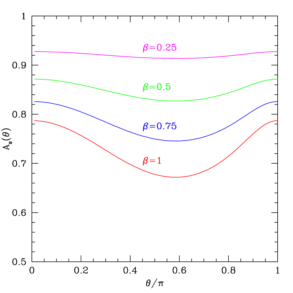
In Fig. 3 we show the correction factor for redshift distortions $A_{s}$. Unlike the Gaussian initial conditions case, where the redshift-space correction is only about $10\%$ (Hivon et al. 1995), for non-Gaussian models it can be significantly more, depending on the value of $\beta$. The reason is simply due to the scaling of the primordial bispectrum being dimensional rather than hierarchical (as that generated by gravity from Gaussian initial conditions). That is, from Eq. (39) one expects that approximately $A_{s}\approx 1/\sqrt{1+2/3\beta+\beta^{2}/5}$, which describes very well the mean value of $A_{s}$ shown in Fig. 3.

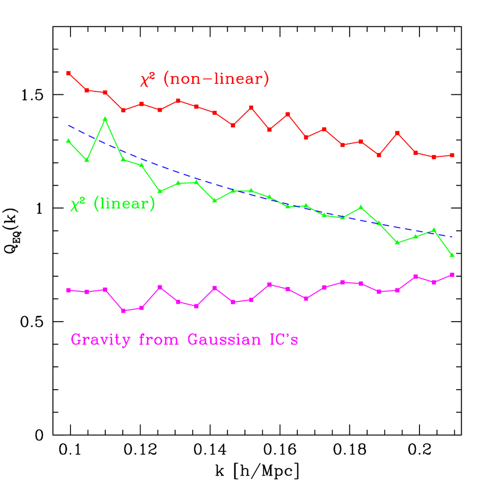
As seen from Eq. (37), the density field in redshift-space is exponentially sensitive to the velocity field. Thus, expanding this effect by linear PT is only valid at very large scales. In order to incorporate the non-linear effects of the redshift-space mapping, we ran 2LPT realizations in redshift space, which take into account this mapping exactly. We assume a cosmological model with $\Omega=0.3$ and $\Omega_{\Lambda}=0.7$, for which $\beta\approx 0.51$. Figures 4 and 5 show the results corresponding to the same triangles as in Figs. 1 and 2, respectively. The amplitudes in redshift space are changed, but the overall behavior is the same: the $\chi^{2}$ model shows larger bispectrum amplitude and scale dependence than the Gaussian initial conditions case. Note that 2LPT calculations in the latter case also automatically include non-linear effects besides those due to redshift-space distortions (“loop corrections”), which were not present in the predictions shown as dot-dashed lines in Figs. 1 and 2; this explains the mild scale dependence of the equilateral bispectrum in Fig. 5 opossite to that of the $\chi^{2}$ model. In summary, we conclude that the results of Section 3 are robust against the effects of redshift distortions.

Another signature of primordial non-Gaussianity is provided by the redshift-space power spectrum. As we discussed above, when initial conditions are non-Gaussian, new couplings become available and non-linear corrections become important at larger scales than in the Gaussian initial conditions case. In redshift-space, this manifests itself in a particular way, as we now discuss. Consider the redshift-space power spectrum, from Eq. (37) we can write a simple expression for the power spectrum in redshift space (Scoccimarro et al. 1999)

$$P_{s}(k,\mu)=\int\frac{d^{3}r}{(2\pi)^{3}}{\rm e}^{-i{\mathchoice{{\hbox{\BFd k}}}{{\hbox{\BFt k}}}{{\hbox{\BFs k}}}{{\hbox{\BFss k}}}}\cdot{\mathchoice{{\hbox{\BFd r}}}{{\hbox{\BFt r}}}{{\hbox{\BFs r}}}{{\hbox{\BFss r}}}}}\Big{\langle}{\rm e}^{ifk\mu[{\hbox{$u_{z}$}}({\mathchoice{{\hbox{\BFd x}}}{{\hbox{\BFt x}}}{{\hbox{\BFs x}}}{{\hbox{\BFss x}}}})-{\hbox{$u_{z}$}}({\mathchoice{{\hbox{\BFd x}}}{{\hbox{\BFt x}}}{{\hbox{\BFs x}}}{{\hbox{\BFss x}}}}^{\prime})]}\Big{[}\delta({\mathchoice{{\hbox{\BFd x}}}{{\hbox{\BFt x}}}{{\hbox{\BFs x}}}{{\hbox{\BFss x}}}})+f\nabla_{z}{\hbox{$u_{z}$}}({\mathchoice{{\hbox{\BFd x}}}{{\hbox{\BFt x}}}{{\hbox{\BFs x}}}{{\hbox{\BFss x}}}})\Big{]}\Big{[}\delta({\mathchoice{{\hbox{\BFd x}}}{{\hbox{\BFt x}}}{{\hbox{\BFs x}}}{{\hbox{\BFss x}}}}^{\prime})+f\nabla_{z}^{\prime}{\hbox{$u_{z}$}}({\mathchoice{{\hbox{\BFd x}}}{{\hbox{\BFt x}}}{{\hbox{\BFs x}}}{{\hbox{\BFss x}}}}^{\prime})\Big{]}\Big{\rangle},$$ (41)

where ${\mathchoice{{\hbox{\BFd r}}}{{\hbox{\BFt r}}}{{\hbox{\BFs r}}}{{\hbox{\BFss r}}}}\equiv{\mathchoice{{\hbox{\BFd x}}}{{\hbox{\BFt x}}}{{\hbox{\BFs x}}}{{\hbox{\BFss x}}}}-{\mathchoice{{\hbox{\BFd x}}}{{\hbox{\BFt x}}}{{\hbox{\BFs x}}}{{\hbox{\BFss x}}}}^{\prime}$. This is a fully non-linear expression, no approximation has been made except for the plane-parallel approximation. The factors in square brackets denote the amplification of the power spectrum in redshift space due to infall, and they constitute the only contribution in linear PT, giving Kaiser’s (1987) result

$$P_{s}(k,\mu)=(1+f\mu^{2})^{2}P(k).$$ (42)

The anisotropy of the power spectrum in redshift space can be characterized by expanding it in multipole moments with respect to $\mu$, the cosine of the angle between a given wave vector k and the line of sight $\hat{z}$. This gives a monopole $P_{0}(k)=(1+2/3f+f^{2}/5)P(k)$, and quadrupole $P_{2}(k)=(4/3f+4/7f^{2})P(k)$. The quadrupole to monopole ratio $P_{2}/P_{0}$ is thus sensitive to the matter density parameter $\Omega$, in fact, assuming linear bias $P_{2}/P_{0}$ is just a function of $\beta=f/b_{1}$ (Kaiser 1987; Hamilton 1992).

On the other hand, at smaller scales the pairwise velocity along the line of sight in the exponential factor in Eq. (41) starts to play a role. This eventually leads to a decrease in monopole and quadrupole power with respect to the linear contribution; in particular, the quadrupole changes sign and becomes negative. Note that this effect is distinct from that of velocity dispersion associated with clusters which takes place at smaller scales than considered here, and leads to a strong negative quadrupole. In fact, at the scales we work the decrease in the quadrupole to monopole ratio can be understood from perturbative dynamics, as has been noted before (Taylor & Hamilton 1996; Fisher & Nusser 1996; Hui, Kofman & Shandarin 1999; Scoccimarro et al. 1999).

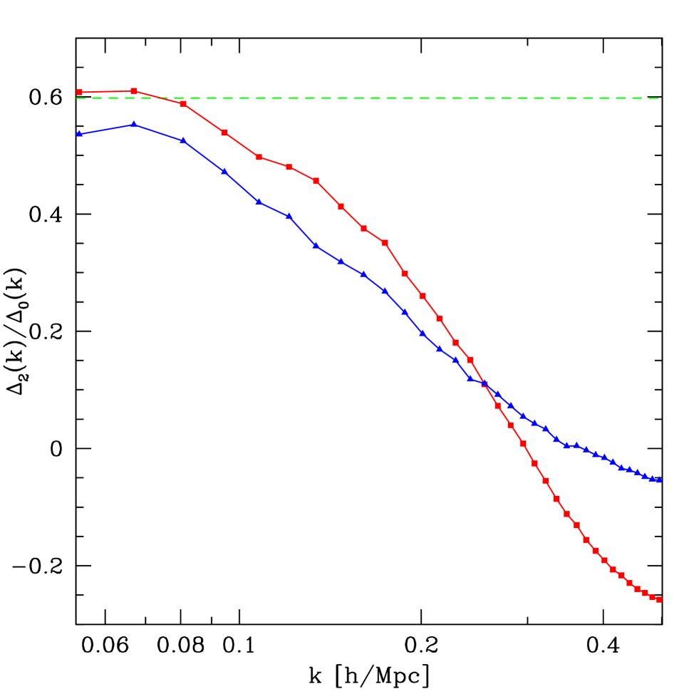
From Eq. (41), one expects that the scale of quadrupole zero crossing is very sensitive to the magnitude of infall velocities. In redshift-space, infall into large-scale structures can become large enough that “near” and “far” sides of large-scale structures in real space reverse sides in redshift-space (Hui et al. 1999). At this point statistical isotropy is recovered and thus the quadrupole vanishes. The magnitude of infall at a given scale $k$ is essentially given by the power spectrum $P_{\theta}(k)$ of the velocity divergence, ($\theta({\mathchoice{{\hbox{\BFd x}}}{{\hbox{\BFt x}}}{{\hbox{\BFs x}}}{{\hbox{\BFss x}}}})\equiv\nabla\cdot{\mathchoice{{\hbox{\BFd u}}}{{\hbox{\BFt u}}}{{\hbox{\BFs u}}}{{\hbox{\BFss u}}}}$), which evolves according to (compare with Eq.6)

$$P_{\theta}(k)=P^{I}(k)+2\int d^{3}q\ G_{2}({\mathchoice{{\hbox{\BFd k}}}{{\hbox{\BFt k}}}{{\hbox{\BFs k}}}{{\hbox{\BFss k}}}}+{\mathchoice{{\hbox{\BFd q}}}{{\hbox{\BFt q}}}{{\hbox{\BFs q}}}{{\hbox{\BFss q}}}},-{\mathchoice{{\hbox{\BFd q}}}{{\hbox{\BFt q}}}{{\hbox{\BFs q}}}{{\hbox{\BFss q}}}})\ B^{I}({\mathchoice{{\hbox{\BFd k}}}{{\hbox{\BFt k}}}{{\hbox{\BFs k}}}{{\hbox{\BFss k}}}},{\mathchoice{{\hbox{\BFd q}}}{{\hbox{\BFt q}}}{{\hbox{\BFs q}}}{{\hbox{\BFss q}}}}),$$ (43)

where the kernel $G_{2}({\mathchoice{{\hbox{\BFd k}}}{{\hbox{\BFt k}}}{{\hbox{\BFs k}}}{{\hbox{\BFss k}}}}_{1},{\mathchoice{{\hbox{\BFd k}}}{{\hbox{\BFt k}}}{{\hbox{\BFs k}}}{{\hbox{\BFss k}}}}_{2})\equiv 3/7+1/2\cos\theta(k_{1}/k_{2}+k_{2}/k_{1})+4/7\cos^{2}\theta$ describes the second-order evolution of the velocity field, similar to $F_{2}$ in Eq. (1) for the density field. Thus, the velocity divergence power spectrum is sensitive to the primordial bispectrum. For the $\chi^{2}$ model with $n=-1$ model as in Section 3 gives (compare with Eq.18)

$$\Delta_{\theta}(k)=\left(\frac{k}{k_{nl}}\right)^{2}\ \left(1-\frac{8}{7\sqrt{2}\pi}\frac{k}{k_{nl}}\right)\approx\left(\frac{k}{k_{nl}}\right)^{2}\ \left(1-0.26\frac{k}{k_{nl}}\right).$$ (44)

Thus, for $\chi^{2}$ initial conditions we expect large-scale infall velocities to be smaller than for Gaussian initial conditions. The effect of primordial non-Gaussianity on the pairwise velocity distribution has been explored by Catelan & Scherrer (1995).

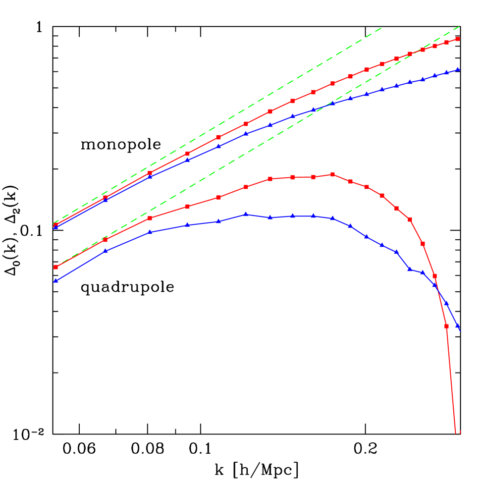
Figures 6 and 7 show results of 100 2LPT realizations of Gaussian and $\chi^{2}$ initial conditions with spectral index $n=-1.4$, $k_{nl}=0.33$ h/Mpc, $\Omega=0.3$ and $\Omega_{\Lambda}=0.7$. The dashed lines show the predictions of linear PT, Eq. (42). Clearly, non-linear effects are important even at scales as large as $k=0.06$ h/Mpc. Comparing the Gaussian (squares) and the $\chi^{2}$ model (triangles), we see that the $\chi^{2}$ model shows a smaller amplification and the zero crossing of the quadrupole happens at smaller scales, consistent with infall velocities being smaller as described above. In fact, the quadrupole has not yet reached its large-scale limit at $k=0.06$h/Mpc. We have checked that this result is not an artifact by verifying that lowering the power spectrum normalization brings the quadrupole to agreement with linear PT. Therefore, the shape of the quadrupole to monopole ratio is sensitive to primordial non-Gaussianity, in this case becoming flatter than the corresponding Gaussian model with the same power spectrum. At small scales sensitive to virial motions inside clusters, however, we expect a different behavior. Models with primordial positive skewness such as the $\chi^{2}$ model tend to have more prominent “fingers of god” (Weinberg & Cole 1992).

6 Conclusions

We have explored the predictions of $\chi^{2}$ initial conditions for clustering statistics, in particular the power spectrum and bispectrum. We found that extrapolation of the initial conditions using linear perturbation theory is not accurate enough at the scales best probed by current and future galaxy redshift surveys ($k\mathrel{\mathchoice{\lower 3.6pt\vbox{\halign{$\mathsurround=0pt\displaystyle\hfill#\hfil$\cr>\crcr\sim\crcr}}}{\lower 3.6pt\vbox{\halign{$\mathsurround=0pt\textstyle\hfill#\hfil$\cr>\crcr\sim\crcr}}}{\lower 3.6pt\vbox{\halign{$\mathsurround=0pt\scriptstyle\hfill#\hfil$\cr>\crcr\sim\crcr}}}{\lower 3.6pt\vbox{\halign{$\mathsurround=0pt\scriptscriptstyle\hfill#\hfil$\cr>\crcr\sim\crcr}}}}0.05$ h/Mpc). This is not surprising, non-Gaussian initial conditions provide additional non-linear couplings otherwise forbidden by symmetry, thus non-linear gravitational corrections can become important at larger scales than in the Gaussian case.

We showed that when non-linear corrections are included, the bispectrum shows a similar configuration dependence as in the Gaussian case; however its amplitude is much larger than the latter and has a residual scale dependence not present in evolution from Gaussian initial conditions. We included the effects of galaxy biasing and showed that the galaxy bispectrum obeys the same relation to the dark matter bispectrum as in the Gaussian case with a proper redefinition of the non-linear bias parameter. Thus, a large linear bias decreases the dependence of the bispectrum on triangle configuration, and a non-linear bias contributes a constant independent of configuration just as in the Gaussian case. The effects of redshift distortions were shown to change the overall amplitude of Gaussian and non-Gaussian bispectra, but clear difference between them remains. Thus, we conclude that the bispectrum is a very useful statistic to probe the Gaussianity of initial conditions, at least for models where the scaling is dimensional as in the $\chi^{2}$ case. Application of these results to current galaxy surveys will be reported elsewhere (Scoccimarro et al. 2000).

We also discussed the effects of non-Gaussianity on the power spectrum in redshift space. The shape of the quadrupole to monopole ratio is very sensitive to the large-scale pairwise velocity which depends on the primordial bispectrum through non-linear corrections. For the $\chi^{2}$ model, this leads to a smaller infall velocity and thus a supression of overall power and smaller quadrupole zero crossing scale compared to the case of Gaussian initial conditions. This provides an additional signature of primordial non-Gaussianity that can be explored with the future generation of galaxy redshift surveys.

Figure 1: The reduced bispectrum $Q$ for triangles with sides $k_{1}=0.068$ h/Mpc and $k_{2}=2k_{1}$ as a function of the angle $\theta$ between ${\mathchoice{{\hbox{\BFd k}}}{{\hbox{\BFt k}}}{{\hbox{\BFs k}}}{{\hbox{\BFss k}}}}_{1}$ and ${\mathchoice{{\hbox{\BFd k}}}{{\hbox{\BFt k}}}{{\hbox{\BFs k}}}{{\hbox{\BFss k}}}}_{2}$. Triangles denote linear extrapolation from $\chi^{2}$ initial conditions, whereas square symbols show the result of non-linear evolution. Dot-dashed lines show the predictions of non-linear PT from Gaussian initial conditions with the same initial power spectrum as the $\chi^{2}$ model.

Figure 2: The reduced bispectrum for equilateral triangles as a function of scale $k$. Line styles as in Fig. 1.

Figure 3: The correction factor for redshift distortions to the primordial bispectrum, $A_{s}$, as a function of angle $\theta$ between ${\mathchoice{{\hbox{\BFd k}}}{{\hbox{\BFt k}}}{{\hbox{\BFs k}}}{{\hbox{\BFss k}}}}_{1}$ and ${\mathchoice{{\hbox{\BFd k}}}{{\hbox{\BFt k}}}{{\hbox{\BFs k}}}{{\hbox{\BFss k}}}}_{2}$ for triangles with sides $k_{1}/k_{2}=2$, for different values of $\beta\approx\Omega^{0.6}/b_{1}$.

Figure 4: Same as Fig. 1 but in redshift space.

Figure 5: Same as Fig. 2 but in redshift space.

Figure 6: The power spectrum monopole (top set of curves) and quadrupole (bottom) as a function of scale for scale-free initial spectra $n=-1.4$ for Gaussian (squares) and $\chi^{2}$ initial conditions (triangles). The dashed lines show the predictions of linear PT.

Figure 7: The power spectrum quadrupole to monopole ratio $\Delta_{2}/\Delta_{0}$ as a function of scale for scale-free initial spectra $n=-1.4$ for Gaussian (squares) and $\chi^{2}$ initial conditions (triangles). The horizonal line denotes the large-scale limit expected in linear perturbation theory.

References

• (1) Antoniadis I., Mazur P. O., Mottola E. 1997, Phys. Rev. Lett., 79, 14
• (2) Bouchet F.R., Colombi S., Hivon E., Juszkiewicz R. 1995, A&A, 296, 575
• (3) Buchert T., Melott A. L., Weiβ𝛽\beta A. G. 1994, A&A, 288, 349
• (4) Catelan, P., & Scherrer, R. J. 1995, ApJ, 445, 1
• (5) Chodorowski, M.J., & Bouchet, F.R. 1996, MNRAS, 279, 557
• (6) Coles, P., Moscardini, L., Lucchin, F., Matarrese, S., & Messina, A. 1993, MNRAS, 264, 749
• (7) Feldman H.A., Kaiser N., Peacock J. 1994, ApJ, 426, 23
• (8) Fisher, K., & Nusser, A., 1996, MNRAS, 279, L1
• (9) Frieman, J.A., & Gaztañaga, E. 1999, ApJ, 521, L83
• (10) Fry, J.N. 1984, ApJ, 279, 499
• (11) Fry, J. N., & Gaztañaga, E. 1993, ApJ, 413, 447
• (12) Fry, J.N., & Scherrer, R.J. 1994, ApJ, 429, 36
• (13) Gaztañaga, E., & Mähönen, P. 1996, ApJ, 462, L1
• (14) Gaztañaga, E., & Fosalba, P. 1998, MNRAS, 301, 524
• (15) Hamilton, A. J. S. 1992, ApJ, 385, L5
• (16) Hivon, E., Bouchet, F. R., Colombi, S., & Juszkiewicz, R. 1995, A&A, 298, 643
• (17) Hui, L., Kofman, L., & Shandarin, S. F. 1999, astro-ph/9901104
• (18) Jaffe, A. 1994, Phys. Rev. D, 49, 3893
• (19) Kaiser, N. 1987, MNRAS, 277, 1
• (20) Kofman, L., Blumenthal, G. R., Hodges, H., & Primack, J. R. 1989, in “Large-Scale Structures and Peculiar Motions in the Universe”, eds. Latham, D. W., & da Costa, L. A. N., 339
• (21) Koyama, K., Soda, J., & Taruya, A. 1999, astro-ph/9903027
• (22) Linde, A.D., & Muhanov, V. 1997, Phys. Rev. D, 56, 535
• (23) Moscardini, L., Matarrese, S., Lucchin, F., & Messina, A. 1991, MNRAS, 248, 424
• (24) Peebles, P.J.E., 1997, ApJ, 483, L1
• (25) Peebles, P.J.E., 1999a, ApJ, 510, 523
• (26) Peebles, P.J.E., 1999b, ApJ, 510, 531
• (27) Pierpaoli, E., García-Bellido, J., & Borgani, S. 1999, hep-ph/9909420
• (28) Robinson, J., Gawiser, E., & Silk, J. 1999, astro-ph/9906156
• (29) Scoccimarro, R. 1997, ApJ, 487, 1
• (30) Scoccimarro, R. 1998, MNRAS, 299, 1097
• (31) Scoccimarro, R., Couchman H. M. P., & Frieman J. A. 1999, ApJ, 517, 531
• (32) Scoccimarro, R. 2000, in preparation
• (33) Scoccimarro, R., Feldman, H., Fry, J. N., Frieman, J. A. 2000, in preparation
• (34) Stirling, A. J., Peacock, J. A. 1996, MNRAS, 283, L99
• (35) Sutherland, W., Tadros, H., Efstathiou, G., Frenk, C. S., Keeble, O., Maddox, S., McMahon, R. G., Oliver, S., Rowan-Robinson, M., Saunders, W. & White, S. D. M. 1999, MNRAS, 308, 289
• (36) Taylor, A. N., & Hamilton, A. J. S., 1996, MNRAS, 282, 767
• (37) Turok, N., & Spergel, D. N. 1991, Phys. Rev. Lett., 66, 3093
• (38) Verde, L., Wang, L., Heavens, A.F., & Kamionkowski, M. 1999, astro-ph/9906301
• (39) Weinberg, D., Cole, S. 1992, MNRAS, 259, 652
• (40) White, M. 1999, MNRAS, 310, 511
• (41) Willick, J. A. 1999, astro-ph/9904367
Refer to caption
Figure 1: The reduced bispectrum Q𝑄Q for triangles with sides k1=0.068subscript𝑘10.068k_{1}=0.068 h/Mpc and k2=2k1subscript𝑘22subscript𝑘1k_{2}=2k_{1} as a function of the angle θ𝜃\theta between k1subscriptk1{\mathchoice{{\hbox{\BFd k}}}{{\hbox{\BFt k}}}{{\hbox{\BFs k}}}{{\hbox{\BFss k}}}}_{1} and k2subscriptk2{\mathchoice{{\hbox{\BFd k}}}{{\hbox{\BFt k}}}{{\hbox{\BFs k}}}{{\hbox{\BFss k}}}}_{2}. Triangles denote linear extrapolation from χ2superscript𝜒2\chi^{2} initial conditions, whereas square symbols show the result of non-linear evolution. Dot-dashed lines show the predictions of non-linear PT from Gaussian initial conditions with the same initial power spectrum as the χ2superscript𝜒2\chi^{2} model.