Point source models for the gravitational lens B1608+656: Indeterminacy in the prediction of the Hubble constant

Abstract

We apply elliptical isothermal mass models to reproduce the point source properties, i.e. image positions, flux density ratios and time delay ratios, of the quadruple lens B1608+656. A wide set of suitable solutions is found, showing that models that only fit the properties of point sources are under-constrained and can lead to a large uncertainty in the prediction of H_∘. We present two examples of models predicting H${}_{\circ}\!=\!100{\rm km\,s^{\!-\!1}Mpc^{\!-\!1}}$ ($\chi^{2}\!=\!4$) and H${}_{\circ}\!=\!69{\rm km\,s^{\!-\!1}Mpc^{\!-\!1}}$ ($\chi^{2}\!=\!24$).

1 Introduction

Relative positions, flux ratios and time delays of the 4 images in B1608+656 have been presented here by Fassnacht (1999) and references therein (cf Table 2). Koopmans & Fassnacht (1999) have concluded H${}_{\circ}\!=\!59^{+7}_{-6}{\rm km\,s^{\!-\!1}Mpc^{\!-\!1}}$ within the context of a family of parametrized, isothermal models. Here, we investigate whether a larger set of models allows a wider range of Hubble constants.

2 Elliptical isothermal models

Following Blandford & Kundić (1997), we adopt a scaled lensing potential $\psi$ composed of two elliptical contributions to describe the lensing galaxies G1 and G2 plus external shear $\gamma$:

$$\psi_{=}\sum_{i=1}^{2}\,\,b_{i}\,\{s_{i}^{2}+r_{i}^{2}\,[1-e_{i}\,\cos(2(\varphi_{i}-\phi_{i}))]\}^{1\over 2}+r_{1}^{2}\,\gamma\,\cos(2(\varphi_{1}-\varphi_{\gamma}))$$ (1)

Here $(r_{i},\varphi_{i})$ are polar coordinates with origin at the center of each galaxy. $s$ measures the core radius, $e$ and $\phi$ the ellipticity and position angle of the major axis. At large radius the mass distribution is isothermal, going as $\Sigma\propto r^{-1}$. The lenses will be fixed at $\vec{x}_{G1}\!=\!(0.446,-1.063)^{\prime\prime}$ and $\vec{x}_{G2}\!=\!(-0.276,-0.937)^{\prime\prime}$, the centroids in H band, which are less affected by reddening (Blandford, Surpi & Kundić 1999).

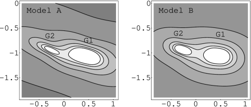
We minimize a $\chi^{2}$ function. The best fit achieved, hereafter Model A, has $\chi^{2}\!=\!4.0$ and yields $H_{\circ}\!=\!100{\rm km\,s^{\!-\!1}Mpc^{\!-\!1}}$. Models with lower values of $H_{\circ}$ can also be built fixing $H_{\circ}$ and fitting the 3 time delays instead of the time delay ratios. As an example we present the results of Model B having $H_{\circ}\!=\!69{\rm km\,s^{\!-\!1}Mpc^{\!-\!1}}$ and $\chi^{2}\!=\!24.7$. The parameters and predictions of Model A and B are displayed in Tables 2 and 2 respectively. They represent reasonable mass distributions given, especially, our ignorance of the dark matter distribution (Figure 1).

3 Discussion

A variety of parametrized models can reproduce the point source properties of B1608+656. This precludes an accurate determination of H_∘. To break the degeneracy, extra constraints, associated with the extended emission of the source, have to be incorporated. It is also helpful to specify the distribution of dark matter on larger scale than the image distribution. A similar conclusion has been drawn by Williams & Saha (1999) using pixellated models.

Figure 1: Surface mass density in Models A and B

Table 1: Model parameters.

	Model A (H${}_{\circ}\!=\!100\scriptstyle\rm km\,s^{\!-\!1}Mpc^{\!-\!1}$)		Model B (H${}_{\circ}\!=\!69\scriptstyle\rm km\,s^{\!-\!1}Mpc^{\!-\!1}$)
Parameters	G1	G2	G1	G2
s(”)	0.10	0.10	0.00	0.05
b	0.9072	0.2453	0.7797	0.3429
e	0.3269	0.6405	0.1570	0.3149
$\phi(^{\circ})$	163.45	154.93	172.62	160.86
$\gamma,\varphi_{\gamma}(^{\circ})$	0.0876	-10.92	0.0473	12.47

Table 2: Comparison between observations and model predictions.

Properties	Observation	Model A	Model B
$\vec{x}_{A}(^{\prime\prime})$	( 0.0000, 0.0000) $\pm$ (0.0023,0.0023)	( 0.0000, 0.0000)	( 0.0000, 0.0000)
$\vec{x}_{B}(^{\prime\prime})$	(-0.7380,-1.9612) $\pm$ (0.0043,0.0046)	(-0.7382,-1.9613)	(-0.7365,-1.9518)
$\vec{x}_{C}(^{\prime\prime})$	(-0.7446,-0.4537) $\pm$ (0.0045,0.0049)	(-0.7443,-0.4544)	(-0.7422,-0.4575)
$\vec{x}_{D}(^{\prime\prime})$	( 1.1284,-1.2565) $\pm$ (0.0107,0.0124)	( 1.1271,-1.2582)	( 1.1269,-1.2207)
$F_{A}/F_{B}$	2.042 $\pm$ 0.124	1.917	1.901
$F_{C}/F_{B}$	1.037 $\pm$ 0.083	1.092	1.131
$F_{D}/F_{B}$	0.350 $\pm$ 0.055	0.428	0.504
$T_{AB}(d)$	26.0 $\pm$ 5.0	28.4	27.6
$T_{CB}(d)$	33.0 $\pm$ 5.0	32.0	31.7
$T_{DB}(d)$	73.0 $\pm$ 5.0	68.4	71.3
$\chi^{2}$	0.0	4.0	24.7

References

- [1] landford, R., & Kundic, T. 1996 The Extragalactic Distance Scale, p60
- [2] landford, R., Surpi, G. & Kundić, T. 1999 these proceedings
- [3] assnacht, C. 1999 these proceedings
- [4] oopmans, L.V., & Fassnacht, C.D. 1999 astro-ph/9907258, to appear in ApJ
- [5] illiams, L. L. R. & Saha, P. 1999 these proceedings