Accelerations of Water Masers in NGC4258

Abstract

The water masers in NGC4258 delineate the structure and dynamics of a sub-parsec-diameter accretion disk around a supermassive black hole. VLBA observations provide precise information about the positions in the plane of the sky and the three-dimensional velocity vectors for the maser emission, but the positions along the line of sight must be inferred from models. Previous measurements placed an upper limit on the accelerations of the high-velocity spectral features of 1 km s^-1yr^-1, suggesting that they are located near the midline (the diameter perpendicular to the line of sight), where they would have exactly zero acceleration. From similar measurements, the accelerations of the systemic-velocity spectral features have been estimated to be about 9 km s^-1yr^-1, indicating that they lie toward the front of the disk where the acceleration vector points directly away from the line of sight. We report acceleration measurements for 12 systemic-velocity spectral features and 19 high-velocity spectral features using a total of 25 epochs of observations from Effelsberg (5 epochs), the VLA (15 epochs), and the VLBA (5 epochs) spanning the years 1994 to 1997. The measured accelerations of the systemic-velocity features are between 7.5 and 10.4 km s^-1yr^-1 and there is no evidence for a dip in the spectrum at the systemic velocity. Such a dip has been attributed in the past to an absorbing layer of non-inverted H₂O (Watson & Wallin 1994; Maoz & McKee 1998). The accelerations of the high-velocity features, measured here for the first time, range from $-0.77$ to 0.38 km s^-1yr^-1. From the line-of-sight accelerations and velocities, we infer the positions of these high-velocity masers with a simple edge-on disk model. The resulting positions fall between $-13.6^{\circ}$ and $9.3^{\circ}$ in azimuth (measured from the midline). A model that suggests a spiral shock origin of the masers (Maoz & McKee 1998), in which changes in maser velocity are due to the outward motion of the shock wave, predicts apparent accelerations of $-0.05(\theta_{p}/2.5^{\circ})$ km s^-1yr^-1, where $\theta_{p}$ is the pitch angle of the spiral arms. Our data are not consistent with these predictions. We also discuss the physical properties of the high-velocity masers. Most notably, the strongest high-velocity masers lie near the midline where the velocity gradient is smallest, thereby providing the longest amplification path lengths.

1 Introduction

Water masers were first detected in the galaxy NGC4258 (M106) by Claussen, Heiligman, & Lo (1984) and Henkel et al. (1984). The $6_{16}-5_{23}$ rotational transition of H₂O, at a rest frequency of 22.235080 GHz, produces this emission. Observers found maser sources spanning a velocity range of about $200\ \mathrm{km\ s^{-1}}$, approximately centered on the systemic velocity of the galaxy, which Cecil, Wilson, & Tully (1992) measured to be $472\pm 4\ \mathrm{km\ s^{-1}}$. (This velocity, along with the rest of the velocities below, uses the radio definition of the Doppler shift, $v/c=\Delta\nu/\nu_{\circ}$, in the LSR frame.) These maser lines are referred to as the systemic-velocity spectral features. The peak flux density varies in time but is generally between 2 and 10 Jy, with a typical value of about 4 Jy. Early Very Long Baseline Interferometry (VLBI) observations of these features revealed that the systemic emission is quite compact, on the order of one-hundredth of a parsec (Claussen et al. 1988), but is elongated with a velocity gradient along its major axis (7970 $\pm$ 40 km s^-1pc^-1), most likely indicative of circular motion seen edge-on (Greenhill et al. 1995a). Haschick & Baan (1990) were the first to note the velocity drift (acceleration) of one systemic feature. Later studies found the whole of the systemic emission to be increasing in velocity at a rate of about 10 km s^-1yr^-1 (Haschick, Baan, & Peng 1994; Greenhill et al. 1995b; Nakai et al. 1995).

Nakai, Inoue, & Miyoshi (1993) observed NGC4258 with a spectrometer of very broad bandwidth and discovered additional maser emission at velocities offset approximately $\pm 1000\ \mathrm{km\ s^{-1}}$ from the previously known systemic emission. These are called the high-velocity spectral features. Unlike the systemic features, which appear as a thicket of overlapping lines, the high-velocity features are more sparse, occurring in small, well-separated clusters of a few narrow ($\sim$ 1 km s^-1), overlapping lines. The redshifted high-velocity features have peak flux densities around 1 Jy or less and have velocities of about 1230 to 1460 $\mathrm{km\ s^{-1}}$. In contrast, the blueshifted high-velocity features have peak flux densities of about 0.1 Jy or less, and cover velocities in the range of $-520$ to $-290$ $\mathrm{km\ s^{-1}}$. In response to the observation of the systemic emission position-velocity gradient, the measurement of the systemic emission velocity drift, and the detection of the high-velocity emission, Watson & Wallin (1994) and Greenhill et al. (1995a) proposed that the systemic- and high-velocity features are all part of a rotating disk about 0.2 pc in radius viewed nearly edge-on. The systemic features originate in a small region on the front side of the disk, producing the linear position-velocity gradient as well as the line-of-sight acceleration observed for these features. The high-velocity features were attributed to gas at large impact parameters where the disk’s orbital motion is parallel to the line of sight. The velocity range of the high-velocity spectrum was believed to reflect the broad radial width of the disk, though the high-velocity maser positions were unknown at this time (Greenhill et al. 1995a).

VLBA observations of both the previously studied systemic features and the more recently discovered high-velocity features provide strong confirmation that the masers are embedded in a rotating disk that we view nearly edge-on (Miyoshi et al. 1995). The results are summarized in Figure Accelerations of Water Masers in NGC4258. The observations show that the features are distributed in a linear fashion with small vertical spread, suggestive of a thin disk. However, the disk is slightly warped; the red- and blueshifted high-velocity features do not precisely “line up,” but rather appear to trace out portions of a curve. The rotation curve inferred from the high-velocity features is Keplerian. The masers are located at disk radii between 0.14 pc and 0.28 pc, and the central mass is 3.9 $\times$ $10^{7}$ M_⊙ for a calculated distance of 7.2 Mpc, most likely in the form of a supermassive black hole (Herrnstein et al. 1999; Maoz 1995a, 1998).

The line-of-sight velocity for a maser in Keplerian rotation around a mass $M$ at a disk radius $R$ is given by $v=\left(\frac{GM}{R}\right)^{1/2}\cos\theta+v_{gal}$, where $\theta$ is the azimuthal position measured from the midline (diameter perpendicular to the line of sight), and $v_{gal}$ is the systemic velocity of the galaxy. Because the masers are well fit by a Keplerian rotation curve, the high-velocity masers must all be located close to a single diameter through the disk, i.e., $\cos\theta$ is a constant. The midline (where $\cos\theta=1$) is the most likely candidate for two reasons. First, the line-of-sight velocity gradient (along the line of sight) is zero there, which maximizes the gain path along which maser amplification can occur. Second, the line-of-sight accelerations measured for the high-velocity features are small (as discussed below).

The line-of-sight velocity for a maser in Keplerian rotation at a disk radius $R$ can also be expressed as $v=\left(\frac{GM}{R}\right)^{1/2}\left(\frac{b}{R}\right)+v_{gal}$, where $b$ is the impact parameter in the plane of the sky measured from the center of the disk. Because the systemic-velocity masers exhibit a linear velocity gradient with impact parameter, they must all be located close to a single disk radius; i.e., $R$ is a constant. The systemic-velocity features are probably located in front of the disk’s dynamical center for two reasons. First, the velocities of these features are near the systemic velocity of the galaxy. Second, these features occur spatially midway between the red- and blueshifted high-velocity features. The distinctly non-zero accelerations measured for the systemic-velocity features are consistent with this interpretation.

Motivated by hints of periodicity in the spacings of high-velocity emission in position and velocity (see Figure Accelerations of Water Masers in NGC4258), Maoz (1995b) proposed that spiral structure is present in the disk and that masing occurs at the density maxima located where the spiral arms intersect the midline. Later, Maoz & McKee (1998) expanded upon this idea and suggested that the disk contains spiral shock waves and that masing occurs only in thin post-shock regions seen in locations where the spiral arms are tangent to the line of sight. In this model the high-velocity features decrease in velocity (magnitude) at a predictable rate, as the spiral structure rotates and different portions of the spiral arms become tangent to the line of sight. Consequently, within the model the masers are not distinct physical entities but rather locations in the disk marking the passage of the spiral excitation wave.

Four previous studies of maser feature accelerations have been made. All four studies measured accelerations for the systemic features; two of the studies also examined high-velocity accelerations. Greenhill et al. (1995b) found accelerations for twelve systemic features using a series of spectra taken at the Effelsberg 100 m telescope in 1984–1986. They measured a range of values between 8.1 and 10.9 $\mathrm{km\ s^{-1}yr^{-1}}$, with an average drift of $9.5\pm 1.1\ \mathrm{km\ s^{-1}yr^{-1}}$. Haschick et al. (1994) observed the systemic features with the Haystack 37 m telescope at roughly monthly intervals from 1986 to 1993. They found accelerations for four clusters of masers of between 6.2 and 10.4 $\mathrm{km\ s^{-1}yr^{-1}}$, with an average value of 7.5 $\mathrm{km\ s^{-1}yr^{-1}}$. Nakai et al. (1995) observed the systemic features with the Nobeyama Radio Observatory 45 m telescope approximately every week in 1992. They measured accelerations for thirteen features of between 8.7 and 10.2 $\mathrm{km\ s^{-1}yr^{-1}}$, with an average rate of $9.6\pm 1.0$ $\mathrm{km\ s^{-1}yr^{-1}}$. All three of the above studies determined the accelerations by following local maxima in spectra through a time series and looking for velocity drifts as a linear function of time. In the fourth study, Herrnstein (1997) used spectra from four epochs of VLBA observations, four to nine months apart. These large time gaps precluded following the features “by eye.” Instead, features were tracked by a Bayesian analysis that considered all possible pairings of features among the epochs. The measured accelerations were between 6.8 and 11.6 km s^-1yr^-1, with most values close to 9 km s^-1yr^-1. The small range in measured acceleration supports the idea that the systemic masers originate in a relatively narrow band of radii.

Two of the previous four studies also examined the high-velocity features, but neither detected any statistically significant accelerations. Greenhill et al. (1995b) measured upper limits of 1 km s^-1yr^-1 for 20 redshifted lines and 3 blueshifted lines in a series of spectra taken in 1993. Nakai et al. (1995) also tracked redshifted and blueshifted spectral lines and found upper limits on the acceleration of 0.7 $\mathrm{km\ s^{-1}yr^{-1}}$ and 2.8  $\mathrm{km\ s^{-1}yr^{-1}}$, respectively.

The purpose of our study was to obtain precise emission feature velocities at regular intervals and thereby measure the accelerations of the high-velocity features. These observations are an improvement over past efforts because of the long time baseline (nearly three years) and frequent observations. The data permit us to derive line-of-sight positions of masers in the disk, to test the predictions of the Maoz & McKee model, and to look for correlations between maser positions and physical properties such as linewidth and intensity.

In §2 we describe the observations and limits on systematic measurement errors, and in §3 we present the measured accelerations. In §4 we compare our results to the Maoz & McKee model, derive maser positions within the disk, and discuss possible correlations in maser properties. A summary of our conclusions is contained in §5. In the appendix we present a quantitative analysis of the relative robustness and sensitivity of maser position estimates obtained individually from measurements of acceleration, position, and line-of-sight velocity. A prelimary version of these results was presented by Bragg et al. (1998).

2 Observations and Data Reduction

This study uses observations from three different instruments: the Very Large Array (VLA) and the Very Long Baseline Array (VLBA) of the NRAO, and the Effelsberg 100 m telescope of the Max Planck Institute for Radio Astronomy. We summarize the observations in Table 1 and display a time-series of systemic, redshifted and blueshifted spectra in Figures Accelerations of Water Masers in NGC4258,  Accelerations of Water Masers in NGC4258, and  Accelerations of Water Masers in NGC4258, respectively.

2.1 VLA Observations

We observed NGC4258 with the VLA seventeen times between 1995 January and 1997 February (approximately every one to two months) in order to obtain a series of spectra of the masers without large time gaps. We used two IFs to observe adjacent velocity ranges. The IFs were tuned to fixed sky frequencies and Doppler tracking was implemented in software. The bandwidth of each IF was 3.125 MHz ($\sim$ 42 km s^-1) which was divided into 128 channels of width 24.4 kHz (0.329 km s^-1). The instantaneous bandwidth for the spectrometer configured in this way is about 80 km s^-1, and a series of seven integrations covered the entire region of interest in the spectrum.

We observed the systemic and redshifted features for all epochs, and the blueshifted features in all but the final three. For all epochs except the first, we observed the systemic features over the range $390$ to $600\ \mathrm{km\ s^{-1}}$, the red features over the range $1235$ to $1460\ \mathrm{km\ s^{-1}}$, and the blue features over the ranges $-460$ to $-420\ \mathrm{km\ s^{-1}}$ and $-390$ to $-350\ \mathrm{km\ s^{-1}}$. (For the first epoch, these ranges were all shifted by $20\ \mathrm{km\ s^{-1}}$ towards higher velocities.) For some epochs, we observed additional velocity bands, including $-550$ to $-510\ \mathrm{km\ s^{-1}}$, $-330$ to $-290\ \mathrm{km\ s^{-1}}$, $1475$ to $1515\ \mathrm{km\ s^{-1}}$, and $1560$ to $1635\ \mathrm{km\ s^{-1}}$, but detected no new emission. Typical integration times for each velocity range were 18 minutes, the exception being the blueshifted velocities, for which we used 36-minute integrations. We observed 1146+399 for phase calibration, 3C286 for flux calibration, and 3C273 for bandpass calibration.

We edited and calibrated the data with standard routines in AIPS. The overall amplitude calibration is accurate to 20% and the relative calibration within each epoch is accurate to 15%. For each epoch, we computed spectra from vector averages of data for all baselines. The angular extent of the maser emission is much smaller than the resolution of the VLA in any configuration, so imaging was unnecessary. For the epoch on 1996 June 27, thunderstorms resulted in the loss of all data. For the epochs on 1995 July 29 and 1995 September 9, large atmospheric phase variations led to the loss of high-velocity data; we recovered part of the systemic data from 1995 July by self-calibration of peaks in the maser spectrum.

2.2 VLBA and Effelsberg Data

The VLBA data we include in this study consist of five spectra of the high-velocity masers taken from 1994 April to 1996 September (Herrnstein 1997, A. Trotter 1998, private communication). For these observations the total bandwidth was $\sim$400 km s ^-1, which was divided into 2048 spectral channels each of width 0.211 km s^-1. The velocity coverage of these observations exceeded that of the VLA spectra, so we have used only the portions that overlap the VLA spectra. As for the VLA data, the amplitude calibration is good to within 20% and Doppler tracking was implemented in software after correlation. The VLBA spectra have better signal-to-noise than the VLA observations largely because the integration times were typically much longer (about 12 hours).

The Effelsberg 100-m telescope data consist of five spectra of the redshifted high-velocity features taken between 1995 March and 1995 June. These observations were obtained in total-power mode with a bandwidth of $\sim$333 km s^-1 divided into 1024 spectral channels of width 0.329 km s^-1. The integration times were between 6 and 12 minutes on-source. These observations covered a velocity range from 1180 to 1510 km s^-1 and the amplitude calibration is accurate to within 20%. We corrected the spectra to the radio definition of the Doppler shift. (We note that by default the band-center velocities of Effelsberg spectra assume the optical definition of the Doppler shift.) At the band-center frequency used, the difference between velocities using the two definition is $-6.052$ km s^-1. The Effelsberg spectra have lower signal-to-noise than those from the VLA largely because of the short integration times.

2.3 Feature Fitting

2.3.1 High-Velocity Features

To measure the velocity of the maser medium for each feature, as well as spectral feature amplitudes and linewidths, we fit Gaussian profiles to the spectral data. However, the high-velocity features occur in clusters of a few partially-overlapping lines so fits of multiple components are necessary. We used a nonlinear, multiple-Gaussian-component least-squares fit. To optimize the fitting, we split the redshifted high-velocity spectra from the VLA and VLBA into three segments, each containing between five and twelve features: from 1225 $\mathrm{km\ s^{-1}}$ to 1300 $\mathrm{km\ s^{-1}}$, from 1300  $\mathrm{km\ s^{-1}}$ to 1375 $\mathrm{km\ s^{-1}}$, and from 1375 $\mathrm{km\ s^{-1}}$ to 1460 $\mathrm{km\ s^{-1}}$. We fit each Effelsberg spectum over the entire 300 km s^-1 range at once as each spectrum contains fewer detectable features because of the lower signal to noise ratios.

Each spectrum was fit iteratively. First, we identified and fit the four or five most prominent peaks. Second, we identified additional features in the residuals by convolving the residuals with a five-channel boxcar function and searching for peaks among these smoothed residuals. Third, we refit the spectrum to include any additional features. We repeated this process until both the rms deviation of the residuals was comparable to the noise level in the spectrum, and no additional features could be picked out “by eye” in the smoothed residuals. Occasionally, we split VLA spectra into 20 to 30 km s^-1 velocity segments (instead of 75 km s^-1) when they were especially crowded.

2.3.2 Systemic Features

We have identified ten to fifteen peaks in each systemic-velocity spectrum. Though it is desirable to obtain velocities from formal fitting, the density of features near the systemic velocity is too great to permit a unique decomposition of the spectra into individual masing components. For these features, we followed the method used by Greenhill et al. (1995b): first, we convolved each spectrum with a three-channel boxcar, second, we identified local maxima and minima, and third, we selected maxima that exceed one of their two neighboring minima by more than $13\sigma$. We have chosen a factor of thirteen to preclude the selection of noise spikes as peaks but to still include most of the visually “real” peaks. This method is not sensitive to lower amplitude peaks but seemed to do reasonably well in the dense part of the spectrum. Because the expected accelerations are greater than for the high-velocity portion of the spectrum, high precision measurement of velocity is less critical.

2.4 Velocity Error Budget

Because the accelerations of the high-velocity features are quite small ($<1$ km s^-1yr^-1), it was important that our individual velocity measurements be accurate to a level not normally needed in radio astronomy. We used a standard routine in AIPS to implement Doppler tracking, for which the uncertainty is $\leq$ 0.004 km s^-1 due to the omission of Jupiter’s influence (The routine accounts for the rotation of the earth, motion of the earth about the earth-moon barycenter, revolution of the earth-moon barycenter about the sun,and the motion of the sun with respect to the local standard of rest.) To verify and possibly to further constrain this uncertainty, we compared sample velocity shifts computed in AIPS to those from the CfA Planetary Ephemermis Program (PEP), which is accurate to 1 mm s^-1 (J. Chandler 1998, private communication). We found the two programs to agree to within the quoted uncertainty of the AIPS routine (0.004 km s^-1). Thus we conclude that any long-term accelerations we observe in the maser features above this level must be due to a real physical effect.

3 Results

3.1 Accelerations of the High-Velocity Maser Features

We have measured accelerations for seventeen redshifted high-velocity features and two blueshifted high-velocity features and find them to range between $-0.77$ and 0.38 km s^-1yr^-1 (Figure Accelerations of Water Masers in NGC4258, Table 2). To do this, we plotted centroid velocity as a function of time for all fitted peaks and identified isolated and minimally-blended features that were resolved by the fitting process described above. We identified three biases in this procedure: (1) features with low accelerations are favored in the presence of blends, (2) feature amplitude and linewidth may be correlated in blends (note the feature at 1450 km s^-1 in Figure Accelerations of Water Masers in NGC4258), and (3) features extremely near each other in velocity with time varying fluxes may appear to be a single feature for which a non-physical acceleration could be measured.

We fit a linear function to the time-series of velocities for each tracked feature and estimate accelerations. The $\chi_{\nu}^{2}$ values derived for these fits are not very good, indicating that the assumption of constant acceleration is not entirely correct. In some cases, the spectral features exhibit a clear systematic wander from constant acceleration, i.e. a “wobble.” The feature at 1306 km s^-1, in particular, exhibits a wander that does not appear to be a result of scatter from measurement error. This “wobble” is likely a result of either feature blending (two nearby features being mistaken for a single feature) or real changes in structure of the masing gas cloud that causes an apparent velocity shift. In any event, the wobble factor is introduced as a source of random noise of unknown amplitude that must be combined with the measurement noise to estimate the acceleration. In order to quantify this “wobble” and find the uncertainties in the acceleration values, we have used a maximum likelihood technique similar to that used to fit simple linear functions, but with the inclusion of a “wobble” uncertainty added in quadrature to the uncertainty in the measurement of the velocity for each feature. This model for the motion of the masers primarily changes the weighting of the measured peak velocities; it is similar to rescaling the errors by $\chi_{\nu}^{2}$, but our method better quantifies the observed deviations in sensible units. In cases like that of the feature at 1306 km s^-1, uncertainty in the estimate of acceleration is almost entirely due to the wobble contribution, where for the feature at -440 km s^-1, the uncertainty is largely due to the measurement errors. The likelihood is given by:

$$P=\prod\frac{1}{\left(\sigma_{i}^{2}+\sigma_{w}^{2}\right)^{\frac{1}{2}}}\exp-\frac{\left(v_{i}-\left(a+bx_{i}\right)\right)^{2}}{2\left(\sigma_{i}^{2}+\sigma_{w}^{2}\right)},$$ (1)

where $i$ enumerates the epochs, $v_{i}$ is the feature velocity measured on day $x_{i}$, with error $\sigma_{i}$, $a$ and $b$ are the usual linear fit parameters (intercept and slope), and $\sigma_{w}$ is the so-called “wobble” factor, which is taken to be constant in time, but different for each feature. We obtained the parameter values that result in the maximum likelihood by taking derivatives of $\ln P$ with respect to $a$, $b$, and $\sigma_{w}$, setting them equal to zero, and solving iteratively to find the acceleration ($b$) and “wobble” factor ($\sigma_{w}$) for each feature. Finally, we estimated the uncertainties by executing a linear least-squares fit with $\sigma_{w}$ held fixed. Note that the units of the wobble factors listed in Table 2 are km s^-1. On the simple assumption that the measurements are approximately uniformly distributed over the three years of observations, the contribution of the wobble to the uncertainty in the measured acceleration will be about 0.3 x $\sigma_{w}$ km s^-1$yr^{-1}$. For cases where this term approaches the measurement uncertainty quoted for the acceleration, the uncertainty is due mostly to the wobble contribution. When the term is small, the uncertainty is due predominantly to measurement error.

3.2 Accelerations of the Systemic-Velocity Features

We have measured accelerations for twelve systemic-velocity features, that are between 7.5 and 10.4 km s^-1yr^-1. As in the case of the high-velocity features, we tracked the emission lines by eye in a plot of velocity versus time for local maxima in the spectra. A linear straight-line least-squares fit to the data for each feature yields an acceleration. We assumed an error of 0.3 km s^-1 for each maximum (corresponding to the width of the velocity channels). Table 3 contains the results of these fits and Figure Accelerations of Water Masers in NGC4258 shows the data and the fitted lines. The range of accelerations agrees well with those obtained by past studies. The average value is 9.1$\pm$0.8 km s^-1yr^-1, where 0.8 km s^-1yr^-1 is the rms deviation from the mean.

It has been proposed that there is a persistent gap or dip in the spectrum at the systemic velocity ($\sim 472$km s^-1). Theories invoked to explain this putative characteristic involve an absorbing layer of non-inverted H₂O in the disk (Watson & Wallin 1994; Maoz & McKee 1998). We do not find evidence for such a gap in our spectral data, indeed we find features moving through the systemic velocity (Figure Accelerations of Water Masers in NGC4258). At least one such feature is prominent in the data presented here, during the epochs between 1996 January 11 and 1996 May 10 (Figure Accelerations of Water Masers in NGC4258). Other features moving through the systemic velocity were observed by Greenhill et al. (1995a).

4 Discussion

4.1 Comparisons with Spiral Model

We have used the measured accelerations to test the predictions of the spiral shock model of Maoz & McKee (1998). A primary motivation for this model was to explain a perceived periodicity in the positions of the groups of high-velocity masers and the relative weakness of the blueshifted features when compared to the redshifted features. In the model the high-velocity masers are produced in thin post-shock regions, and we should observe maser emission where the proposed spiral arms are parallel to the line of sight, which occurs along a diameter that is at an angle to the midline equal to the pitch angle of the spiral. For a trailing spiral, this geometry places the redshifted features in front of the midline, and the blueshifted features behind it, where they are subject to absorption as the emission passes through the disk. The model is illustrated in Figure Accelerations of Water Masers in NGC4258, the first panel of which shows spiral arms with an exaggerated pitch angle of 20^∘, the disk midline, and the diametrical cord that makes a 20^∘ angle with the midline. (Note that the arms are parallel to the line of sight where they intersect the 20^∘ cord.) Assuming a logarithmic spiral, Maoz & McKee predict an acceleration of $0.05(\theta_{p}/2.5^{\circ})$ km s^-1yr^-1 towards smaller absolute velocities for all maser features, where $\theta_{p}$ is the pitch angle of the spiral. This acceleration is not a result of the Keplerian motion of an individual maser, but rather occurs because of the rotation of the spiral arms at the pattern speed. As the structure rotates, different portions of the arms become tangent to the line of sight. For a trailing spiral, the rotation causes the tangent point of each arm with the line of sight to move outward in radius. Because the rotational velocity is smaller at larger radii, the velocities of all features appear to decrease in magnitude. This apparent deceleration is not dynamical in origin because different clumps of gas are visible in different epochs.

The fundamental signature of the model is a step function of acceleration with position, where the magnitude of the step is proportional to the pitch angle. The middle panel of Figure Accelerations of Water Masers in NGC4258 displays accelerations predicted by Maoz & McKee for a pitch angle of 2.5^∘. We do not see this signature in the data. No choice of pitch angle can reproduce the observed accelerations because statistically significant positive and negative accelerations are measured for both redshifted and blueshifted high-velocity features (Figure Accelerations of Water Masers in NGC4258, bottom). These accelerations must occur for some other reason. We suggest that the measured accelerations simply reflect line-of-sight projections for features only slightly off the midline. We conclude that spiral shock waves are probably not the dominant cause of the measured accelerations.

Maoz & McKee also predict that the blueshifted features will always be weaker than the redshifted features for maser emission originating in a trailing spiral shock wave. We note that there exist two examples in which blueshifted features have been observed to be stronger than redshifted ones. NGC3079 always exhibits strong blue emission (Nakai et al. 1995; Trotter et al. 1998), though the disk is not well defined, and it would be premature to speculate on the presence of a spiral instability. NGC5793 has also been observed on occasion to have stronger blueshifted high-velocity emission (Hagiwara et al. 1997). Herrnstein, Greenhill, & Moran (1996) suggested that in the case of NGC4258, the persistent relative weakness of the blueshifted features is due to absorption of these features along the line of sight, which passes through gas ionized by the central engine. The redshifted features are not absorbed because the disk warp is anti-symmetric, and their line of sight passes through less heavily ionized gas that is “shadowed” by the disk. For this model, either high-velocity group could be the stronger for any particular maser source.

4.2 Geometric Model

We have assumed that the accelerations are a direct manifestation of the physical motion of discrete clumps of gas in a Keplerian disk. There are three direct ways that the azimuth positions can be determined from a flat thin disk slightly inclined to the line of sight: analysis of the measured positions in the plane of the sky, analysis of deviations of line-of-sight velocities from an assumed Keplerian rotation curve; and analysis of accelerations. In the appendix we show that the third techique is the most sensitive for the conditions in NGC4258. We use this technique here. We solve for the azimuthal position angle of each maser (with respect to the midline) from the line-of-sight velocity,

$$v_{los}=\left(\frac{GM}{R}\right)^{\frac{1}{2}}\cos\theta,$$ (2)

and the line-of-sight acceleration,

$$a_{los}=\frac{GM}{R^{2}}\sin\theta.$$ (3)

Eliminating $R$ from eq(2) and (3) we obtain

$$f(\theta)=\frac{\sin\theta}{\cos^{4}\theta}=GM\frac{a_{los}}{v_{los}^{4}},$$ (4)

For the small angle approximation, $f(\theta)\simeq\theta$, but we solved the transcendental eq(4) to estimate the values of $\theta$ for all the high- and systemic-velocity maser features. We find that the high-velocity masers lie between $-13.6^{\circ}$ and $9.3^{\circ}$ in azimuth. Individual results are listed in Table 2 and shown in Figure Accelerations of Water Masers in NGC4258 along with the amplitudes and linewidths of the features at all epochs. The dominant uncertainty in $\theta$ is due to measurement uncertainty in $a_{los}$. The 4% uncertainty in distance (Herrnstein et al. 1999) contributes an uncertainty in $M$ of 4% and hence an uncertainty in angle of 4%.

These positions are consistent with those found by the disk modeling of Herrnstein (1997). The standard deviation of the positions of the high-velocity masers derived here is $\sigma_{\theta}=4.9^{\circ}$, which is consistent with the statistical scatter about the midline of $\sim 6^{\circ}$ found with the VLBA. However, the positions of the high-velocity masers do not compare well in detail, probably because Herrnstein’s azimuthal positions are highly model dependent. Nonetheless, for his models, the feature at -434 km s^-1 is located about 10^∘ behind the midline for four epochs of VLBI observation, which agrees reasonably well with the position found for it here, 6^∘ behind the midline.

If the accelerations of the systemic-velocity features are due to Keplerian motion, then the radius of each feature is given by $R=(GM/a)^{1/2}$, where $R$ is the disk radius of the emitting gas, $a$ is the measured acceleration, and $M$ is the mass at the center of the disk (assuming the values of $\theta$ are nearly $90^{\circ}$). Accelerations between 7.5 and 10.4 km s^-1yr^-1 correspond to radii between 0.127 pc and 0.152 pc. The average and standard deviation of the radii of these features are $R=0.138\pm 0.006$ pc. Moran et al. (1995) found a typical radial spread of only about 0.005 pc, but their Figure 4 shows that some features lie farther out than this. In general, our results agree well with theirs; most features lie within a fairly narrow range of radii with a few outlying points.

4.3 Physical Conditions in the High-Velocity Maser Medium

A fundamental question is whether maser features are discrete physical entities or just markers of locations in streaming gas where conditions are favorable for maser emission. The former hypothesis is supported by the fact that masers are discrete points in VLBI images with persistent, Gaussian-like spatial profiles with measured proper motions and spectral line profiles that vary little in time. Naturally, if the clumpiness of the systemic masers is established, then the same should be true in the high-velocity maser medium. On the other hand, the fact that the masers tend to lie near the midline where the velocity gradients are minimum suggests the latter hypothesis. A reconciliation of these views can be found in the mechanism whereby discrete clumps are more likely to amplify each other’s emission in regions where velocity gradients are small (e.g., Deguchi & Watson 1989). To understand more clearly the physical conditions, we have analyzed the maser properties as a function of position and time.

4.3.1 Maser Amplitude and Linewidth as a Function of Position

We find that the maser features with the largest average amplitudes are those located near the midline; specifically, there is an upper envelope visible in the data indicating a falling-off of average amplitude with position away from the midline (Figure Accelerations of Water Masers in NGC4258). This is reasonable in the context of the anticipated gain lengths. The velocity coherence length $l$ (path length in the disk over which the line-of-sight velocity is constant to within one maser linewidth) decreases away from the midline ($l\sim\theta^{-1}$ for $\theta$ between about 3^∘ and 15^∘). A shorter possible path length for amplification could result in weaker maser features.

We do not observe an obvious correlation between average amplitude and radial position of the masers. We might expect such a relation to come about for at least two reasons. First, the coherence length, defined above, is greater at larger radii ($l\propto R^{5/4}$), because of the smaller velocity gradients farther from the disk center. Given constant pumping, increasing the coherence length would be expected to result in larger gains. Second, the height of the disk increases with $R$, as $H\propto R^{3/2}$ for an isothermal, hydrostatic disk in Keplerian rotation (Frank, King, & Raine 1992). This implies a larger emission region at larger radii, which could lead to increasing emission with radius. The lack of an amplitude increase with longer coherence lengths suggests that the observed amplitude is not limited by the coherence length, but rather by some tighter and radius-independent constraint. For example, if the masers originate in aligned clumps of material that amplify each other, then the emission would likely be less sensitive to changes in the coherence length. The clumps would need to be close enough to one another that their emission would be beamed into an angle greater than the local inclination angle in order for us to see it. For clumps approximately the size of the masing layer thickness ($h\approx 0.0003$ pc, Moran et al. 1995), separated by the maximum possible coherence length, $l$, the beaming angle (given by $h/l$) is only $2^{\circ}$, but disk modelling (Herrnstein 1997) reveals that the inclination angle is larger than this. Therefore, smaller clump separations are required (about a third of the maximum coherence length), confining the volume from which an individual spectral feature could originate and precluding any possible trends with radius resulting from increasing maximum coherence lengths. Due to such beaming effects, clumps of gas significantly smaller than the disk height would need to be quite close together to be visible, weakening the restriction of features to the midline. As we only observe features near the midline, such small clumps are unlikely.

Finally, we find a marginal trend between linewidth and $R$. The average linewidth decreases with radius, but time variability makes such a correlation difficult to see. The best-fit slope for the average width versus radial position is $-5.82\pm 2.36$ km s^-1pc^-1 when we weight the data using the rms deviations of the widths. For the individual epochs, the slopes range between $-10.3$ and $-0.1$  km s^-1pc^-1. The weighted average slope is $-2.14$  km s^-1pc^-1. Note that the fitted slope is negative for all observed epochs, strengthening the conclusion that the gradient exists. The most likely explanation for the dropping of linewidth with radius is that the temperature decreases with radius. For a Shakura-Sunyaev thin disk, the temperature is proportional to $R^{-0.75}$ (Frank et al. 1992), which is consistent with our data.

4.3.2 Time Variability of the High-Velocity Maser Features

The amplitudes of the high-velocity maser features are highly time variable, but their linewidths remain fairly constant. This provides some information about the saturation condition of the masers. All the features tracked varied by at least a factor of 2 in amplitude, and the most variable feature changed by a factor of 32. The average variation was a factor of 8, although the rms variation was only about 23%. There could be many reasons for these fluctuations: change in physical size of the masing medium, change in direction of the maser beam with respect to the earth, change in pump conditions for a saturated maser, or change in a background source in the case of unsaturated amplification.

The flux density from a saturated maser with a cylindrical geometry that is beamed toward the observer is (e.g., Goldreich & Keeley 1972)

$$F={1\over 2}{{h\nu n\,\Delta P\,l^{3}}\over\Delta\nu D^{2}}~{},$$ (5)

where $h$ is Planck’s constant, $\nu$ is the frequency, $\Delta\nu$ is the linewidth, $l$ is the length of the maser, $n$ is the population density in the pump level, $\Delta P$ is the differential pump rate, and $D$ is the distance to the maser. The flux density is independent of the cross-sectional area of the maser and depends on the cube of the length because of the beaming effect. Hence, for small changes in length the fractional amplitude variation is three times the fractional length variation. Thus an rms variation of 23% in amplitude would require a variation of 8% in length. To account for a variation of a factor of 32 would require a change in length of a factor of 3. Such a large physical length variation seems unrealistic, which suggests that the masers may be unsaturated.

If the beam angle of the masers is small enough, the maser can be unsaturated. The brightness temperature, $T_{B}$, of the maser is $F{{\lambda}^{2}}/(2k\theta_{s})$, where $\theta_{s}$ is the angular size of the maser. The masers are unresolved at a level of about 100 $\mu$as, which means that their brightness temperatures are greater that $2\times 10^{11}$ K for a typical flux density of 1 Jy. On the other hand, the brightness temperature at which a maser saturates (e.g., Reid & Moran 1988) is

$$T_{\scriptscriptstyle S}={{h\nu}\over{2k}}{\Gamma\over A}{{4\pi}\over\theta_{m}^{2}}~{},$$ (6)

where $k$ is Blotzmann’s constant, $\theta_{m}$ is the maser beam angle, $\Gamma$ is the maser decay rate and $A$ is the Einstein coefficient for the maser transition, 1 s^-1 and $2\times 10^{-9}$ s^-1, respectively. Hence, the maser can be unsaturated as long as the beam angle is small enough that $T_{B}<T_{S}$, or

$$\theta_{m}<{\left[{{4\pi h\nu^{3}\,\Gamma}\over{c^{2}FA}}\,\theta_{s}^{2}\right]}^{1\over 2}~{}.$$ (7)

For $F$ = 1 Jy and $\theta_{s}$ = 100 $\mu$as, the beam angle needs to be less than about 6^∘ for a maser to be unsaturated, which is a reasonable expectation. However if the cross section of the masers are equal to the hydrostatic thickness of the maser layer of the disk for a temperature of 1000 K, 10 $\mu$as, then the beam angle would need to be less than 0.6^∘, i.e., an aspect ratio of greater than 100:1.

The flux density of an unsaturated maser pointed at the observer is

$$F=I_{o}\,\theta_{s}^{2}\,e^{\alpha l}~{},$$ (8)

where $I_{o}$ is the input intensity of the maser, and $\alpha$ is the gain coefficient of the maser. Therefore,

$${\Delta l\over l}={1\over\alpha l}\,{\ln{(F_{2}/F_{1})}}~{}.$$ (9)

A reasonable estimate of the gain of a water maser, $\alpha l$, is 25 (e.g., Reid & Moran 1988). Thus, a change in amplitude by a factor of 32 can be accomplished with a 14% change in length with constant cross sectional area.

In the simple theory of masers, the linewidth is expected to narrow during unsaturated growth and rebroaden to the thermal linewidth during saturation. During unsaturated growth the linewidth is (Goldreich & Kwan 1974)

$$\Delta\nu={{\Delta\nu_{\scriptscriptstyle D}}\over\sqrt{\alpha l}}~{},$$ (10)

where $\Delta\nu_{D}$ is the Doppler linewidth of the feature. Figure 13 shows two examples of linewidth versus amplitude. Ignoring the possible variation in the 1303 km s^-1 feature at low amplitude, we conclude that there is no evidence for linewidth changes with amplitude; i.e., the linewidth changes by less than a factor of 10% for an amplitude change of a factor of 10. The change in linewidth, $\delta\Delta\nu$, as a function of change in length is

$${{\delta\Delta\nu}\over{\Delta\nu}}={1\over 2}{\Delta l\over l}~{}.$$ (11)

Substituting Equation (11) into Equation (9) to eliminate $\Delta l/l$ gives an estimate of the maser gain,

$$\alpha l={{\ln{(F_{2}/F_{1})}}\over 2\,{\displaystyle{\delta\Delta\nu}\over\displaystyle{\Delta\nu}}}~{}.$$ (12)

Thus, a gain of greater than 12 would make the linewidth variation undetectable given that we see less than 10% linewidth variation for an amplitude change of a factor of 10.

An alternative explanation for the lack of variation in the linewidth is that the masers are actually saturated. If hydrostatic support of the disk limits the sizes of (unsaturated) maser clumps to $<10\mu$as, then masers should not be visible over a broad range of radii because the local inclinations mostly exceed the beam angle of $0.6^{\circ}$ required to keep the masers unsaturated However, for saturated emission, significant variability must imply large changes in path length or pump conditions (Equation 5). Significant changes in emission rate and beam angle can be accomplished if a maser gain path is crossed by clumps (of varying sizes) that are moving at similar line-of-sight velocities within the disk. However, crossing times comparable to the observed time scale of intensity flucutations may be difficult to realize. Instead local pump efficiency may be time variable along a gain path if the maser pump energy is supplied by X-ray irradiation (and cooling) of the disk gas (Neufeld, Maloney, & Conger 1994). However, this mechanism is complex and detailed modeling is necessary to investigate it.

5 Conclusions

Accelerations have been measured for the water maser features in NGC4258. The average acceleration measured for the systemic velocity features is 9.1$\pm$0.8 km s^-1yr^-1, which is consistent with past observations. The scatter probably indicates that the masers lie over a range of radii within the disk of about 17%. The accelerations of the high-velocity features were successfully measured for the first time and found to lie between $-0.77$ and 0.38 km s^-1yr^-1. Maser positions, derived from a simple Keplerian disk model and measured line-of-sight velocities and accelerations of the high-velocity features, were within $-13.6^{\circ}$ and $9.3^{\circ}$ of the midline with a standard deviation of $4.9^{\circ}$. There is no significant systematic bias in positions with respect to the midline. The average amplitudes of the masers are largest near the midline, as expected from velocity coherence arguments. The variability of the high-velocity features, the largest being a factor of 32, suggests that the masers are unsaturated. The absence of linewidth variations implies that the maser gain is greater than 12 or else that the masers are saturated. There may be a marginal decrease in linewidth with radius consistent with the thin disk accretion model. No evidence was found to support a spiral shock origin of the maser features.

Appendix A Appendix – Positions Along the Line of Sight

In this paper, we use measured line-of-sight accelerations and velocities to solve for the positions of the high-velocity masers in a flat model disk. The simplest view is adopted, i.e. the masers arise from small clumps of gas in Keplerian orbits around a massive central object. While the impact parameters are measurable with VLBI, the positions of the masers along the line of sight for an edge-on disk (angular displacements from the midline) are difficult to estimate as precisely.

There are actually three ways to measure line-of-sight positions: from positions in the VLBA maps, from velocity deviations on a position-velocity diagram, and from line-of-sight accelerations. The first two techniques depend solely on imaging of the maser disk. We can investigate these methods and compare the error bars that each generates.

The azimuthal positions of high-velocity masers in a flat inclined disk can be found from the off-axis sky positions (direction perpendicular on the sky to that defined by the midline). The off-axis position of a particular maser spot located an angle $\theta$ from the midline at a radius $R$ in a disk with inclination angle $\phi$ is given by

$$y=R\sin\theta\sin\phi.$$ (A1)

Rearranging and in the limit of small angles:

$$\theta=\arcsin\frac{y}{R\sin\phi}\simeq\frac{y}{R\sin\phi}.$$

And so,

$$\Delta\theta=\frac{\Delta y}{R\sin\phi}.$$ (A2)

We know that the uncertainty in the y-position is related to the signal-to-noise ratio (SNR), angular resolution ($\Delta\Phi$), and distance to the source (D) as:

$$\Delta y=\frac{1}{2}\frac{\Delta\Phi}{SNR}D,$$

which gives us

$$\Delta\theta=\frac{1}{2}\>\frac{D\Delta\Phi}{R\sin\phi}\>\frac{1}{SNR}.$$

But, $R/D$ is the angular offset ($\Delta\alpha$) of the high velocity masers from the reference point (the systemic masers), so

$$\Delta\theta=\frac{1}{2}\>\frac{\Delta\Phi}{\Delta\alpha}\>\frac{1}{\sin\phi}\>\frac{1}{SNR}.$$ (A3)

For a resolution of 500 $\mu$as, an angular offset ($\Delta\alpha$) of 6000 $\mu$as, and a SNR of 10, values typical for the VLBA observations of the high-velocity masers, along with the observed inclination angle of 6^∘, we find that $\Delta\theta\simeq 2.5^{\circ}$, which is actually fairly large. In addition, because the disk in NGC4258 is not flat, applying this method requires a model of the warp in order to relate sky-position to location in the disk. Also, centroid fitting is used to find positions and could be affected by multiple spatially unresolved features

The deviations from Keplerian rotation provide another method for determining the azimuthal positions of the masers. In this case, it is necessary to fit an upper envelope to $v$ versus $r$, since the largest line-of-sight velocities occur on the midline. The velocity of a feature at an angle $\theta$ from the midline is given by

$$v=v_{\circ}\cos\theta.$$

where $v_{\circ}$ is the total rotational velocity of the feature (also, value we would see if feature is on the midline). In the case of small angles, this can be written

$$v\simeq v_{\circ}\left(1-\frac{\theta^{2}}{2}\right).$$ (A4)

The deviation of the maser velocity from the Keplerian velocity is thus given by

$$v_{\circ}-v=v_{\circ}\frac{\theta^{2}}{2}.$$

Because this expression is quadratic in $\theta$ with no linear term, it is useless near $\theta=0$ ($\frac{d\theta}{dv}$ approaches infinity). Therefore, we will approximate the change in $\theta$ as being given by the same equation that gives us $\theta$ as a function of $r$, so

$$\delta\Delta v=v_{\circ}\frac{\left(\Delta\theta\right)^{2}}{2}.$$

Rearranging,

$$\Delta\theta\simeq\left(\frac{2\delta\Delta v}{v_{\circ}}\right)^{\frac{1}{2}}.$$ (A5)

Using the fact that the uncertainty in the velocity of a fitted feature is related to its Doppler linewidth ($\Delta v_{D}$) and signal-to-noise ratio:

$$\Delta v=\frac{1}{2}\frac{\Delta v_{D}}{SNR}.$$

We can substitute into Equation 5 to show that

$$\Delta\theta=\left(\frac{\Delta v_{D}}{SNR\ v_{\circ}}\right)^{\frac{1}{2}}.$$ (A6)

For a linewidth of 1 km s^-1, a rotation velocity of 1000 km s^-1, and a signal-to-noise ratio of 10, we find that $\Delta\theta\simeq 0.6^{\circ}$, which is better than the error obtained using positional information alone, although we note that to use this method we must assume that the features are very near the midline. Also, this method cannot distinguish between features in front of and behind the midline, it can only find their deviation from the midline. Deviations from Keplerian rotation resulting from the mass of the disk or an inclination warp would bias the results, as well.

Finally, the line-of-sight accelerations can be used to measure $\theta$, as described in §4.2. The the line-of-sight acceleration, $a$, of a maser feature an angle $\theta$ off the midline is given by

$$a=a_{\circ}\sin\theta\simeq a_{\circ}\theta,$$ (A7)

where $a_{\circ}$ is the total acceleration of the feature, and the second relation assumes that $\theta$ is small. Hence,

$$\Delta\theta=\frac{\Delta a}{a_{\circ}}.$$ (A8)

Replacing $a_{\circ}$ with an expression for centripetal acceleration gives

$$\Delta\theta=\frac{\Delta a}{\left(\frac{v^{2}}{R}\right)}.$$

Also, we can use the fact that the uncertainty in the measured acceleration is related to the Doppler width of the line, the signal-to-noise ratio, and the time duration of the experiment (T):

$$\Delta a\simeq\frac{1}{2}\frac{\Delta v_{D}}{SNR\>T}.$$

Thus,

$$\Delta\theta=\frac{1}{2}\>\frac{\Delta v_{D}}{SNR\>T\>\frac{v^{2}}{R}}=\frac{\Delta v_{D}}{v}\ \frac{1}{SNR\ \omega T}.$$

where $\omega$ is the angular velocity of the maser. Replacing $\omega$ with $2\pi/T_{R}$, where $T_{R}$ is the rotational period of the maser,

$$\Delta\theta=\frac{1}{2}\>\frac{\Delta v_{D}}{v}\>\frac{1}{SNR\>2\pi}\>\frac{T_{R}}{T}$$ (A9)

Given a linewidth of 1 km s^-1, a rotational velocity of $\sim 1000$ km s^-1, a signal to noise ratio of 10, a rotation period of 800 years (Miyoshi et al. 1995) and a experiment 2 years long (roughly the time baseline for this experiment), we find $\Delta\theta\simeq 0.2^{\circ}$. Based on these geometric considerations, the accelerations are the most precise way to measure the azimuthal positions of the masers.

Overview of the NGC4258 system. (a) “Typical” spectrum of the water masers including the redshifted high-velocity features from 1230 to 1460 km s^-1, the blueshifted high-velocity features from $-520$ to $-290$ km s^-1, and the systemic-velocity features from 400 to 600 km s^-1 (Greenhill et al. 1995b). All velocities in this paper are referred to the local standard of rest and are based on the radio definition of the Doppler shift. (b) VLBA map (scale marked is mas) of the disk on 1995 January 8 including redshifted high-velocity features (left), systemic-velocity features (center), and blueshifted high-velocity features (right). (c) Velocity versus impact parameter for the masers with Keplerian rotation curve fit plotted (adapted from Miyoshi et al. 1995). (d) Schematic of warped disk with maser locations overlayed (Herrnstein et al. 1996).

Spectra obtained of the systemic-velocity maser features for fifteen epochs of VLA observations. The systemic velocity of the galaxy is 472 km s^-1. Note the large flux variability characteristic of these features. The velocity drift of the features located at 490 km s^-1  and 515 km s^-1  on 1996 January 11 (among others) is apparent.

Spectra obtained of the redshifted high-velocity maser features for fourteen epochs of VLA observations, five epochs of VLBA observations, and five epochs of Effelsberg observations. Note the relative stability of the velocities and flux densities of the features with time compared to the systemic features. The differences in the noise levels for the VLA, the VLBA, and Effelsberg are primarily due to differences in the integration times as noted in §2 (see Table 1).

Spectra obtained of the blueshifted high-velocity maser features for eleven VLA epochs and five VLBA epochs.

Results of multi-Gaussian fitting of the high-velocity spectral features. Each row represents a different spectral feature. The first column contains measurements of velocity versus time with a best fitting constant acceleration trajectory overlayed, the second contains the width of the line versus time (line width given is the Gaussian $\sigma$; to convert to FWHM, multiply by 2.35), and the third column contains the fit amplitude of the line versus time.

Velocity versus time of selected maxima in the systemic-velocity portion of the spectrum. Best fit models of constant acceleration are shown overlying the data. See Table 3 for the numerical values of these accelerations.

Schematic representation of Maoz & McKee (1998) spiral shock model and comparison of predicted and observed accelerations. Top panel: Cartoon of the spiral model. Displayed is a spiral pattern with pitch angle $\theta_{p}=20^{\circ}$. Note that the arms are parallel to the line of sight where they intersect the diameter at a 20^∘ angle with the midline. Middle panel: Accelerations predicted by this model for $\theta_{p}=2.5^{\circ}$. A different value of the pitch angle would affect the amplitude, but not the shape, of the predicted acceleration signature. Bottom panel: Accelerations measured in this paper along with the predictions of the spiral shock model. Note the statistically significant measurements of features accelerating in the opposite sense of that predicted by the model.

Top view of the disk incorporating positions of high velocity masers as inferred from their measured line-of-sight velocities and line-of-sight accelerations. See §4.2 for an explanation of how these positions were estimated. Table 2 contains the positions for each feature.

Observed dependences of average feature amplitudes and linewidths on the spatial locations of the features. Most notably, the amplitudes are seen to peak for features near the midline ($\theta=0$) and a marginal correlation is observed between feature width and radius. The plotted line has slope $-5.82$ km s^-1pc^-1. See §4.3.1 for a complete discussion.

Fitted widths versus amplitudes for the features at 1303 km s^-1 and 1306 km s^-1 for all epochs. Note that despite the large variation in amplitude, the widths remain constant within the errors.

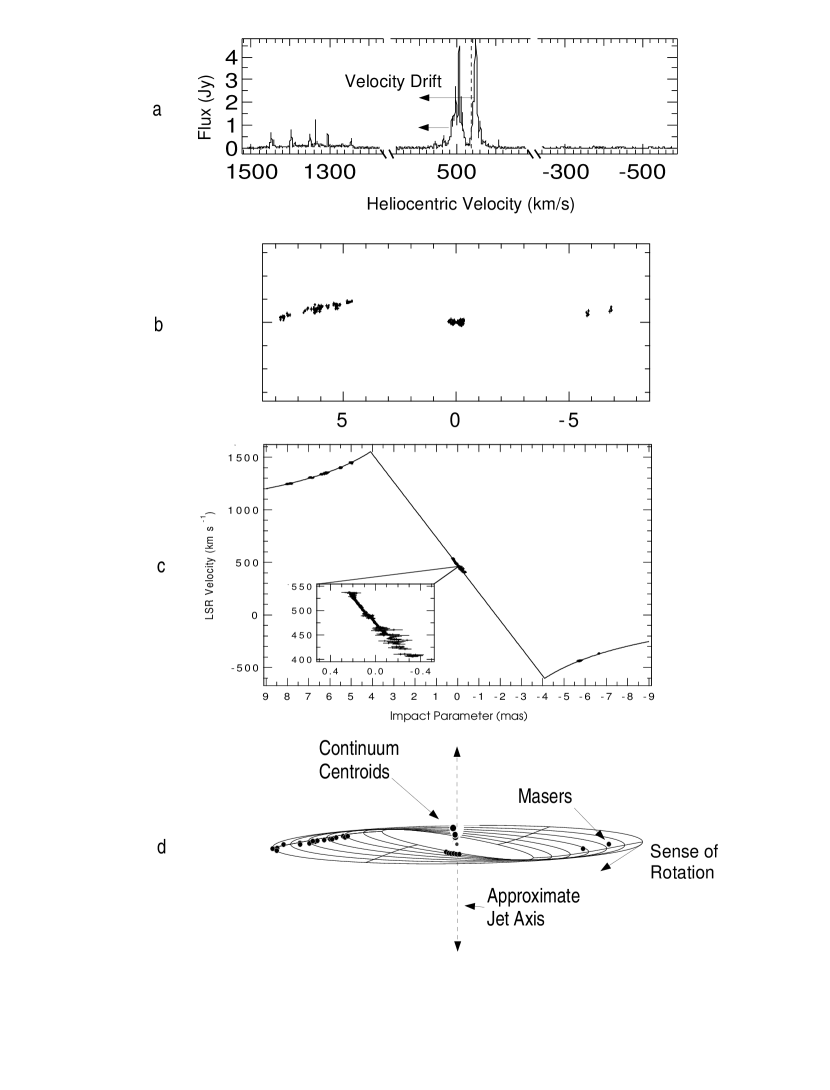
Figure 1:

Figure 2:

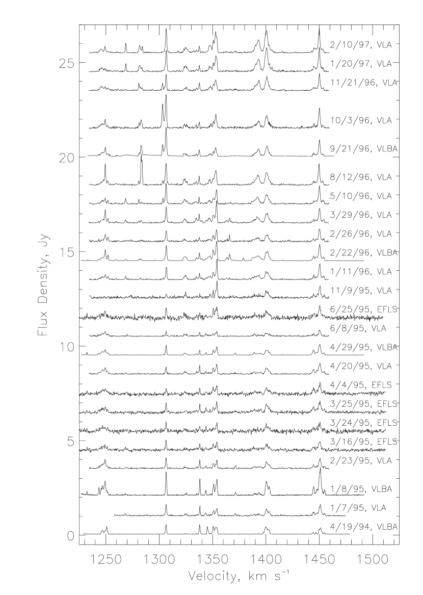
Figure 3:

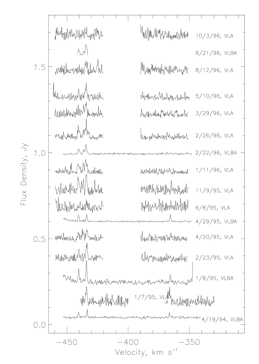
Figure 4:

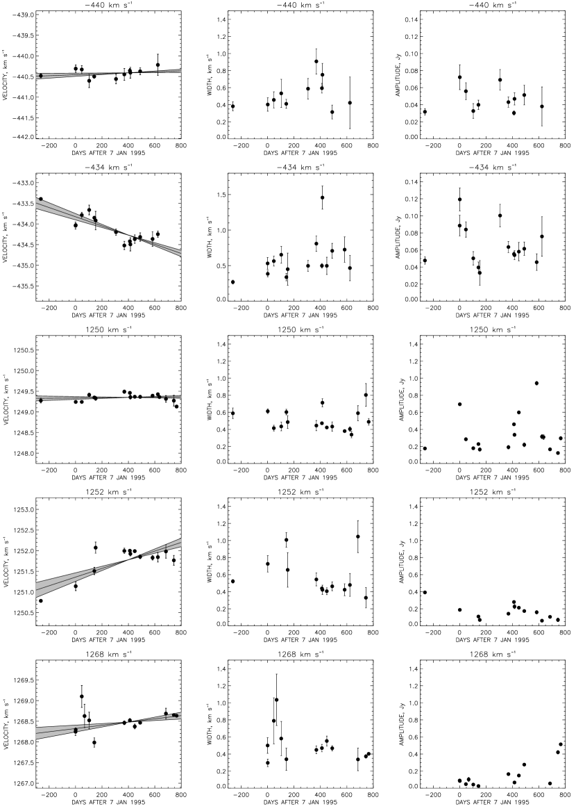
Figure 5a:

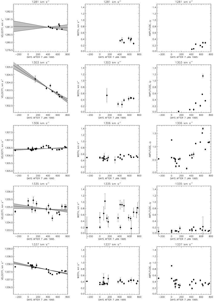
Figure 5b:

Figure 5c:

Figure 5d:

Figure 6:

Fig. 7. –

Fig. 8. –

Figure 9:

Figure 10:

Table 1: Summary of Observations

Date	Day	Telescope	Sensitivity	Comments
	Number		(mJy)
94 Apr 19	-263	VLBA	43	high-velocity emission only
95 Jan 7	0	VLA-CD	25	Velocity ranges shifted by +20 km s-1;
				1560 to 1635 km s-1 also observed
95 Jan 8	1	VLBA	80	high-velocity emission only
95 Feb 23	47	VLA-D	25
95 Mar 16	68	EFLS	85	redshifted emission only
95 Mar 24	76	EFLS	90	redshifted emission only
95 Mar 25	77	EFLS	95	redshifted emission only
95 Apr 4	87	EFLS	85	redshifted emission only
95 Apr 20	103	VLA-D	20
95 May 29	142	VLBA	30	high-velocity emission only
95 Jun 8	152	VLA-AD	20–35
95 Jun 25	169	EFLS	110	redshifted emission only
95 Jul 29	203	VLA-A	$\cdots$	no high velocity data calibration possible
95 Sept 9	245	VLA-AB	$\cdots$	no data calibration possible
95 Nov 9	306	VLA-B	37–60
96 Jan 11	369	VLA-BC	20
96 Feb 22	411	VLBA	25	high-velocity emission only
96 Feb 26	415	VLA-C	23–30
96 Mar 29	447	VLA-C	20
96 May 10	489	VLA-CD	15–24	-550 to -510 km s-1 and
				-330 to -290 km s-1 also observed
96 Jun 27	537	VLA-D	$\cdots$	thunderstorms – no useful data
96 Aug 12	583	VLA-D	23–36
96 Sept 21	623	VLBA	20	high-velocity emission only
96 Oct 3	635	VLA-AD	50
96 Nov 21	684	VLA-A	21–26	blueshifted velocities not observed
97 Jan 20	744	VLA-AB	27–37	blueshifted velocities not observed
				1475 to 1515 km s-1 observed
97 Feb 10	765	VLA-AB	17–23	blueshifted velocities not observed

Table 2: Measured Accelerations and Positions for High-velocity Features

Feature Velocity	Drift Rate	“Wobble Factor”	Angle off Midline	Radius
($\mathrm{km\ s^{-1}}$)	($\mathrm{km\ s^{-1}yr^{-1}}$)	$\sigma_{w}$ (km s-1)	(Degrees)	(Parsecs)
-440.4	+0.043 $\pm$ 0.036	0.021	+.0.6 $\pm$ 0.5	0.203
-434.3	-0.406 $\pm$ 0.070	0.152	.-5.6 $\pm$ 1.0	0.203
1249.4	+0.012 $\pm$ 0.031	0.084	+.0.3 $\pm$ 0.8	0.279
1251.8	+0.383 $\pm$ 0.095	0.220	+.9.3 $\pm$ 2.4	0.270
1268.5	+0.143 $\pm$ 0.076	0.180	+.3.3 $\pm$ 1.8	0.265
1281.0	-0.030 $\pm$ 0.184	0.098	.-0.7 $\pm$ 4.1	0.258
1303.7	-0.765 $\pm$ 0.115	0.062	-13.6 $\pm$ 2.3	0.230
1306.5	+0.041 $\pm$ 0.023	0.078	+.0.8 $\pm$ 0.4	0.242
1334.9	-0.104 $\pm$ 0.084	0.233	.-1.8 $\pm$ 1.4	0.226
1337.6	-0.237 $\pm$ 0.036	0.127	.-4.0 $\pm$ 0.6	0.224
1343.9	+0.299 $\pm$ 0.181	0.094	+.4.8 $\pm$ 3.0	0.220
1346.9	+0.232 $\pm$ 0.151	0.340	+.3.7 $\pm$ 2.4	0.219
1350.7	-0.010 $\pm$ 0.036	0.116	.-0.2 $\pm$ 0.6	0.218
1353.0	-0.084 $\pm$ 0.061	0.178	.-1.3 $\pm$ 1.0	0.217
1353.9	-0.023 $\pm$ 0.076	0.198	.-0.4 $\pm$ 1.2	0.217
1403.4	+0.141 $\pm$ 0.090	0.200	+.1.8 $\pm$ 1.1	0.194
1444.7	+0.190 $\pm$ 0.043	0.117	+.2.0 $\pm$ 0.5	0.178
1450.3	-0.331 $\pm$ 0.041	0.138	.-3.4 $\pm$ 0.4	0.176
1454.0	-0.745 $\pm$ 0.097	0.252	.-7.3 $\pm$ 1.0	0.172

Table 3: Measured Accelerations for Systemic-velocity Features

Feature Velocity (on Day 1)	Drift Rate	Error Estimate
($\mathrm{km\ s^{-1}}$)	($\mathrm{km\ s^{-1}yr^{-1}}$)	($\mathrm{km\ s^{-1}yr^{-1}}$)
423	8.02	1.40
460	9.29	0.13
464	9.39	0.22
480	9.31	0.14
483	10.40	0.20
490	10.18	0.13
496	8.96	0.14
500	9.37	0.13
504	9.54	0.20
506	9.50	0.25
515	8.17	0.18
530	7.47	1.64