ALTAI: Computational code for the simulations of TeV air showers as observed with the ground-based imaging atmospheric Čerenkov telescopes.

Abstract

Ground-based atmospheric Čerenkov telescopes are proven to be effective instruments for observations of very high energy (VHE) $\gamma$-radiation from celestial objects. For effective use of such technique one needs detailed Monte Carlo simulations of $\gamma$-ray- and proton/nuclei-induced air showers in Earth atmosphere. Here we discuss in detail the algorithms used in the numerical code ALTAI developed particularly for the simulations of Čerenkov light emission from air showers of energy below 50 TeV. The specific scheme of sampling the charged particle transport in the atmosphere allows the performance of very fast and accurate simulations used for interpretation of the VHE $\gamma$-ray observations.

1 Introduction

Recent exciting detections and observations of TeV $\gamma$-ray emission from a number of galactic and extragalactic objects (Ong 1998, Catanese & Weekes 1998) have shown the high performance of currently operating imaging air Čerenkov telescopes (IACTs). Several projects for future detectors have been proposed lately. The major forthcoming instruments, such as CANGAROO IV, H.E.S.S., MAGIC and VERITAS, will have significantly better sensitivity to $\gamma$-ray fluxes in the energy range from 50 GeV up to 50 TeV.

For a lack of a collimated test beam of TeV $\gamma$-ray photons, the ground-based Čerenkov detectors heavily rely on the Monte Carlo simulations of the Čerenkov light emission from air showers which are used to understand the performance of detector. Basic parameters of the instrument (detection area, angular and energy resolution, efficiency of cosmic ray rejection, etc) can be derived from the simulations. The crucial point is a precise measurement of the primary shower energy. For that one should include properly into the simulations all processes of Čerenkov light emission in the air shower as well as photon propagation on the way from the emitting shower particle to the telescope camera. Measurements of $\gamma$-ray fluxes, energy spectra, upper limits strongly depend on the absolute energy calibration of a telescope.

Here we give a description of ALTAI computational code developed for detailed Monte Carlo simulations of the Čerenkov light emission in TeV air showers. Among the other existing codes intended for such simulations, MOCCA (Hillas 1979), KASCADE (Kertzman & Sembroski 1994), CORSIKA (Heck et al. 1997), this code has a distinctive advantage – it’s rather high speed of shower simulations due to a specific algorithm used for processing the multiple scattering of charged shower particles. This approach does not consume a lot of CPU time and allows to perform fast and accurate simulations. Together with the additional routine recently developed for the simulations of telescope response (Hemberger 1998) the ALTAI code was extensively used for production of a standard Monte Carlo database used in the HEGRA (High Energy Gamma Ray Astronomy) VHE $\gamma$-ray experiment (Konopelko et al. 1999a).

The ALTAI code consists of two major programs which simulate the development of the electromagnetic (EMCCS) (hereafter we put in brackets the name of the corresponding subroutine of the code) and proton-nuclei (STEPAD, MULTIP, XPI) cascade in Earth atmosphere. We discuss in detail the procedure of simulating the electromagnetic and hadron-nuclei cascade in Sections 2 and 3, respectively. Section 2 also describes the algorithms of Čerenkov light emission by the shower charged particle. Section 4 deals with nucleus-nucleus interactions. In Section 5 we review the results of the Čerenkov light simulations using ALTAI code compared with other relevant simulations and observational data.

Figure 1: Transformation of phase coordinates of a charged particle at the multiple scattering segment.

2 Electromagnetic cascade

Here we overview the part of the code intended for the generation of an electromagnetic cascade in the atmosphere (EMCCS). Note that at present all cross-sections for electron and photon interactions are established and are well described in detail in the relevant energy range. An electromagnetic part of the code accounts for the following interaction processes: electron-positron pair production, Compton scattering for the primary photons and bremsstrahlung, ionization losses, Coulomb scattering for the primary electrons and positrons.

The cross-section of $e^{-},e^{+}$ pair production by primary photon was calculated according to the Bethe-Heitler formula taken from Motz et al. (1964) (MPRH). The emission angle of $e^{-},e^{+}$ components, defined with respect to the direction of initial photon, was sampled using the Bethe distribution (Motz et al. 1964). We used the Klein-Nishina formula (see e.g., Gaisser 1990) for the cross-section of Compton photon scattering (COMPH). The dependence of photon cross-sections on energy and the atomic number of a medium was derived from data taken from Storm & Israel (1973) and Hubbel (1969) (FMPM).

We simulated the bremsstrahlung interaction process (MRDH) according to the Bethe-Heitler formula (see Koch & Motz, 1959). The angle of emitted photon was sampled from the Schieff distribution (see Koch & Motz, 1959). The Bethe-Bloch formula, with the corrections for the density effect (Sternheimer 1952), was used for simulation of the mean ionization losses (MIONH) whereas for the differential cross-section of $e^{-},e^{+}$ ionization collisions we used the Möller formula (Möller 1932). Note that in the electromagnetic shower positrons were treated similarly to electrons.

2.1 Multiple scattering

The relativistic electron suffers an enormous number of interactions along its path length in the matter. Apparently, a direct simulation of all interactions is not possible. That is why all numerical codes for the shower simulation use a specific technique for grouping electron interactions (see for review Berger 1963, Akkerman 1991, Gaisser 1990). In this approach one can simulate only the so-called catastrophic $e^{-},e^{+}$ interactions. These interactions lead to emission of photon/electron of a relatively high energy, $\rm E>Q$, which exceeds the intermediate energy threshold of $\rm Q$. The same approach was used for the simulation of the $e^{-},e^{+}$ ionization process ($\rm Q=Q_{I}$) and bremsstrahlung ($\rm Q=Q_{R}$). The emitted electron must have a kinetic energy above a certain intermediate energy threshold, $\rm T>Q_{I}$.

A random path length between neighboring catastrophic collisions was divided into small segments of $\rm\Delta l\leq 5\,gr/cm^{2}$. We sampled the phase coordinates of a charged particle at the end of the segment $\rm\Delta l$ according to the cumulative effect of all low energy collisions along the segment (SGMEH, SGMQH). Thus we simulated at the end of each segment the loss of the $e^{-},e^{+}$ kinetic energy, $\rm\Delta T=T_{1}-T_{2}$, the scattering angle, $\rm\Theta=\arccos(\vec{\Omega}_{1}\vec{\Omega}_{2})$, the azimuth angle of scattered particle, $\rm\varphi$, the longitudinal $\rm Z$ and lateral $\rm\vec{\rho}$ displacement of initial particle while passing over the segment (see Figure 1). Appropriate transport equations were used in order to derive the probability distributions for the phase coordinates at the end of a segment. We have obtained the analytical solutions for these distributions.

2.1.1 Energy losses

The energy losses of a charged particle, $\rm\Delta E$, in the segment, $\rm\Delta l$, were sampled according to the Landau-Vavilov formula (Landau 1944, Vavilov 1957). Plyasheshnikov & Kolchuzkin (1975) have tabulated this formula for a specific conditions of shower simulations. The distribution of the energy losses at the end of a multiple-scattering segment was described as follows:

$$P(\Delta T)d\Delta T=f(\mu,\lambda)d\lambda,$$

$$f(\mu,\lambda)=\frac{1}{2\pi i}\int_{c-i\infty}^{c+i\infty}\exp\left\{\lambda t-\mu\phi(t)\right\}dt,$$

$$\phi(t)=t\int^{t}_{0}\frac{(1-\tau-exp(-\tau))}{\tau^{2}}d\tau$$

$$\mu=\Sigma_{h}(T_{1})\Delta l,$$

$$\lambda=(\Delta T-\beta_{l}(T_{1})\Delta l)/Q_{I},$$

$$\Sigma_{h}(T)=\int_{Q_{I}}^{T/2}W_{I}(T,Q)dQ,$$ (1)

where

$$\beta_{l}(T)=\beta_{I}+\beta_{R}$$

$$\beta_{I}=\int_{0}^{Q_{I}}W_{I}(T,Q)QdQ$$

$$\beta_{R}=\int_{0}^{Q_{R}}W_{R}(T,Q)QdQ$$ (2)

is the mean energy loss per unit path length due to the inelastic collisions of a charged particle by production of low energy secondaries. $\rm W_{I}(Q),W_{R}(Q)$ are the differential cross-sections for the ionization ($\rm I$) and bremsstrahlung ($\rm R$) interactions.

The standard inverse function technique was applied in order to simulate the energy loss $\Delta T$ according to the two-dimensional distribution $f(\mu,\lambda)$ (Eqn. (1)). For that one needs to compute the tables of the function $\tilde{\lambda}=\tilde{\lambda}(\mu,\alpha)$, which is inverse to the integral distribution

$$F(\mu,\lambda)=\int_{-\infty}^{\lambda}f({\mu,\tilde{\lambda}})d\tilde{\lambda}$$ (3)

These tables can be found, e.g., in Akimov et.al. (1981) where $\tilde{\lambda}=\tilde{\lambda}(\mu,\alpha)$ was tabulated over a two-dimensional lattice with the steps of 0.025 and 0.01 over $\alpha$ and $\mu$, respectively. First, it is necessary to generate the random number $\alpha$ uniformly distributed in the interval (0,1) and calculate parameter $\mu$ according to Eqn. (1). After that one should interpolate $\lambda=\lambda(\mu,\alpha)$ using the above mentioned tables and finally determine $\Delta T$ as

$$\Delta T=\beta_{I}\Delta l+\lambda Q_{I}$$ (4)

where

$$\lambda=\left\{\begin{array}[]{l}\mu^{1/2}\cdot\tilde{\lambda},\quad\mu<0.1;\\ \mu\cdot(\tilde{\lambda}+\ln\mu),\quad\mu\geq 0.1\end{array}\right.$$ (7)

Formula (5) was derived using two asymptotics of initial distribution (1) for $\mu=0$ and $\mu=\infty$, which were sewn up at $\mu=0.1$. The subroutine ELSH makes calculations according to these algorithms.

2.1.2 Angular deflection

We simulated the angle of multiple scattering using the Moliere theory (Moliere 1948, Bethe 1953). In addition we have improved the Moliere distribution by taking into account the energy losses at the multiple scattering segment. This distribution may be described as follows:

$$P(\Theta)\Theta d\Theta=\left[f_{0}(\tilde{\Theta})+\frac{f_{1}(\tilde{\Theta})}{B}+\frac{f_{2}(\tilde{\Theta})}{B^{2}}\right]\tilde{\Theta}d\tilde{\Theta},$$ (8)

where

$$\tilde{\Theta}^{2}=\frac{\Theta^{2}}{\tilde{\chi}_{c}^{2}}\cdot B,$$

$$\tilde{\chi}_{c}^{2}=\int_{T_{o}}^{T_{1}}\chi_{c}^{2}(T)/\beta_{l}(T)dT,$$

$$T_{o}=T_{1}-\beta_{l}(T_{1})\Delta l.$$ (9)

Parameter $\rm B$ was determined by resolving the transcendental equation $B-\ln B=\ln(0.856(\tilde{\chi}_{c}/\chi_{a})^{2})$. Functions $f_{n}(n=0,1,2)$ were calculated as

$$f_{n}(\tilde{\Theta})=\int_{0}^{\infty}(\frac{u^{2}lnu}{4})^{n}e^{-\frac{u^{2}}{4}}J_{o}(\tilde{\Theta}u)udu.$$ (10)

Quantities $\chi_{c}$ and $\chi_{a}$ are closely related to the differential cross-section for Coulomb scattering (see formula (10) for definition of the Coulomb cross-section).

For a fixed segment length $\rm\Delta l$ and kinetic energy of a particle $\rm T$ one can determine in a few iterations the parameter $\rm B$, which defines the shape of the distribution $\rm P(\Theta)$. Such calculations were done by use of subroutine ANGMH.

2.1.3 Space displacement

At the multiple scattering segments we simulated the longitudinal displacement $\rm Z$ of a charged particle. For that we used the Yang-Spenser distribution (Yang 1951, Spencer & Coune 1962). This distribution was adapted for the air shower simulations by Plyasheshnikov & Kolchuzhkin (1975). This distribution may be represented by the following expression

$$P(Z)dZ=-e^{\nu}f(\nu,\xi)d\xi$$

$$f(\nu,\xi)=\frac{1}{2\pi i}\int_{c-i\infty}^{c+i\infty}u^{1/2}cosch(u^{1/2})e^{q}du$$

$$q=\xi u-\nu u^{1/2}ctg(u^{1/2}),$$ (11)

where

$$\nu=\frac{1-cos\Theta}{\eta\Delta l},\,\,\xi=\frac{\Delta l-Z}{\eta\Delta l^{2}},$$

$$\eta=2\pi\int_{-1}^{+1}W_{c}(T_{1},\theta)(1-cos\theta)d\cos\theta$$

$$W_{c}(T,\theta)=2\chi_{c}^{2}/(\theta^{2}+\chi_{a}^{2})^{2}.$$ (12)

Here $\rm W_{c}(T,\theta)$ is a cross-section of the Coulomb scattering which determines parameters $\rm\chi_{a}$ and $\chi_{c}$.

To simulate the longitudinal displacement $Z$ we use approach similar to that used in Section 2.1.1 for simulation of the energy loss $\Delta T$. It is based on the interpolation of the two-dimensional function $\xi=\xi(\nu,\alpha)$, which is the inverse function to the integral distribution

$$F(\nu,\xi)=\int_{0}^{\xi}f(\nu,\tilde{\xi})d\tilde{\xi}$$ (13)

One can find these tables, e.g., in Akimov et.al (1981). This approach includes (i) sampling of the random number $\alpha$, (ii) calculation of $\nu$ on the basis of quantities $T_{1}$ and $\Delta l$, (iii) determination of $\xi$ on the basis of the two-dimensional interpolation using the above mentioned tables and, finally, calculation of $Z$ according to the formula

$$Z=\Delta l-\xi\eta\Delta l^{2}.$$ (14)

For the lateral displacement of a charged particles at the multiple scattering segment we defined the corresponding probability distribution using Fermi formula (see e.g., Kolchuzhkin & Plyasheshnikov 1975). This distribution was derived by solving the transport equations in the Focker-Planck approximation where the collision integral corresponding to the Coulomb scattering was replaced by a second order differential operator (see e.g., Kolchuzhkin & Uchaikin 1978). For the fixed angle of multiple-scattering $\vec{\Theta}=$ $(\Theta_{x},\Theta_{y})=$ $(\Theta\cos\varphi,\Theta\sin\varphi)$ this distribution was as follows

$$P(\vec{\psi})=\frac{6}{\pi\gamma}\exp\left[-\frac{6}{\gamma}(\vec{\psi}-\vec{\Theta}/2)^{2}\right],$$

$$\vec{\psi}=\vec{\rho}/\Delta l,$$ (15)

where the parameter $\gamma=\eta\Delta l$ defines the width of the distribution. As was shown by Kolchuzhkin & Plyasheshnikov (1975) more accurate numerical solution of the transport equations reduces by a factor of 1.5 the width of the final distribution. This difference may be corrected by introducing another definition for the parameter $\gamma$:

$$\gamma=\chi_{c}^{2}\cdot\tilde{B}.$$ (16)

where $\rm\tilde{B}$ is determined from $\tilde{B}-ln\tilde{B}=ln((\tilde{\chi}_{c}/\chi_{a})^{2}/1.80)$. The complete procedure for charged particle transport in multi-dimensional phase space of energy, angular and space coordinates was defined by a few parameters: two threshold energies $\rm Q_{I}$, $\rm Q_{R}$, and the length of a multiple-scattering segment $\rm\Delta l$. The extensive test calculations using the ALTAI code revealed the optimum values of parameters which allow to perform rather fast shower simulations without introducing systematic errors. Thus we used the following parameters for the calculational procedure: $\rm Q_{I}\simeq 0.5\,T_{o}$, $\rm Q_{R}\simeq 0.1\,T_{o}$, where $\rm T_{o}\simeq 20$ MeV is the threshold energy for Čerenkov light emission by cascade electrons in air.

Apparently the length of a multiple scattering segment, $\rm\Delta l$, is one of the basic parameters of this method. By use of rather small segments one can reduce systematic error introduced by approximations of analytical solutions for the phase transformations at the multiple scattering segment. On the other hand this may slow down the procedure of shower simulation. We found that the optimum length of the multiple-scattering segment is within the range of $\rm\sim 1-5\,gr/cm^{2}$. Very accurate analytical solutions of a multiple-scattering process for a $e^{-},e^{+}$ transport allow us to use in calculations such segment length without introducing systematic errors in three-dimensional shower development.

In comparison to other computational codes we used more accurate distributions derived analytically from the multiple scattering theory. On the contrary the standard approach used for example in EGS-IV code does not include fluctuations of the energy losses at the multiple-scattering segment. In addition, in the EGS-IV code the lateral displacement of charged particle at the multiple-scattering segment is taken as $\vec{\rho}=0$ and correspondingly the longitudinal displacement is of $z=\Delta l$. All this necessitates a small segment length and makes significantly more time consuming the shower simulations. Thus for the simulations of Čerenkov light from the TeV air shower ALTAI code is faster by as much as a few times compared with the EGS-IV.

2.2 Emission of Čerenkov Light

A charged particle ($e,\mu$) in an air shower can emit Čerenkov light when its energy exceeds a certain threshold energy $\rm E>E_{th}$. The threshold energy is determined as (Frank & Tamm 1937)

$$E_{th}=\frac{m_{o}c^{2}}{\sqrt{2(n-1)}}$$ (17)

where $\rm n$ is the refraction index in air, $\rm m_{o}$ is the particle mass. Thus at sea level the energy threshold is $E_{th}\simeq$20 MeV for electron and $\simeq$4 GeV for muons. To describe the altitude dependence of the refraction index we used the following expression (Beliaev et al. 1980)

$$n=1+\eta,\quad\eta(H)=\eta_{o}/\rho_{o}\cdot\rho(H)$$ (18)

where $\eta_{o}=2.9\cdot 10^{-4}$, $\rho_{o}=1.22\cdot 10^{-3}\,\rm g/cm^{3}$, and $\rho(H)$ is the air density at a height H above the sea. The model of a standard atmosphere (Elterman 1968) was used in the simulations.

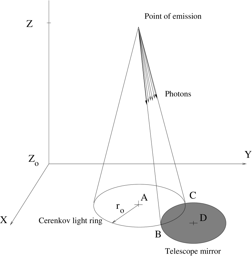
Figure 2: Geometry of propagation of Čerenkov light photons.

According to Frank & Tamm (1937) the mean number of Čerenkon photons emitted in a 1 cm pathlength by electron is described as

$$\frac{dQ}{dl}=2\pi\alpha(\frac{1}{\lambda_{1}}-\frac{1}{\lambda_{2}})\sin^{2}\theta_{c}$$

$$\sin^{2}\theta_{c}=1-\frac{1}{(1-(mc^{2}/E)^{2})n^{2}}$$ (19)

where $\alpha$ is a fine structure constant $\alpha=1/137$ and $\theta_{c}\simeq 1^{o}$ is the opening angle of the Čerenkov light cone. The spectral region of emission is defined by wavelengths $\lambda_{1}$ and $\lambda_{2}$. In simulations we included sampling of the Čerenkov light attenuation in the atmosphere due to the Raleigh scattering, ozone and aerosol absorption. The cross-sections for these processes were calculated using the data of Driscoll & Vaughan (1978).

In the shower simulation procedure (PARCHR, GSTCHR) (Konopelko 1990), we first define the total number of Čerenkov photons $\rm<n_{ph}>$ emitted at the multiple scattering segment $\rm\Delta l$. As was discussed above we used rather small multiple scattering segments. Therefore, we can assume that all Čerenkov photons are emitted from the center of the multiple scattering segment (see Figure 1). To a rather good approximation an intersection of the Čerenkov light cone with the observation plane forms a circle of a radius $\rm r_{c}$ which can be calculated as

$$r_{c}=(Z-Z_{obs})\cdot\theta_{c}$$ (20)

where $Z$ and $Z_{obs}$ are the height of Čerenkov light emission and the height of the observation level above the sea, respectively. The number of photons hitting the telescope mirror can be calculated as

$$<\tilde{n}_{ph}>=\frac{\Delta L}{2\pi r_{c}}(1-p(Z,Z_{obz}))<n_{ph}>$$ (21)

where $\Delta L$ is length of the circle arc between points B and C (see Figure 2). $\rm p(Z,Z_{obs})$ is a probability of the Čerenkov light attenuation in the atmosphere along the way of a photon propagation. For specific response functions of the telescope camera one may calculate corresponding average number of photoelectrons as $\rm<n_{ph.e.}>=\xi<\tilde{n}_{ph}>$, where $\xi$ is a photon-to-photoelectrons conversion efficiency. Finally one can use the Poisson distribution in order to simulate the random number of photons (photoelectrons) hitting the telescope. The photons reaching the telescope mirror were uniformly distributed over the circle arc BC (see Figure 2).

In the latest version of the ALTAI code we save all, or a certain fraction, of Čerenkov photons hitting the telescope. Each photon has a set of 6 variables, $\vec{\upsilon}(x,y,\theta_{x},\theta_{y},z_{o},t)$. $\rm z_{o}$ is a height of the photon emission (in $\rm g/cm^{2}$) and $t$ is a time of photon arrival to the detector. Such database of the photon is used for detailed simulations of the telescope camera response (Hemberger 1998).

Table 1: Mean number of fragments created by different nuclei (Murzin 1988).

Primaries $\mid$ Secondaries	$Z>10$	C,N,O,F	Li, Be, B	He
$Z>10$	0.17	0.29	0.26	1.34
C,N,O,F	–	0.11	0.24	1.00
Li,Be,B	–	–	0.15	0.51

3 Hadron-nuclei cascade

For simulations of the hadron-nuclei cascade we used the phenomenological model of hadron interactions (Konopelko 1990) which, in the most part, is based on the available accelerator data. The energy spectra of secondary hadrons generated in a $pA$ interactions were approximated by use of the radial scaling model (Hillas 1979). In this approach the energy spectra may be presented as

$$xdN/dx=F_{(p\rightarrow q)}(x)H_{q}(x,E),x=E/E_{o}$$ (22)

where $E_{o},E$ are the energies of the primary and secondary particles, respectively. Indeces $p,q$ denote the type of primary and secondary particle ($p,n,\pi^{+},\pi^{-},\pi^{o}$). The basic functions are given below

$$F_{(p,n)\rightarrow\pi^{\pm}}=$$

$$F_{(p,n)\rightarrow\pi^{0}}=$$

$$1.22(1-x)^{3.5}+0.98e^{-18x},$$

$$F_{\pi^{\pm}\rightarrow\pi^{0}}=1.3(1+\frac{x}{0.45})^{-3},$$

$$F_{\pi^{\pm}\rightarrow\pi^{\pm}}=F_{\pi^{\pm}\rightarrow\pi^{0}}+0.57e^{4(x-1)},$$

$$H_{(p,n)\rightarrow(\pi^{\pm},\pi^{o})}=[1+\frac{0.4}{E+0.14}]^{-1},$$

$$H_{\pi^{\pm}\rightarrow(\pi^{\pm}\pi^{o})}=1-0.88e^{-1.8x}$$ (23)

For the total cross-sections of inelastic hadron interactions we used the data given by Shabelski (1986,1987) in the following form

$$\sigma_{\pi^{\pm}}=1.2\sigma_{(p,n)},$$

$$\sigma_{(p,n)}=\left\{\begin{array}[]{l}258\,\,E<E_{1},\\ 273(1+3.29\cdot 10^{-2}y+\\ 3.88\cdot 10^{-3}y^{2})\,\,E_{1}<E<E_{2},\\ 258(1+0.07y)\,\,E>E_{2}\\ \end{array}\right.$$ (28)

$$E_{1}=100\,GeV,E_{2}=10^{4}\,GeV,$$

$$y=ln(E/10^{3}\,GeV)$$ (29)

The cross-sections from Eqn. (22) are measured in mBarn and correspond to the particle interaction with air. We assume that the mean value of atomic number for air nuclei is of 14.4.

We used a simplified geometrical representation (Murzin 1988) for the total cross-section of the nucleus-nucleus interactions as follows

$$\sigma_{A}=R^{2}\sigma_{N},$$

$$R=\frac{A^{1/3}+A_{0}^{1/3}-b}{1+A_{0}^{1/3}-b},$$ (30)

where $A_{0}$ is the effective atomic mass of air ($A_{o}=14.4$) and $b$ is the effective radius of nuclei overlapping zone ($b=1.17$). $\sigma_{N}$ defines the cross-section of hadron interaction with air.

The transverse momenta of secondary hadrons were calculated according to the distribution given by Ranft (1972)

$$f_{(p,n,\pi^{\pm})}(p_{\perp})=p_{\perp}\frac{e^{-Bp_{\perp}^{2}}+Ce^{-Dp_{\perp}}}{\frac{1}{2D}+\frac{C}{D^{2}}}$$ (31)

where the corresponding parameters (B,C,D) were defined for the interactions with air as described by Ranft et al. (1972). $p_{\perp}$ is measured in GeV/c.

The ALTAI code was developed for the simulations in the energy range relevant for the very high energy $\gamma$-ray astronomy $\rm E\leq 50\,TeV$. In this energy range the mean number of kaons ($\rm K^{\pm},K^{o}$) produced in hadron-nuclei interactions is very small compared with the number of emitted pions ($\rm\pi^{\pm},\pi^{o}$). Besides this, in this energy region kaons and pions exhibit similar properties of inelastic interactions (see, e.g., Grishin 1982). Thus in the shower simulations for this restricted energy range we can exclude the kaon production process by introducing appropriate corrections for the probabilities of pion production in the $(p,n,\pi^{\pm})\rightarrow X$ inelastic collisions.

For each inelastic hadron interaction (MULTIP) we sampled first the energy of the so-called leading particle ($p,n,\pi^{\pm}$). This particle carries away the bulk of the primary energy. We assume that the energy of a leading particle E is uniformly distributed within the range $(0,E_{0})$ where $E_{0}$ is the energy of a primary interacting particle. Note that the type of the leading particle was selected randomly amongst proton and neutron for interaction $(p,n)+A\rightarrow(p,n)$, and amongst charged pion or neutral pion for interaction $(\pi^{\pm},\pi^{o})+A\rightarrow(\pi^{\pm},\pi^{o})$. Thus the total inelasticity coefficient was determined as $\kappa=1-E/E_{0}$. At the next step we sampled multiple production of other secondary particles ($\pi^{\pm},\pi^{o}$). The type of secondary particle was randomized assuming that $\pi^{o}$ pions forms, on average, one third of all pions generated in hadron interactions. The energy of secondary particle was simulated using the spectra given by Eqn. (22). We have completed the production of secondary particles when their total energy exceeds the energy of a primary particle. The energy of the last simulated particle was renormalized in order to conserve the total energy in each inelastic interaction.

The transverse momentum of the secondaries was simulated using Eqn. (31). By the renormalization of the transverse momentum of leading particles we allowed to fulfill the momentum conservation for each hadron interaction without distortion of stochastic properties of a multi-particle production process. The test calculations have shown that such an approach describes very well the initial inclusive spectra of the secondary particles if the number of secondaries is relatively high ($\gg 1$). Note that as almost identical algorithm was developed and tested by Barashenkov & Toneev (1972).

Note that we have included in the code the propagation of a single muon generated in the hadron-nuclei cascade due to the $\pi^{\pm}$ decay (SGG,TRMUON). The emission of the Čerenkov light from the muons was included in simulations according to the scheme described above.

4 Nucleus-nucleus interactions

We have implemented in the ALTAI code a model of independent nucleon interactions of colliding nuclei with nuclei fragmentation included (TAFRAC, TRAN, FRAG, OVERLAP). In this approach we assume that all nucleons of the projectile nucleus have the same energy determined as $E_{0}/A_{p}$. $E_{0}$ and $A_{p}$ are the energy and atomic number of projectile nucleus, respectively. All nucleons of the projectile nucleus which overlap with the target nucleus interacted independently with each other. The non-overlapping part of the projectile nucleus decayed into individual nucleons and heavier fragments. The energy of fragment with the atomic number $A$ is defined as $E_{f}=(E_{0}\cdot A)/A_{p}$. We simulated a random number of a fragments according to the probabilities of different channels summarized in Table 1.

5 Comparison with other codes and data

An overview of Monte Carlo results on lateral, temporal, and angular characteristics of the Čerenkov light in air showers of 10 GeV - 1 TeV was recently given by Konopelko (1997). Most of the Čerenkov light characteristics calculated with the ALTAI code reproduce rather well the results obtained with the MOCCA code (Hillas 1996). The stereoscopic observations of BL Lac object Mkn 501 in 1997 with the HEGRA system of imaging air Čerenkov telescopes allowed the first measurements of the parameters of the Čerenkov light images from the $\gamma$-ray-induced air showers. The HEGRA data are in excellent agreement with the results of Monte Carlo simulations obtained with ALTAI code (Aharonian et al. 1999a). Using the Mkn 501 data sample comprising 38,000 $\gamma$-ray events we have tested in great detail the parameters of Čerenkov light image orientation and shape (Konopelko et al. 1999a) (see Figure 3) as predicted by the simulations.

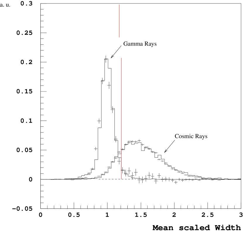
Figure 3: Distribution of a shape parameter (mean scaled Width) of Čerenkov light images simulated with ALTAI code (histograms) and recorded with HEGRA system of IACTs (crosses).

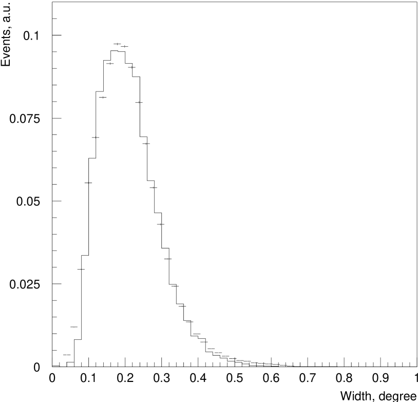
Figure 4: Distribution of image shape parameter Width for the ALTAI simulated events (histogram) and cosmic ray images recorded with a 10 m Whipple IACT (crosses) (Konopelko 1999b).

The HEGRA stereoscopic system of 5 IACTs was used for the measurements of the lateral distribution of the Čerenkov light in the $\gamma$-ray-induced air showers. These measurements have been compared again with the Monte Carlo simulations using the ALTAI code (Aharonian et al. (1998)). The simulations using the ALTAI code reproduce very well the measured lateral distributions of the Čerenkov light. Note that the measured shape of the Čerenkov light lateral distributions is almost independent of the detector simulation procedure but strongly depends on the development in space of a multi-TeV $\gamma$-ray shower in the atmosphere.

We made several comparisons of the shape and size (total number of photoelectrons) of the Čerenkov light images for the proton- and nuclei-induced air shower calculated with the ALTAI and CORSIKA codes (Heck et al. 1997). The CORSIKA code was used with the HDPM model of the proton-nuclei interactions. This model is based on supercollider data and describes rather well the proton-nuclei air showers of energy below 10 TeV. In addition, the HDPM model of CORSIKA allows to perform relatively fast calculations with respect to other more modern shower generators, e.g. VENUS/QGSJET. Despite the different algorithms and schemes in the two codes the results appeared to be almost identical (Plyasheshnikov et al. 1997). The simulations with the ALTAI and CORSIKA codes well reproduce each other. Note that simulations with the ALTAI code are essentially less time consuming. The HEGRA data for the cosmic ray air showers were compared with the ALTAI simulations. Good agreement between simulations and data provided a precise measurement of the cosmic ray proton spectrum in the energy range $\sim$1-5 TeV (Aharonian et al. 1999b).

We show in Figure 3 the distribution of so-called mean scaled Width parameter for primary $\gamma$-rays and cosmic rays extracted from the HEGRA data as well as from the Monte Carlo simulations. The simulations fit very well the data. Recently, we compared the relevant results of the ALTAI simulations with the cosmic ray data taken with a 10 m Whipple imaging air Čerenkov telescope during the 1995/1996 Crab Nebula observations (Konopelko 1999b). For these simulations we have used the standard detector response functions offered by the Whipple collaboration. The simulations reproduced very well the shape of recorded Čerenkov light images (see Figure 4).

As mentioned above the upper energy of the shower simulations is about 50 TeV. It is limited by the simplified phenomenological model of the hadronic cascade. Although in the case of pure electromagnetic showers one can extend simulations using the ALTAI code to much higher energies without breaking any model restrictions such extension may need the introduction of a number of changes into the code for the correct treatment of a larger number of particles.

6 Summary

Here we have presented a detailed description of the numeric code ALTAI, which was developed for simulations of Čerenkov light from extensive air showers. This code allows to make very fast and accurate calculations of the response of the ground-based Čerenkov detectors used in VHE $\gamma$-ray astronomy. Although the code was designed for calculating the parameters and characteristics of the imaging air Čerenkov telescopes it can be rearranged with minor changes in order to simulate the responses of showerfront sampling experiments like MILAGRO, or Tibet AS-$\gamma$.

We tested our computational code against the data taken with two currently operating detectors, the HEGRA system of imaging air Čerenkov telescopes and the state-of-the-art single 10 m Whipple telescope. These comparisons have proven the high precision of the simulations. The computational code ALTAI is an effective tool for producing the simulated data for VHE $\gamma$-ray astronomy. Note that the forthcoming imaging Čerenkov detectors (CANGAROO IV, H.E.S.S., MAGIC, VERITAS) will need a large amount of simulated data. Therefore the performance of these instruments may benefit from the use of the ALTAI code.

7 Acknowledgments

The work for the ALTAI code was primarily initiated and substantially advanced at the Tomsk Technological University, Tomsk, Russia, where the major algorithms of the shower simulation scheme were developed. Authors thank Prof. A.M. Kolchuzhkin for a significant contribution for all these studies. In the most part the ALTAI code was developed and programmed at the Altai State University, Barnaul, Russia. The authors thank Dr K.V. Vorobjev, Prof A.M. Lagutin, Dr V.A. Litvinov and Prof V.V. Uchaikin for their valuable input and support of this activity. The computational code ALTAI was used and further developed at the Max-Planck-Institut für Kernphysik, Heidelberg. The authors would like to acknowledge the contribution and support of all members of the Heidelberg group in particular Prof F. Aharonian, Dr M. Hemberger, Prof W. Hofmann, J. Kettler and Prof H.J. Völk. AKK thanks Prof T.C. Weekes for support and supervision of a short-term project at the University of Arizona, Tucson, and at the Whipple Observatory, Harvard-Smithsonian Center for Astrophysics, Amado.

We are grateful to an anonymous referee for detailed and helpful comments.

8 Availability

The ALTAI code is written in FORTRAN and may be easily installed at any computer platforms maintaining FORTRAN compiler. Regarding the availability of the code contact: alexander.konopelko@mpg.mpi-hd.de

References

- [1] Aharonain F., et al. (HEGRA Collaboration) Astropart. Phys., 10, 21 (1998).
- [2] Aharonian F., et al. (HEGRA Collaboration) Astron. Astrophys. 349, 11 (1999a).
- [3] Aharonian F., et al. (HEGRA Collaboration) Phys. Rev. D 59, 9, 2003 (1999b)
- [4] Akimov B.B., et al. Institute of Space Research, Russia Academy of Science, Preprint N684 (1981).
- [5] Akkerman A.F. Simulation of trajectories of charged particles in the matter, Energoatomizdat, Moscow (1991).
- [6] Barashenkov V.S., Toneev V.D. Interactions of High Energy Particles with Atomic Nuclei (in Russian), Atomizdat, Moscow (1972).
- [7] Beliaev A.A., Ivanenko I.P., Kanevsky B.L. et al. Electromagnetic cascades in cosmic rays at very high energies (in Russian), Nauka, Moscow (1980).
- [8] Berger M.J. in: Methods in computational physics. New York- London Academic Press, 1, 135 (1963).
- [9] Bethe H.A. Phys. Rev. 89, 6, 1256 (1953)
- [10] Catanese M., Weekes T.C. Publ. Astron. Soc. Pac., 111, 1193 (1999).
- [11] Driscoll W.G., Vaughau W., Handbook of Optics, McGraw-Hill Book Company (1978)
- [12] Elterman L. Air Force Cambridge Res. Lab. Rep. 40, AFC RL-68-153 (1968)
- [13] Frank I.M., Tamm I.E. Theory of Vavilov-Čerenkov radiation, Bull of Acad. of Science USSR, 14, 109 (1937).
- [14] Gaisser T. Cosmic rays and particle physics, Cambridge University Press (1990).
- [15] Grishin V.G. Inclusive Processes in Hadron Interactions at Very High Energies (in Russian), Atomizdat, Moscow (1982).
- [16] Heck D. et al. Proc. IXth Int. Symp. on VHE Cos. Ray Interactions, Karlsruhe (eds. Rebel H., Schatz G., Knapp J.), Nucl. Phys. B (Proc. Suppl.) 52B, 139 (1997).
- [17] Hemberger M., PhD thesis, University of Heidelberg (1998).
- [18] Hillas A.M. Proc. of 16th ICRC, Kyoto, v.6, 13 (1979).
- [19] Hillas A.M. Space Sci. Rev. 75, 17 (1996).
- [20] Hubbel J.H. Photon cross-sections, attenuation coefficients and energy absorption coefficients from 10 KeV to 100 GeV, NSRDS-NBS29, Washington (1969).
- [21] Kertzman M.P., Sembroski G.H. Nucl. Instr. Methods in Phys. Research, A343, 629 (1994).
- [22] Koch H.W., Motz J.W. Bremstrahlung cross-section formulas and related data. Rev. Mod. Phys., 31, 920 (1959).
- [23] Kolchuzhkin A.M., Plyasheshnikov A.V. Atomnaia Energia (in Russian), 38,327 (1975).
- [24] Kolchuzhkin A.M., Uchaikin V.V. Introduction to the theory of the particle transport through the matter (in Russian) Atomizdat, Moscow (1978).
- [25] Konopelko A.K. PhD thesis, Tomsk (1990).
- [26] Konopelko A.K. Proc. Kruger Park Workshop on Gamma-Ray Astrophys. (ed. O.C. de Jager) South Africa, August 8-11, 208 (1997).
- [27] Konopelko A.K., Hemberger M., Aharonian F., et al. (HEGRA Collaboration) Astropart. Phys. v. 10, 4, 275 (1999a).
- [28] Konopelko A.K. Whipple collaboration electronic preprint, SAO, Tucson (1999b).
- [29] Landau L.D. J. Phys. USSR, 8, 201 (1944).
- [30] Moliere G. Z. Naturforsch. 1948, 3, 2, 78 (1948).
- [31] Motz J.W., Olsen H., Koch H.W. Rev. Mod. Phys., 36, 881 (1964).
- [32] Möller C. Ann. Phys., 14, 351 (1932).
- [33] Murzin V.S. Introduction to Cosmic Ray Physics, Moscow State University (1988).
- [34] Ong R. Physics Reports, 305, 93 (1998).
- [35] Plyasheshnikov A.V., Kolchuzkin A.M. Izvestia VUZov. Fizika (in Russian) 1, 81 (1975).
- [36] Plyasheshnikov A.V., Konopelko A.K., Aharonian F.A. et al. J. Phys. G: Nucl. Part. Phys. 24, 653 (1998).
- [37] Ranft J., Routti J. Particle Accelerators. 4, 101 (1972).
- [38] Shabelski Yu. M. Preprint LIYAPH, Leningrad, N 1224 (1986).
- [39] Shabelski Yu. M. Nuclear Physics, v.45, 223 (1987).
- [40] Spenser L.V., Coune J. Phys. Rev. 128, 2230 (1962).
- [41] Sternheimer R.M. Rhys. Rev., 88, 851 (1952).
- [42] Storm E., Israel I. Cross-sections of -radiation (in Russian), Atomizdat, Moscow (1973).
- [43] Vavilov P.V. ZhETPh, 32, 920 (1957).
- [44] Yang C.N. Phys. Rev. 84, 599 (1951).