Linear and non-linear theory of a parametric instability of hydrodynamic warps in Keplerian discs

Abstract

We consider the stability of warping modes in Keplerian discs. We find them to be parametrically unstable using two lines of attack, one based on three-mode couplings and the other on Floquet theory. We confirm the existence of the instability, and investigate its non-linear development in three dimensions, via numerical experiment. The most rapidly growing non-axisymmetric disturbances are the most nearly axisymmetric (low $m$) ones. Finally, we offer a simple, somewhat speculative model for the interaction of the parametric instability with the warp. We apply this model to the masing disc in NGC 4258 and show that, provided the warp is not forced too strongly, parametric instability can fix the amplitude of the warp.

1 Introduction

Thin discs are an important model for accretion flows in a number of different astrophysical objects, including active galactic nuclei, interacting binary systems, and young stars. Most disc models are flat, i.e. the disc is planar, for simplicity and because there has been little theoretical or observational motivation to consider non-coplanar, or warped discs – although observations of the accreting neutron star system Her X-1 have long been interpreted as requiring a precessing disc that lies out of the plane of the binary system (Tananbaum et al. 1972; Katz 1973; Roberts 1974).

A pair of developments in the last few years now strongly motivates theoretical interest in warped discs. First, Pringle (1996) found an instability of a thin disc model that tends to produce large scale warps. The instability is driven by radiation torques exerted on the disc as it is differentially illuminated by the central source and then re-radiates. Second, the megamaser in the nucleus of NGC 4258 has been resolved by the VLBA and can be understood as an almost precisely Keplerian, but warped, thin disc. The maser spots trace out the position of the disc and allow accurate measurements of its distance, the mass of the central object, and the parameters of the warp (Miyoshi et al. 1995). Of course, warps may also be excited by direct forcing, e.g. by tidal interaction of a T Tauri disc with a binary companion (Papaloizou & Terquem 1995).

Warps in unmagnetized, non-self-gravitating, inviscid Keplerian discs are rather special, as we shall review in §3 below. This is because a warp (with azimuthal wavenumber $m=1$) that is quasi-static in an inertial frame sets up vertically-varying horizontal pressure gradients in the disc that oscillate at the rotation frequency $\Omega$ as viewed in a locally corotating frame. In Keplerian discs this is resonant with the epicyclic frequency, and so modest warps can excite large amplitude motions – we shall call them in-plane oscillations – in the disc. As a result, warps and bending waves propagate approximately non-dispersively, at nearly the sound speed, in a Keplerian disc. In a non-Keplerian disc, the in-plane oscillations are much weaker and bending waves are dispersive (Papaloizou & Lin 1995; Ogilvie 1999).

The special nature of warps in Keplerian discs raises a number of interesting astrophysical issues. Are the in-plane oscillations stable? We shall show via two different lines of analysis that they are not in §3 and §4. For small warp amplitudes, the warp is unstable to a parametric instability, a possibility presciently hinted at by Papaloizou & Terquem (1995). Next, what is the non-linear outcome of the instability? This we explore numerically in §5, which examines the immediate decay of an initially unstable warp. Finally we discuss the implications of this for the disc of NGC 4258 in §6, using a simple model for the interaction of the warp with the parametric instability.

2 Basic model

To analyse this putative instability of warps in discs, we need to formulate an equilibrium to perturb about. In doing so we shall make two seemingly severe approximations which we believe do not affect the existence or nature of the instability.

First, we shall consider a radially local model of the disc, the well known shearing-sheet model (Goldreich & Lynden-Bell 1965). In this approach the equations of motion are expanded to lowest order in $H(r)/r$ ($H$ being the disc scale height) about some point corotating with the disc at $(r,\phi,z)=(r_{0},\phi_{0}+\Omega t,0)$. One then erects a local Cartesian coordinate system $(x,y,z)=\left(r-r_{0},r_{0}(\phi-\phi_{0}-\Omega t),z\right)$ rotating with uniform angular velocity ${\bf\Omega}=\Omega\mbox{\boldmath$\hat{z}$}$. In this limit, the momentum equation is

$${{\rm D}\mbox{\boldmath$v$}\over{{\rm D}t}}=-{1\over{\rho}}\mbox{\boldmath$\nabla$}P-2{\bf\Omega}\times\mbox{\boldmath$v$}+2q\Omega^{2}x\mbox{\boldmath$\hat{x}$}-\Omega^{2}z\mbox{\boldmath$\hat{z}$}.$$ (1)

The equilibrium velocity field is then $v_{y,0}=-q\Omega x$, where $q\equiv-{\rm d}\ln\Omega/{\rm d}\ln r=3/2$ for a Keplerian disc. The continuity equation takes its usual form, and we shall, unless otherwise stated, assume an isothermal equation of state, $P=c_{\rm s}^{2}\rho$. The equilibrium density state is then $\rho=\rho_{0}\exp(-z^{2}/2H^{2})$, with $H=c_{\rm s}/\Omega$.

Notice that we have neglected magnetic fields completely. In a magnetized disc turbulence will develop due to the Balbus-Hawley instability (Balbus & Hawley 1998), and the analysis presented here will be invalid. In that case one must study the interaction of the resulting MHD turbulence with the warp, a project which, at present, can only be undertaken numerically (Torkelsson et al. 2000). In discs that are weakly magnetized the linear hydrodynamic analysis that follows will still be applicable over a limited range of wavevectors, although it seems likely that Balbus-Hawley initiated MHD turbulence will ultimately dominate. There may also be conditions under which astrophysical discs are so poorly ionized that they do not couple to the magnetic field (cf. Gammie 1996; Gammie & Menou 1998).

Our second approximation, which applies only to the analytical approaches used below and not to the numerical experiments, is axisymmetry for the bending waves and for the parasitic instabilities that feed on them. This may seem peculiar as the most astrophysically interesting warps have $m=1$; such modes have the unique property that they can be stationary in an inertial frame, and furthermore are what is observed in the unique megamaser disc in NGC 4258. Nevertheless $m=1$ modes are “almost axisymmetric” in that $(1/r){\partial}_{\phi}\sim 1/r$, so it is consistent with the local approximation to neglect terms of this order and consider only axisymmetric bending waves for the basic state. To the extent that such terms are negligible, an $m=1$ mode with frequency $\omega=0$ and an axisymmetric mode with $\omega=\Omega$ are locally indistinguishable because both have the same frequency in a frame corotating with the fluid. That we consider only axisymmetric parasitic instabilities on this basic state is perhaps a more questionable approximation, but one that we relax in the non-linear regime.

3 Linear theory of Keplerian warps

To set the stage for the analysis that follows, we recount the theory of axisymmetric waves in isothermal discs (Lubow & Pringle 1993; see also Goodman 1993; Ogilvie & Lubow 1999). We assume from the outset that both the vertical structure of the disc and its dynamical response are isothermal, so that $\gamma=1$ and the Brunt-Väisälä frequency vanishes.

Consider small, axisymmetric Eulerian perturbations $(\delta\mbox{\boldmath$v$},\delta P)$ from the basic state, with time and space dependence $\exp[{\rm i}(kx-\omega t)]$ understood. These perturbations obey

$$\left({{\omega^{2}-\kappa^{2}}\over{{\rm i}\omega}}\right)\delta v_{x}=-{\rm i}k\left({{\delta P}\over{\rho}}\right),$$ (2)

$$-{\rm i}\omega\,\delta v_{z}=-{\partial}_{z}\left({{\delta P}\over{\rho}}\right),$$ (3)

$$-{\rm i}\omega\left({\delta P\over{\rho}}\right)=\Omega^{2}z\,\delta v_{z}-c_{\rm s}^{2}({\rm i}k\,\delta v_{x}+{\partial}_{z}\delta v_{z}).$$ (4)

Here $\kappa$ is the epicyclic frequency, given by $\kappa^{2}=(4-2q)\Omega^{2}$. One can then obtain a single second-order equation for the pressure perturbation,

$${\partial}_{z}^{2}\left({{\delta P}\over{\rho}}\right)-\left(\frac{z}{H^{2}}\right){\partial}_{z}\left({{\delta P}\over{\rho}}\right)$$ (5)

$$+\frac{\omega^{2}}{c_{\rm s}^{2}}\left[1-\left(\frac{c_{\rm s}^{2}k^{2}}{\omega^{2}-\kappa^{2}}\right)\right]\left({{\delta P}\over{\rho}}\right)=0.$$

The eigenfunctions are Hermite polynomials (e.g. Abramowitz & Stegun 1965),

$${{\delta P}\over{\rho}}\propto{\rm He}_{n}(\zeta)\equiv(-1)^{n}{\rm e}^{\zeta^{2}/2}\frac{{\rm d}^{n}}{{\rm d}\zeta^{n}}{\rm e}^{-\zeta^{2}/2},$$ (6)

where $\zeta=z/H$ and $n$ is a non-negative integer. We recall their differential equation

$${\rm He}_{n}^{\prime\prime}(\zeta)-\zeta{\rm He}_{n}^{\prime}(\zeta)+n{\rm He}_{n}(\zeta)=0$$ (7)

and orthogonality relation

$$\int\limits_{-\infty}^{\infty}{\rm e}^{-\zeta^{2}/2}{\rm He}_{m}(\zeta){\rm He}_{n}(\zeta)\,{\rm d}\zeta=n!\sqrt{2\pi}\delta_{mn}.$$ (8)

The corresponding eigenfrequency $\omega_{n}$ therefore satisfies

$$\frac{\omega_{n}^{2}}{\Omega^{2}}\left[1-\left(\frac{c_{\rm s}^{2}k^{2}}{\omega_{n}^{2}-\kappa^{2}}\right)\right]=~{}n~{}\in\{0,1,2,3,\ldots\}.$$ (9)

For future reference we also note the corresponding Lagrangian displacement,

$$\xi_{x,n} = {\rm i}kH\left(\frac{\omega_{n}^{2}}{\omega_{n}^{2}-\kappa^{2}}\right){\cal N}_{n}{\rm He}_{n}(\zeta),$$

$$\xi_{y,n} = 2kH\left(\frac{\omega_{n}\Omega}{\omega_{n}^{2}-\kappa^{2}}\right){\cal N}_{n}{\rm He}_{n}(\zeta),$$

$$\xi_{z,n} = {\cal N}_{n}{\rm He}_{n}^{\prime}(\zeta)={\cal N}_{n}n{\rm He}_{n-1}(\zeta),$$ (10)

where the normalization

$${\cal N}_{n}=\left(\frac{2}{n!}\right)^{1/2}\left[n+\left(\frac{kH\omega_{n}^{2}}{\omega_{n}^{2}-\kappa^{2}}\right)^{2}\right]^{-1/2}\,H$$ (11)

is chosen according to

$$\int\rho(\xi_{x}^{2}+\xi_{z}^{2})\,{\rm d}^{3}\mbox{\boldmath$x$}=MH^{2},$$ (12)

where

$$M=\int\rho\,{\rm d}^{3}\mbox{\boldmath$x$}$$ (13)

is the mass of the fluid. The eigenfunction $\mbox{\boldmath$\xi$}_{n}$ has $n$ vertical nodes in $\xi_{x}$ and $n-1$ nodes in $\xi_{z}$. The dispersion relation (9) has two solutions (both positive) for $\omega_{n}^{2}$ at each $n$: an “acoustic” branch with $\omega_{n}^{2}\geq c_{\rm s}^{2}k^{2}+\kappa^{2}$ and an “inertial” branch with $\omega_{n}^{2}\leq\kappa^{2}$. The bending waves correspond to $n=1$, and the density wave, for which $\xi_{z}=0$ and ${\partial}_{z}\xi_{x}={\partial}_{z}\xi_{y}=0$, lies on the acoustic branch at $n=0$.

In the special case of a Keplerian disc, $\kappa=\Omega$, the bending-wave branches cross over at $k=0$ with non-vanishing group velocities $\pm c_{\rm s}/2$. This happens because of the coincidence of the natural frequencies of horizontal and vertical oscillations. A disturbance with long wavelength, $kH\ll 1$, is simultaneously close to the Lindblad and vertical resonance conditions. The form of the dispersion relation for small $kH$ is

$$\omega\approx\Omega\pm\frac{1}{2}c_{\rm s}k,$$ (14)

and the normalized eigenfunction in this limit is

$$\mbox{\boldmath$\xi$}=(\pm{\rm i}z,\pm 2z,H).$$ (15)

The physical velocity field, with arbitrary normalization, is

$$\delta\mbox{\boldmath$v$}=S\left(z\cos(\Omega t),-\frac{1}{2}z\sin(\Omega t),\mp H\sin(\Omega t)\right),$$ (16)

where

$$S\equiv\left|{{\rm d}\delta v_{x}\over{{\rm d}z}}\right|$$ (17)

is a measure of the shear rate in the warp.

This velocity perturbation consists of two parts. The vertical motion is simply a uniform oscillation at the vertical frequency (which, in a Keplerian disc, is equal to the orbital frequency). In a disc with an $m=1$ warp, it corresponds to the fluid following an inclined circular orbit. This motion can be eliminated by redefining the frame of reference to follow the inclined orbit, with the result that only the horizontal components of (16) remain. The horizontal motion is in fact an exact solution to the equations of motion in the shearing sheet, so $S$ can take on any value. We shall consider the stability of this motion; it is in a sense a local model in azimuth and radius for the motion in a large scale, $m=1$, warp. For the special case of a quasi-static $m=1$ warp in a Keplerian disc, the disturbance can remain close to the Lindblad-vertical resonance over the entire radial extent of the disc.

In the limit that the amplitude of the warp is very large, so that $S\gg\Omega$, the oscillatory character of the motion is not important and the problem reduces to the stability of a vertically linear shear flow. This problem was considered by Kumar & Coleman (1993), who found it unstable.

4 Stability of warps: Floquet analysis

The stability problem is reduced to its simplest possible form if we assume that the fluid is incompressible, rather than isothermal, and neglect its stratification. The governing equations are the same as before, except that $\mbox{\boldmath$\nabla$}\!\cdot\!\mbox{\boldmath$v$}=0$ and the vertical gravity term is omitted in the equation of motion.

The basic state is now regarded as infinite in both radial and vertical extent, and has uniform density and pressure. We divide the velocity field into three pieces: $\mbox{\boldmath$v$}=\mbox{\boldmath$v$}_{0}+\mbox{\boldmath$v$}_{1}+\delta\mbox{\boldmath$v$}$. The first piece, $\mbox{\boldmath$v$}_{0}=-{3\over{2}}\Omega x\mbox{\boldmath$\hat{y}$}$, is the differential rotation of the disc as it appears in the local model; the second piece is the “bending wave”, given by the following exact solution to the equations of motion (cf. equation 16):

$$v_{x,1}=Sz\cos(\Omega t),$$ (18)

$$v_{y,1}=-{1\over{2}}Sz\sin(\Omega t),$$ (19)

and $v_{z,1}=0$. Since the solution is exact, $S$ can be arbitrarily large.

The third piece of the velocity field, $\delta\mbox{\boldmath$v$}$, is the perturbation on the warp whose stability we wish to consider. In general, one might think of linearizing the equation of motion and projecting $\delta\mbox{\boldmath$v$}$ on to a suitable basis of functions. Note that one cannot find normal modes because the basic flow is itself time-dependent. However, a standard technique is available for an incompressible fluid if the strain tensor of the basic flow is independent of position (Kelvin 1887; Craik & Criminale 1986; Bayly 1986). Here one considers a perturbation in the form of a Fourier mode whose wavevector evolves in time according to the strain field. Specifically, we take all perturbed quantities to be time-dependent amplitudes multiplied by $\exp[{\rm i}\mbox{\boldmath$k$}(t)\cdot\mbox{\boldmath$x$}]$, where

$${{\rm d}\mbox{\boldmath$k$}\over{{\rm d}t}}=-[\nabla(\mbox{\boldmath$v$}_{0}+\mbox{\boldmath$v$}_{1})]\cdot\mbox{\boldmath$k$}.$$ (20)

For an axisymmetric mode ($k_{y}=0$) this gives

$$k_{x}={\rm constant},\qquad{{\rm d}k_{z}\over{{\rm d}t}}=-Sk_{x}\cos(\Omega t),$$ (21)

so that $k_{z}=k_{z,0}-(S/\Omega)k_{x}\sin(\Omega t)$. In words, then, these perturbing waves nod back and forth on top of the oscillating in-plane motions set up by the warp. In the absence of the warp, they would be inertial oscillations (also called r modes) with $\omega^{2}=\Omega^{2}k_{z}^{2}/k^{2}$.

The amplitudes of the perturbations obey

$${{\rm d}\delta v_{x}\over{{\rm d}t}}-2\Omega\,\delta v_{y}+S\cos(\Omega t)\delta v_{z}=-{\rm i}k_{x}\left({{\delta P}\over{\rho}}\right),$$ (22)

$${{\rm d}\delta v_{y}\over{{\rm d}t}}+{1\over{2}}\Omega\,\delta v_{x}-{1\over{2}}S\sin(\Omega t)\delta v_{z}=0,$$ (23)

$${{\rm d}\delta v_{z}\over{{\rm d}t}}=-{\rm i}k_{z}\left({{\delta P}\over{\rho}}\right),$$ (24)

$${\rm i}k_{x}\,\delta v_{x}+{\rm i}k_{z}\,\delta v_{z}=0.$$ (25)

Note that this is an exact solution since the non-linear self-interaction of the mode is zero.

Recall that $k_{z}$ is time-dependent. These equations can be reduced to a single Floquet equation (a linear equation with periodic coefficients) of the form

$${{\rm d}^{2}\over{{\rm d}t^{2}}}\left(k^{2}k_{z}^{-1/2}\delta v_{z}\right)+f(t)\left(k^{2}k_{z}^{-1/2}\delta v_{z}\right)=0,$$ (26)

where

$$f(t)\equiv{k_{z}^{2}\Omega^{2}\over{k^{2}}}-{3\dot{k_{z}}^{2}\over{4k_{z}^{2}}}+{\ddot{k_{z}}\over{2k_{z}}}+{k_{z}\ddot{k_{z}}\over{k^{2}}}$$ (27)

is a function with period $2\pi/\Omega$.

First we assume that the shearing motion is small, in that $S/\Omega\ll 1$. Expanding $f$ in powers of $S/\Omega$,

$$f(t)={k_{z,0}^{2}\over{k_{0}^{2}}}\Omega^{2}+{k_{x}(k_{x}^{4}+3k_{z,0}^{4})\over{2k_{z,0}k_{0}^{4}}}\Omega S\sin(\Omega t)+O\left({S\over{\Omega}}\right)^{2}.$$ (28)

To this order the equation for the evolution of the perturbation is the Mathieu equation, which has the normal form

$${{\rm d}^{2}y\over{{\rm d}t^{2}}}+\Omega^{2}(a+2{\epsilon}\cos\Omega t)y=0$$ (29)

(see, e.g., Bender & Orszag 1978).

The Mathieu equation is the classical model equation for parametric instability. If ${\epsilon}\ll 1$, parametric instability sets in for $a=n^{2}/4$, $n=0,1,2,\ldots$. Here the Mathieu equation describes the evolution of an inertial oscillation with initial wavevector $\mbox{\boldmath$k$}_{0}$ and frequency $<\Omega$, so $a<1$. Instability is then achieved by tuning $\mbox{\boldmath$k$}_{0}$ so that $n=1$, or equivalently, so that the inertial oscillation has frequency $\pm\Omega/2$. The inertial oscillation is destabilized by its interaction with the warp, which has frequency $\Omega$. Near $n=1$ the growth rate of the instability is ${\epsilon}\Omega$.

Applying these results to the warp, we find instability when $k_{x}/k_{z,0}=\pm\sqrt{3}$, so the wavevector of the perturbed velocities is initially oriented at $\pm 60\degr$ to the vertical. Then

$$f(t)=\Omega^{2}\left({1\over{4}}\pm{3\sqrt{3}\over{8}}{S\over{\Omega}}\sin(\Omega t)\right)+O\left({S\over{\Omega}}\right)^{2}.$$ (30)

The growing mode has growth rate

$$s={3\sqrt{3}\over{16}}S+O\left({S\over{\Omega}}\right)^{2},$$ (31)

i.e. the growth rate is proportional to the shear rate in the warp.

If the shearing motion is not small, the Floquet exponents and associated growth rate can still be obtained numerically. Instead of using equation (26), which is singular if $S$ is so large that $k_{z}$ passes through zero, one can integrate the coupled equations

$${{{\rm d}\delta v_{z}}\over{{\rm d}t}} = k_{z}\left(-{{{\rm i}\,\delta P}\over{\rho}}\right),$$

$${{{\rm d}}\over{{\rm d}t}}\left(-{{{\rm i}\,\delta P}\over{\rho}}\right) = -\left({{k_{z}\Omega^{2}+3\ddot{k}_{z}}\over{k^{2}}}\right)\delta v_{z}$$ (32)

$$\qquad-{{4k_{z}\dot{k}_{z}}\over{k^{2}}}\left(-{{{\rm i}\,\delta P}\over{\rho}}\right)$$

over a single period, starting from two linearly independent initial conditions. The result of this calculation is that, as $S$ increases, the growth rate $s$ increases less rapidly than a simple linear relation. For $S/\Omega=0.1$, $1$ and $10$, the growth rate (maximized with respect to $k_{x}/k_{z,0}$) is $99.9\%$, $90.1\%$ and $31.1\%$, respectively, of the value given in equation (31).

We remark that this calculation could easily be extended to non-axisymmetric modes, and viscosity could also be allowed for. However, the method is restricted to incompressible fluids.

In the case of a non-Keplerian disc ($\kappa\neq\Omega$) the analysis is almost identical. Provided that $S$ still measures the amplitude of the $x$-component of the epicyclic motion, $v_{x,1}=Sz\cos(\kappa t)$, the Floquet equation and growth rate are unchanged except that $\Omega$ is replaced by $\kappa$. The main difference in the case of a non-Keplerian disc is that the in-plane oscillations are more weakly coupled to the warp.

This simple calculation strongly suggests that warped discs are hydrodynamically unstable, although it uses a model lacking compressibility and the vertical structure of the disc. In the next section we remove these limitations, at the price of a lengthier and less transparent analysis.

5 Stability of warps: mode coupling analysis

Parametric instability can be treated as a special case of three-mode coupling in which one of the three modes (mode 1) has a prescribed motion, and hence can be regarded as a time-dependent component of the basic state upon which the other two modes (2 and 3) are treated as linear perturbations. Sometimes, as is the case here, the wavelength of mode 1 is much longer than that of mode 2 or 3.

In the absence of dissipation, three-mode couplings are most easily calculated from an action principle,

$$\delta_{\xi}\int{\rm d}t\int{\rm d}^{3}\mbox{\boldmath$\bar{x}$}\,{\cal L}(\mbox{\boldmath$\xi$},\partial_{t}\mbox{\boldmath$\xi$},\partial_{i}\mbox{\boldmath$\xi$},\mbox{\boldmath$\bar{x}$},t)=0.$$ (33)

Here $\delta_{\xi}$ indicates a first-order variation with respect to the displacements $\xi$, which are regarded as functions of the spatial coordinates $\bar{x}$ and time $t$. Thus $\mbox{\boldmath$x$}=\mbox{\boldmath$\bar{x}$}+\mbox{\boldmath$\xi$}(\mbox{\boldmath$\bar{x}$},t)$ is the actual position of a fluid element whose equilibrium position is $\bar{x}$. For clarity, we sometimes indicate the basic state with an overbar: e.g., $\bar{\rho}(\mbox{\boldmath$\bar{x}$})$ is the mass density in the basic state. In the case of axisymmetric motions of the shearing sheet, the Lagrangian density to be used in equation (33) is

$${\cal L}=\bar{\rho}(\bar{z})\left\{\frac{1}{2}\left[(\partial_{t}\xi_{x})^{2}+(\partial_{t}\xi_{y})^{2}-\kappa^{2}\xi_{x}^{2}-\Omega^{2}\xi_{z}^{2}\right]~{}-U\right\}.$$ (34)

The frequencies $\Omega$ and $\kappa$ are constants. For simplicity, we assume that $U$, the internal energy per unit mass, has the form appropriate to an isothermal gas of uniform sound speed $c_{\rm s}$:

$$U=c_{\rm s}^{2}\ln\rho.$$ (35)

The density $\rho$ differs from $\bar{\rho}$ because of changes in volume:

$$\left(\frac{\rho}{\bar{\rho}}\right)^{-1} = \det\left(\delta_{ij}+\frac{\partial\xi^{i}}{\partial\bar{x}^{j}}\right)$$ (36)

$$= 1\,+\mbox{\boldmath$\nabla\cdot$}\mbox{\boldmath$\xi$}~{}+(\partial_{x}\xi_{x})(\partial_{z}\xi_{z})-(\partial_{z}\xi_{x})(\partial_{x}\xi_{z}).$$

Therefore, the internal energy (35) contains terms of all orders in $\xi$. The quadratic and cubic terms are

$$U_{2} = c_{\rm s}^{2}\left[\frac{1}{2}(\mbox{\boldmath$\nabla\cdot$}\mbox{\boldmath$\xi$})^{2}+\partial_{x}\xi_{z}\partial_{z}\xi_{x}-\partial_{x}\xi_{x}\partial_{z}\xi_{z}\right],$$ (37)

$$U_{3} = c_{\rm s}^{2}\left[(\mbox{\boldmath$\nabla\cdot$}\mbox{\boldmath$\xi$})(\partial_{x}\xi_{x}\partial_{z}\xi_{z}-\partial_{x}\xi_{z}\partial_{z}\xi_{x})-\frac{1}{3}(\mbox{\boldmath$\nabla\cdot$}\mbox{\boldmath$\xi$})^{3}\right].$$ (38)

If the spatial derivatives of $\xi$ are small, higher-order terms can be neglected. Then $U_{2}$ and the other quadratic parts of $\cal L$ determine the linear equations of motion, while $U_{3}$ provides the dominant non-linear interactions.

A general disturbance can be expanded in terms of the spatial eigenfunctions $\{\mbox{\boldmath$\hat{\xi}$}_{\alpha}\}$ of the linear normal modes:

$$\mbox{\boldmath$\xi$}(\mbox{\boldmath$\bar{x}$},t)=\sum\limits_{\alpha}q_{\alpha}(t)\mbox{\boldmath$\hat{\xi}$}_{\alpha}(\mbox{\boldmath$\bar{x}$}).$$ (39)

Absent non-linear interactions, the coefficients $\{q_{\alpha}(t)\}$ evolve independently according to

$$\ddot{q}_{\alpha}+\omega_{\alpha}^{2}q_{\alpha}=0,$$ (40)

where $\omega_{\alpha}$ is the natural frequency of the $\alpha^{\rm th}$ normal mode. Non-linear equations of motion for the $q$s result from

$$\delta_{q}\int{\rm d}t\,L\left(\{q_{\alpha}\},\{\dot{q}_{\alpha}\}\right)=0,$$

with

$$L \equiv \int{\rm d}^{3}\mbox{\boldmath$\bar{x}$}\,{\cal L}(\mbox{\boldmath$\xi$},\partial_{t}\mbox{\boldmath$\xi$},\partial_{i}\mbox{\boldmath$\xi$},\mbox{\boldmath$\bar{x}$},t)$$ (41)

$$= \sum\limits_{\alpha}\frac{MH^{2}}{2}\left(\dot{q}_{\alpha}^{2}-\omega_{\alpha}^{2}q_{\alpha}^{2}\right)$$

$$-\int{\rm d}^{3}\mbox{\boldmath$\bar{x}$}\,\bar{\rho}(\mbox{\boldmath$\bar{x}$})\,U_{3}\left(\sum\limits_{\alpha}q_{\alpha}(t)\mbox{\boldmath$\hat{\xi}$}_{\alpha}(\mbox{\boldmath$\bar{x}$})\right)~{}+O(q^{4}).$$

The spatial eigenfunctions have the normalization (12); therefore $\mbox{\boldmath$\hat{\xi}$}_{\alpha}$ has units of length and $q_{\alpha}$ is dimensionless.

Consider a situation in which only three modes $\{q_{1},q_{2},q_{3}\}$ are significantly excited. Then the Lagrangian reduces to

$$L=\sum\limits_{\alpha=1}^{3}\frac{1}{2}(\dot{q}_{\alpha}^{2}-\omega_{\alpha}^{2}q_{\alpha}^{2})~{}-\Gamma q_{1}q_{2}q_{3},$$ (42)

where we have divided out an overall factor of $MH^{2}$, and

$$\Gamma=\frac{1}{MH^{2}}\left[\frac{\partial^{3}}{\partial q_{1}\partial q_{2}\partial q_{3}}~{}\int{\rm d}^{3}\mbox{\boldmath$\bar{x}$}\,\bar{\rho}(\bar{z})\,U_{3}\left(\sum\limits_{\alpha}q_{\alpha}(t)\mbox{\boldmath$\hat{\xi}$}_{\alpha}(\mbox{\boldmath$\bar{x}$})\right)\right]_{q=0}.$$

The behaviour of a system of three oscillators non-linearly coupled as in (42) is well known [Sagdeev & Galeev 1969, Kumar & Goodman 1996]:

1. The Hamiltonian corresponding to (42) has a local but not a global minimum at the origin, because the highest terms are odd in $q$. When, as here, (42) results from truncation of a physical system with a positive-definite Hamiltonian, then quartic and perhaps higher terms must be retained if the amplitude or coupling is sufficiently large.

2. In the opposite limit of small amplitudes or weak coupling, where the cubic term is small compared to the quadratic ones, non-linearity is important only if approximate resonance exists among the natural frequencies of the three linearized oscillators. Without loss of generality, let $\omega_{1}\geq\omega_{2}\geq\omega_{3}$. Resonance exists if $\omega_{1}\approx\omega_{2}+\omega_{3}$, and the accuracy of the resonance is characterized by the smallness of

$$\Delta\omega\equiv\omega_{1}-\omega_{2}-\omega_{3}.$$ (44)

On the other hand, the strength of the coupling can be characterized by a dimensionless parameter such as

$$\epsilon\equiv\left|\frac{\Gamma E^{1/2}}{\omega_{1}^{3}}\right|,$$ (45)

where $E$ is the total energy of the system (42).

3. For $\epsilon\ll 1$, slow exchange of energy among the three oscillators can occur on time-scales $\sim(\epsilon\omega)^{-1}$ provided $|\Delta\omega|\mathrel{\hbox to0.0pt{\lower 3.0pt\hbox{$\mathchar 536\relax$}\hss}\raise 2.0pt\hbox{$\mathchar 316\relax$}}|\epsilon\omega_{1}|$. There is no general restriction on the amount of energy that can be exchanged, except that

$$\frac{\Delta E_{3}}{\omega_{3}}=\frac{\Delta E_{2}}{\omega_{2}}=-\frac{\Delta E_{1}}{\omega_{1}},$$ (46)

and that the energy in each oscillator,

$$E_{\alpha}\equiv\mbox{\small$\frac{1}{2}$}\left(\dot{q}_{\alpha}^{2}+\omega_{\alpha}^{2}q_{\alpha}^{2}\right),$$ (47)

must remain positive. The selection rule (46) can be explained, or at least remembered, by saying that a pair of quanta of action $I=E/\omega$ in oscillators $2$ and $3$ combine in pairs to make a single quantum in oscillator $1$.

4. In the special case that all of the energy is initially in oscillator 1, the energies of oscillators 2 and 3 grow exponentially at growth rate $2s$, where $s$ is the growth rate of their amplitudes. The maximum growth rate is achieved when $\Delta\omega=0$:

$$s_{\rm max}=|\Gamma|\sqrt{\frac{E_{1}}{8\omega_{1}^{2}\omega_{2}\omega_{3}}}\quad=\frac{\dot{E}_{2}}{2E_{2}}=\frac{\dot{E}_{3}}{2E_{3}}.$$ (48)

Of course growth slows once a significant fraction of the total energy resides in oscillators 2 and 3. If resonance is not exact, then the growth rate is

$$s=\sqrt{s_{\rm max}^{2}-(\Delta\omega/2)^{2}},$$ (49)

and there is no growth at all where $|\Delta\omega|\geq 2s_{\rm max}$.

5. Finally, if dissipation is present so that the free decay rate of the amplitudes of oscillators 2 and 3 is $\eta$, then formula (49) holds with $s_{\max}$ replaced by $s_{\max}-\eta$.

Finding the parametric growth rate due to a large-scale bending mode reduces therefore to the evaluation of the coupling parameter $\Gamma$ given by equation (5) in terms of the linear eigenfunctions and eigenfrequencies $\{(\mbox{\boldmath$\hat{\xi}$}_{\alpha},\omega_{\alpha})\}$. In a local approximation, the background density $\bar{\rho}$ depends only upon $\bar{z}$, so the $(\bar{x},\bar{z})$ dependences are separable. Hereafter we omit the overbar from quantities of the basic state except where needed for clarity. Thus the horizontal dependence of the eigenfunction is $\exp(ik_{\alpha}x)$. To obtain a non-zero result for the coupling (5), we must have

$$k_{1}+k_{2}+k_{3}=0.$$ (50)

In most cases of interest, mode 1 is a large-scale bending mode with $k_{1}\ll H^{-1}$, and modes 2 and 3 have wavelengths $\mathrel{\hbox to0.0pt{\lower 3.0pt\hbox{$\mathchar 536\relax$}\hss}\raise 2.0pt\hbox{$\mathchar 316\relax$}}2\pi H$, so to an adequate approximation, $k_{2}\approx-k_{3}\gg k_{1}$, and we shall write $k$ for $k_{2}$. In the limit $k_{1}=0$, assuming that $\kappa=\Omega$, the bending mode is (cf. §3)

$$(\xi_{x},\xi_{y},\xi_{z})_{1}=\frac{S}{\Omega}\mbox{Re}\left[(z,2{\rm i}z,{\rm i}H){\rm e}^{-{\rm i}\Omega t}\right],$$ (51)

where $S$ is the vertical shear of the mode as defined by equation (18).

Comparing equations (51) and (38), one sees that the coupling is dominated by terms involving $(\partial_{z}\hat{\xi}_{x})_{1}$, i.e. by the vertical strain due to the bending mode. Retaining only the leading order terms,

$$\Gamma\approx-\frac{1}{\Sigma H^{2}}\int{\rm d}z\,\bar{\rho}(z)c_{\rm s}^{2}\left\langle(\mbox{\boldmath$\nabla\cdot$}\mbox{\boldmath$\hat{\xi}$})_{2}(\partial_{x}\hat{\xi}_{z})_{3}+(\mbox{\boldmath$\nabla\cdot$}\mbox{\boldmath$\hat{\xi}$})_{3}(\partial_{x}\hat{\xi}_{z})_{2}\right\rangle_{x},$$

where $\Sigma\equiv\int{\rm d}z\,\bar{\rho}(z)$ is the surface density.

Whereas the eigenfunction (51) of the bending wave is independent of the vertical structure of the disc in the long-wavelength limit, the eigenfunctions of the short-wavelength daughter modes 2 and 3 are not. These are described in §3.

We are now in a position to calculate the coupling (5). Note that modes 2 and 3 must have different values of $n$: under the reflection $z\to-z$, $\mbox{\boldmath$\nabla\cdot$}\mbox{\boldmath$\hat{\xi}$}_{n}$ has the parity $(-)^{n}$, whereas $\partial_{x}\hat{\xi}_{z}$ has the parity $(-)^{n-1}$. Therefore $\Gamma\neq 0$ only if $n_{2}-n_{3}$ is odd. This is probably true for any vertical structure symmetric about the mid-plane, if $n$ counts vertical nodes. For the isothermal gas, the properties of the Hermite polynomials are such that $\Gamma\neq 0$ requires $|n_{3}-n_{2}|=1$. We must also remember to change the sign of $k$ between the two modes, because $k\equiv k_{2}\approx-k_{3}$. Finally, it turns out that the horizontal phase of modes 2& 3 must differ by $90^{\circ}$ (a factor ${\rm i}$ in our complex notation) in order to get the maximum coupling. Taking $\kappa=\Omega$, we find

$$\Gamma = kH\sqrt{n}\omega_{n-1}^{2}\left[n+\left(\frac{kH\omega_{n}^{2}}{\Omega^{2}-\omega_{n}^{2}}\right)^{2}\right]^{-1/2}$$ (53)

$$\qquad\times\left[n-1+\left(\frac{kH\omega_{n-1}^{2}}{\Omega^{2}-\omega_{n-1}^{2}}\right)^{2}\right]^{-1/2}.$$

Here $\omega_{n}$ and $\omega_{n-1}$ are implicit functions of $k$ and $n$ through equation (9) and the resonance condition $\omega_{n}+\omega_{n-1}\approx\Omega$.

For comparison with results obtained in §4, we consider the limit

$$kH \to \infty,$$

$$n \to \infty,$$

$$\omega_{n} \to \omega_{n-1}\to\frac{1}{2}\Omega.$$

It is easy to see from (9) that this requires $kH/\sqrt{3n}\to 1$, and then we obtain

$$\Gamma\to\Gamma_{\infty}=\frac{3\sqrt{3}}{16}\Omega^{2}.$$ (54)

Taking into account that the total energy of the harmonic oscillation (40) is twice its mean kinetic energy, we have $E_{1}=\Omega^{2}|q_{1}|_{\max}^{2}/2$, where $|q_{1}|_{\max}=|S/\Omega|$ is the dimensionless semi-amplitude of the bending mode. The growth rate (48) reduces to

$$s_{\max}=\frac{|\Gamma S|}{4\Omega\sqrt{\omega_{2}\omega_{3}}}.$$ (55)

In particular, for $\Gamma\to\Gamma_{\infty}$ and $\omega_{2}=\omega_{3}=\mbox{\small$\frac{1}{2}$}\Omega$, $s_{\max}=3\sqrt{3}S/32$. This is exactly half the growth rate calculated in §4. The explanation appears to be that each daughter mode with $n\gg 1$ and $k\approx\sqrt{3n}$ can participate in two parametric couplings: one with mode $(n-1,-k)$ and the other with $(n+1,-k)$. At sufficiently large $n$, both of the resonance conditions $\omega_{n,k}+\omega_{n\pm 1,-k}\approx\Omega$ can be satisfied with nearly equal accuracy. As a result, the growth rate of mode $(n,k)$ is doubled.

It is, of course, not obvious that the mode-coupling calculation should give the same answer as the Floquet analysis of §4, even after this correction. The gas considered here is compressible, whereas in §4 it was assumed incompressible. As $n\to\infty$, however, the modes of interest, which belong to the “inertial” branch (§3), are effectively incompressible near the mid-plane. At high altitudes ($z>H$) the inertial modes are nearly isobaric, and the local contribution to the coupling coefficient (5) varies with height. But when modes of many (large) values of $n$ and the same $|k|$ grow together, it can be shown that the relative phasing of the mode amplitudes demanded by parametric instability results in a total wavefunction that is concentrated toward the mid-plane.

6 Non-linear outcome

The analyses of §§4 and 5 establish the existence of a linear instability of hydrodynamic warps. We would now like to understand the non-linear outcome of the instability, and its non-axisymmetric development, which was ignored in the analytic analysis. To do this, we have integrated the hydrodynamic equations in a series of numerical experiments.

6.1 Initial conditions, boundary conditions, and numerical method

The numerical model retains the basic assumptions used in the linear analysis. The parent warp mode is axisymmetric. The equations of motion are those appropriate to the local model (see equation 1). The disc is Keplerian, so $q=3/2$. The fluid is assumed strictly isothermal. We do not require that the system remain axisymmetric.

In the initial conditions we set

$$v_{x}=Sz+\delta,$$ (56)

$$v_{y}=-(3/2)\Omega x+\delta,$$ (57)

$$v_{z}=0+\delta,$$ (58)

$$\rho=\rho_{0}\exp(-z^{2}/(2H^{2})).$$ (59)

Here $|\delta|<10^{-3}$ is a uniformly distributed random variable with mean zero chosen independently for each variable in each zone. These perturbations around the equilibrium seed the parametric instability; we would otherwise need to wait for the instability to grow from machine roundoff error. The vertical shearing motion $v_{x}=Sz$ is the local manifestation of a large scale warping motion in a Keplerian disc, and we shall loosely refer to it as “the warp”.

The boundary conditions are as follows. We integrate the basic equations (1) in a rectangular box of length $L_{x}$ in the radial direction, $L_{y}$ in the azimuthal direction, and $L_{z}$ in the vertical direction. The grid is centred on $x=y=z=0$. The radial boundaries (at $x=\pm L_{x}/2$) are subject to the “shearing box” boundary conditions (e.g., Hawley, Gammie, & Balbus 1995). These require that

$$f(-L_{x}/2,y,z)=f(L_{x}/2,y-q\Omega L_{x}t,z)$$ (60)

for $f=v_{x},\delta v_{y},v_{z},\rho$, where $\delta v_{y}\equiv v_{y}+q\Omega x$. The azimuthal boundaries ($y=\pm L_{y}/2$) are periodic. The vertical boundaries are reflecting.

The numerical model is integrated using a version of the ZEUS algorithm (Stone & Norman 1992). ZEUS is an explicit, finite-difference, operator-split method. The variables lie on a staggered mesh, so that scalar quantities are zone-centred, while vector quantities are centred on zone faces. It conserves mass and linear momentum to machine roundoff error.

The ZEUS algorithm has been extensively tested (Stone & Norman 1992; see, e.g., Stone & Hawley 1997 for a discussion of other applications). Our implementation has also been tested on a number of standard problems. It can, for example, reproduce standard linear results such as sound wave propagation, and standard non-linear results such as the Sod shock tube.

One relevant test of our shearing box implementation is uniform epicyclic motion. This can be initiated by setting $v_{x}={\rm const.}$ in the initial conditions. The fluid ought then to execute epicyclic oscillations with period $2\pi/(\Omega(4-2q)^{1/2})$. This test is non-trivial: for a naive implementation of the Coriolis and tidal forces the amplitude of the epicycle will grow or decay. This is because the time-step determined from the Courant condition depends on epicyclic phase. Growth or decay of the oscillation can be prevented by using “potential velocities” $v_{p,x}\equiv\sqrt{v_{x}^{2}+4v_{y}^{2}}$ and $v_{p,y}\equiv\sqrt{v_{y}^{2}+v_{x}^{2}/4}$ rather than $v_{x},v_{y}$ in the time-step condition.

A second, relevant test is the evolution of a linear amplitude bending wave. This test was performed in axisymmetry. We set $L_{x},L_{z}=(10,10)H$, and the numerical resolution $n_{x},n_{z}=64,64$. We introduced a bending wave in the initial conditions with wavelength $L_{x}$. Linear theory gives $\omega=0.7340\Omega$ (notice that this is significantly different from $\Omega$, so pressure gradients play an important role in the mode dynamics ; the mode is not a mere sloshing up and down of the fluid in a fixed potential). The measured mode frequency (interval between successive zero crossings of the vertical velocity at a fixed point in the fluid) is $\omega=0.7336\Omega$, which differs from the true value by $1$ part in $2\times 10^{3}$, indicating satisfactory performance on the test.

6.2 Non-linear outcome

The numerical model has seven important parameters: $L_{x},L_{y},L_{z},n_{x},n_{y},n_{z},$ and $S$. Before studying the effect of these parameters we will consider a single, fiducial run in detail.

The fiducial run has an initial amplitude $S=\Omega$. The physical size of the box is $L_{x},L_{y},L_{z}=(4,16,6)H$. The reflecting vertical boundaries are therefore 3 scale heights away from the mid-plane. The numerical resolution is $n_{x},n_{y},n_{z}=128,128,192$, so the resolution is $32$ zones/scale-height. The run ends at $t=100\Omega^{-1}$.

As diagnostics, we record the evolution of three integral quantities. The “epicyclic energy” is

$$E_{\rm epi}\equiv{1\over{2}}\int{\rm d}^{3}\mbox{\boldmath$x$}\,\rho(v_{x}^{2}+4\delta v_{y}^{2}).$$ (61)

$E_{\rm epi}$ would be constant for the infinite wavelength warping mode in the absence of an instability. The vertical kinetic energy is

$$E_{{\rm k},z}\equiv{1\over{2}}\int{\rm d}^{3}\mbox{\boldmath$x$}\,\rho v_{z}^{2}.$$ (62)

Absent initial perturbations, $E_{{\rm k},z}=0$. We expect it to grow at twice the parasitic mode amplitude growth rate. As a measure of the growth of non-axisymmetric structure, we define

$${\rm\,NA}_{m}\equiv\int{\rm d}x\,(c_{m}^{2}(x)+s_{m}^{2}(x)),$$ (63)

where

$$c_{m}(x)\equiv\int{\rm d}y\,{\rm d}z\,\cos(2\pi my/L_{y})\rho v_{x}(\mbox{\boldmath$x$}).$$ (64)

and likewise for $s_{m}(x)$. ${\rm\,NA}_{m}$ will grow only if there is a non-axisymmetric counterpart to the parametric instability or a tertiary non-axisymmetric instability that preys on the parasitic modes in the non-linear regime. There are no known local, linear, non-axisymmetric instabilities of a Keplerian disc.

Figure 1 shows the perturbed momentum field $\rho\delta\mbox{\boldmath$v$}$ at $t=20\Omega^{-1}$ on a constant-$y$ slice. Here $\delta\mbox{\boldmath$v$}$ is the velocity field with the parent bending wave removed. We expect the velocities to be dominated by the resonant inertial modes which lie (approximately) at $60\degr$ to the vertical, and this is what is seen in the figure.

Figure 1: The momentum field $\rho\delta\mbox{\boldmath$v$}$ on a constant-$y$ slice through the fiducial numerical model. The velocity due to the parent bending wave has been removed.

The evolution of $E_{\rm epi},E_{{\rm k},z},$ and ${\rm\,NA}_{1,2}$ are shown in Figures 2, 3, and 4. From Figure 2 it is evident that the instability grows rapidly, removing energy from the warp. The instability couples strongly to compressive modes, since its characteristic velocity amplitude is $SH=c_{\rm s}(S/\Omega)=c_{\rm s}$. As a result shocks are produced through which part of the energy is dissipated. The remainder of the dissipation is via numerical averaging at the grid scale. The epicyclic energy is reduced by a factor of $5.5$ over the course of the run.

Figure 2: Evolution of the epicyclic energy in the fiducial numerical model.

Figure 3: Evolution of the vertical kinetic energy in the fiducial numerical model.

Figure 4: Evolution, in the fiducial model, of ${\rm\,NA}_{1,2,3}$, which measure lowest-order non-axisymmetric structure (see text for definition). The ordinate units are arbitrary.

At early times in Figure 2 a small oscillation in epicyclic energy is evident. This is caused by the limited accuracy of the time integration of epicyclic motions. As a result epicyclic energy varies with epicyclic phase. The oscillation is stable, however: the epicyclic energy neither grows nor decays from cycle to cycle. We have confirmed that the amplitude of this oscillation decreases as zone size and time-step decrease.

Figure 3 shows the development of $E_{{\rm k},z}$ on a logarithmic scale, along with a line showing the analytic prediction for the growth rate. In the linear regime, the upper envelope of $E_{{\rm k},z}\sim\exp(0.51\Omega t)$, while the analytic theory predicts a growth rate of $3\sqrt{3}\Omega/8\approx 0.65\Omega$ for the energy. Several factors contribute to lower the growth rate below the analytic value. We shall discuss these below.

Figure 4 shows the development of lowest order ($m=1,2,3$) non-axisymmetric structure in the numerical model. The growth rate of ${\rm\,NA}_{1}$ is larger ($\approx 0.86\Omega$) than the growth rate of the axisymmetric instability. This, together with the fact that ${\rm\,NA}_{1}$ begins to grow only after the parametric instability reaches the non-linear regime at $t\approx 45\Omega^{-1}$, suggests that, in this case, growth of non-axisymmetric structure is due to a tertiary non-axisymmetric instability, rather than the linear development of a non-axisymmetric counterpart of the parametric instability.

Figure 5 shows a colour coded image of density on slices through the model in the $x-y$ plane at $z=0$ (top), the $x-z$ plane at $y=0$ (middle) and the $y-z$ plane at $x=0$ (bottom). Black is highest density, blue lowest. The slices are taken late in the evolution, at $t=80\Omega^{-1}$. Density variations are visible because compressive waves are strongly excited. The extended, sharp features are shocks. The r.m.s. variation in surface density is ${\langle}\delta\Sigma^{2}{\rangle}^{1/2}/{\langle}\Sigma{\rangle}=0.04$.

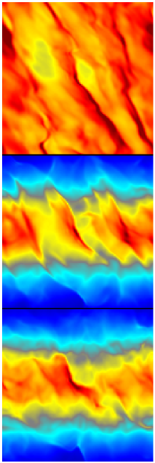
Figure 5: Colour image of density on slices through the fiducial model. The top panel shows an $x-y$ slice at $z=0$, the middle panel shows an $x-z$ slice at $y=0$, and the bottom panel shows a $y-z$ slice at $x=0$. Black is highest density, while blue is lowest.

6.3 Parameter study

We have explored the effect of each of the main model parameters on the development of the parametric instability and its non-linear outcome. A full list of relevant models, with model parameters, is given in Table 1. Run 1 is the fiducial model.

Table 1: List of all numerical models

No.	$L_{x}$	$L_{y}$	$L_{z}$	$n_{x}$	$n_{y}$	$n_{z}$	$S$
1	4	16	6	128	128	192	1	fiducial run
2	4	-	6	256	-	256	0.5
3	4	-	8	340	-	340	0.5
4	4	16	4	64	64	64	1
5	4	16	10	64	64	160	1
6	4	-	10	64	-	128	0.5	periodic, axisymm.
7	4	-	10	128	-	256	0.5	periodic, axisymm.
8	4	-	10	256	-	512	0.5	periodic, axisymm.
9	4	-	12	64	-	128	0.5	periodic, axisymm.
10	4	-	12	128	-	256	0.5	periodic, axisymm.
11	4	-	12	256	-	512	0.5	periodic, axisymm.
12	4	8	6	64	32	96	1
13	4	16	6	64	64	96	1
14	4	32	6	64	128	96	1
15	4	64	6	64	128	96	1
16	4	16	6	128	64	96	1
17	4	16	6	32	64	96	1
18	4	16	6	64	128	96	1
19	4	16	6	64	32	96	1
20	4	16	6	64	32	192	1
21	4	16	6	64	32	48	1
22	4	-	6	256	-	256	1	axisymm.
23	4	-	6	512	-	512	1	axisymm.
24	4	-	6	256	-	256	0.05	axisymm.
25	4	-	6	512	-	512	0.1	axisymm.
26	4	-	8	256	-	256	0.2	axisymm.
27	4	-	6	512	-	512	0.5	axisymm.
28	4	-	6	256	-	256	2	axisymm.
29	4	-	6	256	-	256	8	axisymm.

6.3.1 Vertical box size

One concern in formulating a numerical model such as this is whether an artificial aspect of the boundary conditions controls the outcome. In this respect, the azimuthal and radial boundary conditions are somewhat less worrisome than the vertical boundary conditions; the former restrict the scale of structure that can develop to the size of the box, while the latter introduces a reflection of outgoing waves that would otherwise dissipate in the disc atmosphere (although there could be a sharp boundary between a hot disc atmosphere and the body of the disc that would also produce reflections, albeit from a free rather than fixed boundary).

We have tested for variation in linear growth rate with the vertical size of box: compare, e.g., runs 2 and 3. Both runs give ${\rm d}\ln E_{{\rm k},z}/{\rm d}t\approx 0.25\Omega$. Thus for values of $L_{z}$ close to the fiducial value, $6H$, we observe no change in the numerically measured growth rate. For the non-linear development, we observe a trend in that the decay of epicyclic energy is slower in the larger boxes. Quantitatively, approximately $20\%$ more of the initial epicyclic energy is left in run 5 at $t=75\Omega^{-1}$ than in run 4 at the same instant. The small size of this effect suggests that the boundary condition is not controlling the outcome.

6.3.2 Type of vertical boundary condition

To test the effect of varying the character of the vertical boundary conditions, we performed a series of axisymmetric runs with periodic vertical boundary conditions (runs 6 to 11). These runs are special in that the initial conditions have

$$v_{x}=S(L_{z}/2\pi)\sin(2\pi z/L_{z})+\delta$$ (65)

to make them compatible with the boundary conditions. This velocity profile then requires $L_{z}$ larger than reflecting boundary condition runs so as to better approximate a linear shear near the mid-plane of the disc; this in turn implies lower numerical resolution $n_{z}/L_{z}$ for a given grid size $n_{z}$.

The growth rates measured in the periodic vertical runs are not distinguishably different from those measured in reflecting boundary condition runs at similar resolution. The decay of epicyclic energy also follows a similar trajectory under the two different boundary conditions. This again suggests that the boundary conditions are not controlling the outcome.

6.3.3 Azimuthal box size

One might be concerned that the limited azimuthal size of the box is somehow limiting the linear development of the instability or the non-linear outcome. This concern turns out to be justified over a limited range in $L_{y}$ for both the linear and non-linear development of the instability.

Figure 4 shows the evolution of ${\rm\,NA}_{1,2,3}$ in the fiducial run 1. This demonstrates that $m=1$ structure grows most quickly, and suggests that the low-$m$ modes available in a larger box might grow even more quickly. Figure 6 demonstrates that this is indeed the case. It shows the evolution of ${\rm\,NA}_{1}/L_{y}$ in runs 12, 13, 14, and 15, which have $L_{y}=8,16,32,64$ respectively. The numerical resolution $n_{y}/L_{y}$ is constant between these runs. The early growth of ${\rm\,NA}_{1}$ is strongest for $L_{y}=64$. In fact, the growth rate of ${\rm\,NA}_{1}$ for $L_{y}=64$ is $0.32\Omega$, close to the $0.42\Omega$ measured for ${\rm d}\ln E_{{\rm k},z}/{\rm d}t$. This evidence suggests that there is a non-axisymmetric counterpart of the parametric instability for, and only for, sufficiently low $m/L_{y}$.

Figure 6: Evolution of ${\rm\,NA}_{1}/L_{y}$ in runs with $L_{y}=8,16,32,$ and $64$. The ordinate units are arbitrary.

In retrospect this result is easy to understand. Our linear analysis could be trivially generalized to weakly non-axisymmetric disturbances using the shearing wave formalism of non-axisymmetric density wave theory (Goldreich & Lynden-Bell 1965). The radial wavenumber of the disturbance would then evolve according to $\dot{k}_{x}=q\Omega k_{y}$. The amplitudes of these shearing waves will grow so long as the radial wavenumber does not change so much over a growth time that the resonance between the daughter modes and parent mode is detuned.

The non-linear development of the instability is not strongly altered by variation of $L_{y}$. There is a tendency for $E_{\rm epi}$ to decay slightly more slowly in models with larger $L_{y}$. Presumably this is because large-scale, slowly dissipating motions are available in the large $L_{y}$ box, and these motions act as a reservoir for the epicyclic energy.

6.3.4 Numerical resolution

Runs 16 through 21, 1, 22, and 23 test the effect of numerical resolution. The measured linear growth rate is slightly dependent on resolution in the meridional plane. For $n_{x},n_{z}=32,48$, $\gamma_{\rm num}\equiv{\rm d}\ln E_{{\rm k},z}/{\rm d}t=0.37\Omega$; for $n_{x},n_{z}=64,96$, $\gamma_{\rm num}=0.46\Omega$; for $n_{x},n_{z}=128,192$, $\gamma_{\rm num}=0.49\Omega$; for $n_{x},n_{z}=512,512$, $\gamma_{\rm num}=0.53\Omega$. This should be compared to the linear theory rate $\gamma=0.65\Omega$. The non-linear decay rate of the warp also has a trend with resolution in that high resolution models decay more slowly.

6.3.5 Initial warp amplitude

At small $S/\Omega$, the three-mode coupling analysis of §5 predicts that

$${{\rm d}\ln E_{{\rm k},z}\over{{\rm d}t}}={3\sqrt{3}S\over{8}}\approx 0.65S.$$ (66)

To test this, we measured a numerical growth rate for a series of values of $S$. In each case, we used the run with the highest available numerical resolution in the meridional plane (we will be concerned only with the development of axisymmetric instabilities here). The results are listed in Table 2. The numerical growth rates typically lie $\approx 15\%$ below the analytic rates. We believe that this is primarily a resolution effect, since the growth rate grows monotonically with increasing resolution.

At large $S/\Omega$ the three-mode coupling analysis is no longer applicable. The incompressible, unstratified model of §4 is not limited to small $S/\Omega$, and numerical integrations of those model equations show reduced growth for $S/\Omega\mathrel{\hbox to0.0pt{\lower 3.0pt\hbox{$\mathchar 536\relax$}\hss}\raise 2.0pt\hbox{$\mathchar 318\relax$}}1$. This is observed in the numerical models listed in Table 2.

Table 2: List of measured and predicted values for growth rate

No.	$S/\Omega$	$\gamma_{\rm num}/\Omega$	$\gamma_{\rm th}/\Omega=3\sqrt{3}S/8$	$\gamma_{\rm num}/\gamma_{\rm th}$
24	0.05	0.020	0.032	0.62
26	0.1	0.055	0.065	0.85
26	0.2	0.11	0.13	0.85
27	0.5	0.28	0.32	0.87
23	1.0	0.49	0.65	0.76
28	2.0	0.82	1.3	0.63
29	8.0	1.7	5.2	0.33

7 Discussion

We have shown that warps in unmagnetized, non-self-gravitating, inviscid Keplerian discs are subject to an instability that leads, in the non-linear regime, to damping of the warp. The damping is non-linear in that the growth rate of the instability is proportional to the amplitude of the warp. How might this process influence the development of warps in astrophysical discs?

A full answer to this question awaits an understanding of other damping mechanisms that might act on a warp. If the disc is already turbulent, the parametric instability may not occur. In the Appendix, we estimate the influence of an isotropic effective turbulent viscosity on our analysis. We find that the instability still occurs if the amplitude of the in-plane oscillations is sufficiently large, possibly $S/\Omega\ga 30\alpha$, where $\alpha$ is the dimensionless viscosity parameter. In addition, for a given warping of the disc, $S/\Omega$ is reduced in the presence of viscosity because the resonance that drives the in-plane oscillations is weakened. Therefore our analysis is most relevant to discs with $\alpha\ll 1$.

Assuming that the instability develops into the non-linear regime, we may hazard a guess at the consequences for the warp, using a simple model for the interaction of in-plane and out-of-plane motions in the warp. We then apply the result to the warped, masing disc in NGC 4258.

Consider a linear, axisymmetric bending wave in the corotating frame. The radial and vertical displacements associated with the wave, $\xi_{r}\sim z\exp({\rm i}kr)$ and $\xi_{z}\sim\exp({\rm i}kr)$, obey

$${{\rm d}^{2}\xi_{r}\over{{\rm d}t^{2}}}+\kappa^{2}\xi_{r}=-{\rm i}k\xi_{z}\Omega^{2}z,$$ (67)

$${{\rm d}^{2}\xi_{z}\over{{\rm d}t^{2}}}+\Omega^{2}\xi_{z}={\rm i}kc_{\rm s}^{2}\xi_{r}{\partial}_{z}\xi_{r}.$$ (68)

It is evident that the in-plane and out-of-plane motions behave as coupled harmonic oscillators. If $k\sim r^{-1}$ and $H/r\ll 1$, as we shall assume, then the coupling is weak in the sense that $kc_{\rm s}\ll\Omega$. The coupling would be negligible except that $\kappa^{2}\simeq\Omega^{2}$ for a Keplerian disc, so the vertical and radial oscillations are resonant.

We will use equations (67,68) as the basis of a simple model for the warp. In addition to the terms from linear theory, we will include an out-of-plane driving term, meant to model the Pringle instability, and a non-linear damping term, meant to model the effects of the parametric instability. In terms of the normalized displacements $X_{z}=\xi_{z}/H$ and $X_{r}={\rm i}\xi_{r}(z=H)/H$, the governing equations are

$${{\rm d}^{2}X_{z}\over{{\rm d}t^{2}}}+\Omega^{2}X_{z}=-{\epsilon}\,\Omega^{2}X_{r}+\gamma\Omega{{\rm d}X_{z}\over{{\rm d}t}},$$ (69)

$${{\rm d}^{2}X_{r}\over{{\rm d}t^{2}}}+\kappa^{2}X_{r}=-{\epsilon}\,\Omega^{2}X_{z}-f(\dot{X}_{r}).$$ (70)

Here ${\epsilon}\equiv kc_{\rm s}/\Omega$, $\gamma/2$ is a dimensionless growth rate for the driving instability, and $f$ is some function of $\dot{X}_{r}\equiv{\rm d}X_{r}/{\rm d}t$ that models the damping effect of the parametric instability on in-plane motions.

We set $\kappa=\Omega=1$ and look for steady-state oscillatory solutions of equations (69, 70). To start, define “action-angle” variables by

$$X_{z} \equiv a_{z}\cos\theta_{z},~{}~{}~{}~{}\dot{X}_{z}\equiv-a_{z}\sin\theta_{z},$$ (71)

$$X_{r} \equiv a_{r}\cos\theta_{r},~{}~{}~{}~{}\dot{X}_{r}\equiv-a_{r}\sin\theta_{r}.$$ (72)

Consistency of these definitions requires

$$\dot{a}_{z}\cos\theta_{z}-\dot{\theta}_{z}a_{z}\sin\theta_{z} = -a_{z}\sin\theta_{z},$$ (73)

$$\dot{a}_{r}\cos\theta_{r}-\dot{\theta}_{r}a_{r}\sin\theta_{r} = -a_{r}\sin\theta_{r}.$$ (74)

These relations and the differential equations for $X_{r}$ and $X_{z}$ yield

$$\dot{a}_{z} = \gamma a_{z}\sin^{2}\theta_{z}+{\epsilon}a_{r}\cos\theta_{r}\sin\theta_{z},$$ (75)

$$\dot{a}_{r} = f\sin\theta_{r}+{\epsilon}a_{z}\sin\theta_{r}\cos\theta_{z},$$ (76)

$$\dot{\theta}_{z} = 1+\gamma\sin\theta_{z}\cos\theta_{z}+{\epsilon a_{r}\over a_{z}}\cos\theta_{r}\cos\theta_{z},$$ (77)

$$\dot{\theta}_{r} = 1+\frac{f}{a_{r}}\cos\theta_{r}+{\epsilon a_{z}\over a_{r}}\cos\theta_{r}\cos\theta_{z}.$$ (78)

When $\gamma$, ${\epsilon}$, and $f$ are $\ll 1$, the rapidly-oscillating terms can be averaged out:

$$\Delta\dot{\theta} \approx {{\epsilon}\over{2}}\left({a_{z}\over a_{r}}-{a_{r}\over a_{z}}\right)\cos\Delta\theta,$$ (79)

$$\dot{a}_{z} \approx {\gamma\over 2}a_{z}-{\epsilon\over 2}a_{r}\sin\Delta\theta,$$ (80)

$$\dot{a}_{r} \approx \bar{f}(a_{r})+{\epsilon\over 2}a_{z}\sin\Delta\theta,$$ (81)

where $\Delta\theta\equiv\theta_{r}-\theta_{z}$, $\bar{f}\equiv{\langle}f\sin\theta_{r}{\rangle}$, and ${\langle}{\rangle}$ denotes a phase average. Since $f$ should be an odd function of $\dot{X}_{r}$, we have $\langle f\cos\theta_{r}\rangle=0$.

A steady state requires either $a_{z}=a_{r}$ or $\cos\Delta\theta=0$. In astrophysical applications the latter solutions are likely to be more relevant, because thin discs with observable warps have $a_{z}\gg 1$, while $a_{r}\gg 1$ would require implausibly supersonic motions within the disc.

The steady state solutions with $\cos\Delta\theta=0$ have

$${\bar{f}(a_{r})\over{a_{r}}} = -{{\epsilon}^{2}\over{2\gamma}},$$ (82)

$$a_{z} = ({\epsilon}/\gamma)a_{r}.$$ (83)

Stability of this solution requires

$$a_{r}<a_{z}$$ (84)

and, for $n\equiv{\rm d}\ln\bar{f}/{\rm d}\ln a_{r}$,

$${\gamma^{2}\over{{\epsilon}^{2}}}<n<1.$$ (85)

To go further, we must guess at $\bar{f}(a_{r})$. At very small $a_{r}$, we expect $n\geq 2$ because the growth rate of the parametric instability is proportional to $a_{r}$. At larger amplitudes $f$ models the effect of stationary, fully developed turbulence. If turbulence initiated by the parametric instability acts as a viscosity (as might also be expected in an MHD turbulent disc) then $n\approx 1$. Notice that $n\approx 1$ is consistent with the approximately exponential damping of the warp observed in the numerical experiments of §6. The decay time of the epicyclic energy shown in Figure 2 is $\approx 30\Omega^{-1}$, which could be fitted by $f\approx a_{r}/60$: i.e., by a dimensionless viscosity $\alpha\approx 1.7\times 10^{-2}$.

Let us apply these results to the masing disc in NGC 4258 (Miyoshi et al. 1995, also Gammie et al. 1999 and references therein). The presence of water vapour suggests $c_{\rm s}\sim 1{\rm\,km\,sec^{-1}}$. The rotational velocity is $v_{c}\approx 1100(r/0.13{\rm\,pc})^{-1/2}{\rm\,km\,sec^{-1}}$. Thus ${\epsilon}\sim H/r\approx 10^{-3}$. The orientation of the inner edge of the masing disc at $\approx 0.13{\rm\,pc}$ differs from that at the outer edge at $\approx 0.24{\rm\,pc}$ by $\approx 0.25$ radians, so $a_{z}\approx 250$. The corresponding velocity of in-plane motions at $z=H$ would be $\approx 250{\rm\,km\,sec^{-1}}$, were linear theory applicable. Finally, an estimate of the growth time of the Pringle instability gives $\tau\sim 5\times 10^{6}{\rm\,yr}$ [Maloney et al. 1996], or $\gamma\equiv 2/(\Omega\tau)\sim 1.2\times 10^{-4}$ if $\Omega$ is taken at the outer edge of the disc. Direct measurements of maser velocities show that the departure from a Keplerian rotation curve is small, so we may take $\kappa=\Omega$.

Of the model parameters ${\epsilon},a_{z},$ and $\gamma$, the last is most uncertain. Let us assume that the disc is described by our model equations and is in equilibrium, then solve for $\gamma$. Suppose $f\approx\alpha\,{\rm sign}(\dot{X_{r}})|\dot{X_{r}}|^{n}/X_{0}^{n-1}$, where $X_{0}$ is a characteristic amplitude, and $n$ is just slightly smaller than $1$ so the equilibrium is stable. Here $\alpha$ is the dimensionless strength of the damping. For $n=1$ the damping rate is precisely what one would expect for a viscous disc with $\nu=\alpha c_{\rm s}^{2}/\Omega$. Then $\bar{f}=-\alpha p_{n+1}{\rm sign}(a_{r})|a_{r}|^{n}/X_{0}^{n-1}$, where $p_{n+1}\equiv\langle|\sin\theta_{r}|^{n+1}\rangle$, and

$$\gamma=(2\alpha p_{n+1})^{-1/n}{\epsilon}^{1+1/n}|a_{z}|^{-1+1/n}X_{0}^{1-1/n}.$$ (86)

In the limit $n\rightarrow 1$, $\gamma\rightarrow{\epsilon}^{2}/\alpha=10^{-6}/\alpha$. This is smaller than the nominal value by a factor of $100\alpha$.

We can obtain an upper limit on $\gamma$ if we suppose that the warp is limited by coupling to in-plane motions and that $a_{r}<1$. Then, to satisfy equation (83), we must have $\gamma<{\epsilon}/a_{z}\approx 4\times 10^{-6}$. This limit is due to the weakness of coupling between in-plane and out-of-plane motions. For larger growth rates the warp must be limited by some other process, or perhaps it is not limited and the disc is destroyed. The maximum dissipation rate to be expected of any local mechanism (one that relies upon the internal dynamics of the disc) is $\sim c_{\rm s}^{2}\Omega$ per unit mass. The local energy in vertical motions of the warp as measured in the corotating frame of the gas is $E_{\rm w}\sim\Omega^{2}\langle\xi_{z}^{2}\rangle$ per unit mass, and the rate at which the Pringle instability adds to this energy is

$$\gamma\Omega E_{\rm w}\sim 6\left(\frac{\gamma}{10^{-4}}\right)\left\langle\left(\frac{\xi_{z}}{250H}\right)^{2}\right\rangle~{}c_{\rm s}^{2}\Omega.$$

It is therefore difficult to see how any local mechanism can limit the warp if the growth rate is as large as Maloney et al.’s estimate.

Part of this discrepancy might be explained by uncertainties in the parameters of Maloney et al.’s model. It is also possible that non-linear effects reduce the growth rate of the Pringle instability. There is some evidence for this in that the disc in NGC 4258 is not as strongly twisted as one would expect from linear theory (see Herrnstein, 1997 for a warp model that fits the observations). Finally, non-linear effects may also enhance the coupling ${\epsilon}$ between in-plane and out-of-plane oscillations.

JG and CFG are supported by NASA Origins grant NAG5-8385. GIO is supported by Clare College, Cambridge. We thank the Isaac Newton Institute for their support during the programme on Dynamics of Astrophysical Discs, where this work was initiated. We also thank John Papaloizou and Caroline Terquem for their comments.

Appendix A Effect of viscosity on the instability

Here we make a rough estimate of the influence of pre-existing turbulence on the development of the parametric instability. In the absence of a proper understanding of the interaction of the in-plane oscillations with turbulence (see Torkelsson et al. 2000 for a direct numerical approach) we suppose that the process may be treated as an isotropic effective viscosity of the form

$$\nu=\alpha c_{\rm s}^{2}/\Omega=\alpha\Omega H^{2},$$ (87)

where $\alpha$ is the usual dimensionless viscosity parameter.

The Floquet analysis of §4 is easily adapted to include viscosity. The solution is identical but multiplied by the damping factor

$$\exp\left(-\int\nu k^{2}\,{\rm d}t\right).$$ (88)

When $S/\Omega$ is small the time-dependence of $k$ may be neglected and the growth rate of the instability is simply reduced according to

$$s\mapsto s-\nu k^{2}.$$ (89)

For a tuned mode with $k_{x}/k_{z}=\pm\sqrt{3}$, the modified growth rate is

$$s\approx{{3\sqrt{3}}\over{16}}S-4(k_{z}H)^{2}\alpha\Omega.$$ (90)

In the unstratified model $k_{z}$ is unrestricted, but, in reality, the mode must fit inside the disc. An approximate criterion can be obtained by requiring that at least half a wavelength fit into a vertical distance $2H$, i.e. $k_{z}H\ga\pi/2$. The instability then develops provided that

$${{S}\over{\Omega}}\ga 30\alpha.$$ (91)

The effect of a small viscosity on the mode-coupling analysis of §5 can also be estimated. Provided that bulk viscosity effects may be neglected, the eigenfunctions of wave modes in an isothermal disc (§3) can still be obtained in terms of Hermite polynomials when viscosity is included. The dispersion relation is much more complicated, but can be expanded for small $\alpha$ to obtain

$$\omega_{n}(k)=\omega_{n}^{(0)}(k)-{\rm i}\alpha\Omega d_{n}(k)+O(\alpha^{2}),$$ (92)

where the first term is the frequency in the inviscid case (equation 9) and $d_{n}$ is a dimensionless measure of the viscous damping rate of the mode. Generally speaking, $d_{n}$ increases with increasing $n$ and $k$. We therefore consider the first parametric resonance, which occurs between modes 1 and 2 (i.e. $\omega_{1}+\omega_{2}=\Omega$) at $kH\approx 1.88$. The inviscid growth rate is then $s\approx 0.138S$. At this point $d_{1}\approx d_{2}\approx 4.5$, giving a net growth rate of $0.138S-4.5\alpha\Omega$. The instability proceeds only if $S/\Omega\ga 33\alpha$, which agrees closely with equation (91).

References

- [Abramowitz & Stegun 1965] Abramowitz M., Stegun I. A., 1965, Handbook of Mathematical Functions, Dover, New York
- [Balbus & Hawley 1998] Balbus S. A., Hawley J. F., 1998, Rev. Mod. Phys., 70, 1
- [Bayly 1986] Bayly B. J., 1986, Phys. Rev. Lett., 57, 2160
- [Bender & Orszag 1978] Bender C. M., Orszag, S. A. 1978, Advanced Mathematical Methods for Scientists and Engineers, McGraw-Hill, New York
- [Craik & Criminale 1986] Craik A. D. D., Criminale W. O., 1986, Proc. R. Soc. Lond. A, 406, 13
- [Gammie 1996] Gammie C. F., 1996, ApJ, 457, 355
- [Gammie & Menou 1998] Gammie C. F., Menou K., 1998, ApJ, 492, 75
- [Gammie et al.1999] Gammie C. F., Narayan, R., & Blandford, R. 1999, ApJ, 516, 177
- [Goldreich & Lynden-Bell 1965] Goldreich P., Lynden-Bell D., 1965, MNRAS, 130, 125
- [Goodman 1993] Goodman J., 1993, ApJ, 406, 596
- [Hawley, Gammie & Balbus 1995] Hawley J. F., Gammie C. F., Balbus S. A., 1995, ApJ, 440, 742
- [Herrnstein 1997] Herrnstein, J. 1997, Ph.D. Thesis, Harvard University
- [Katz 1973] Katz J. I., 1973, Nat, 246, 87
- [Kelvin 1887] Lord Kelvin, 1887, Phil. Mag., 24, 188
- [Kumar & Goodman 1996] Kumar P., Goodman J., 1996, ApJ, 466, 946
- [Kumar & Coleman 1993] Kumar S., Coleman C. S., 1993, MNRAS, 260, 323
- [Lubow & Pringle 1993] Lubow S. H., Pringle J. E., 1993, ApJ, 409, 360
- [Maloney et al. 1996] Maloney, P., Begelman, M., & Pringle, J. 1996, ApJ, 472, 582
- [Maoz 1995] Maoz, E. 1995, ApJ, 447, L91
- [Miyoshi et al. 1995] Miyoshi M., Moran J., Herrnstein J., Greenhill L., Nakai N., Diamond P., Inoue M., 1995, Nat, 373, 127
- [Ogilvie 1999] Ogilvie G. I., 1999, MNRAS, 304, 557
- [Ogilvie & Lubow 1999] Ogilvie G. I., Lubow S. H., 1999, ApJ, 515, 767
- [Papaloizou & Lin 1995] Papaloizou J. C. B., Lin D. N. C., 1995, ApJ, 438, 841
- [Papaloizou & Terquem 1995] Papaloizou J. C. B., Terquem C., 1995, MNRAS, 274, 987
- [Pringle 1996] Pringle J. E., 1996, MNRAS, 281, 357
- [Roberts 1974] Roberts W. J., 1974, ApJ, 187, 575
- [Sagdeev & Galeev 1969] Sagdeev R. Z., Galeev A. A., 1969, Nonlinear plasma theory, Benjamin, New York
- [Stone & Norman 1992] Stone J. M., Norman M. L., 1992, ApJS, 80, 753
- [Tananbaum et al. 1972] Tananbaum H., Gursky H., Kellogg E. M., Levinson R., Schreier E., Giacconi R., 1972, ApJ, 174, L143
- [Torkelsson et al. 2000] Torkelsson U., Ogilvie G. I., Brandenburg A., Pringle J. E., Nordlund Å, Stein R. F., 2000, MNRAS, in press