THE EQUATION OF STATE OF NEUTRON-STAR MATTER IN STRONG MAGNETIC FIELDS

Abstract

We study the effects of very strong magnetic fields on the equation of state (EOS) in multicomponent, interacting matter by developing a covariant description for the inclusion of the anomalous magnetic moments of nucleons. For the description of neutron star matter, we employ a field-theoretical approach which permits the study of several models which differ in their behavior at high density. Effects of Landau quantization in ultra-strong magnetic fields ($B>10^{14}$ Gauss) lead to a reduction in the electron chemical potential and a substantial increase in the proton fraction. We find the generic result for $B>10^{18}$ Gauss that the softening of the EOS caused by Landau quantization is overwhelmed by stiffening due to the incorporation of the anomalous magnetic moments of the nucleons. In addition, the neutrons become completely spin polarized. The inclusion of ultra-strong magnetic fields leads to a dramatic increase in the proton fraction, with consequences for the direct Urca process and neutron star cooling. The magnetization of the matter never appears to become very large, as the value of $|H/B|$ never deviates from unity by more than a few percent. Our findings have implications for the structure of neutron stars in the presence of large frozen-in magnetic fields.

Subject headings: stars: neutron stars – equation of state – stars: magnetic fields

1 INTRODUCTION

Recent observational and theoretical studies motivate the investigation of the effects of ultra-strong magnetic fields ($B>10^{14}$ Gauss) on neutron stars. Several independent arguments link the class of soft $\gamma-$ray repeaters and perhaps certain anomalous X-ray pulsars with neutron stars having ultra strong magnetic fields – the so-called magnetars (Paczyński 1992; Thompson & Duncan 1995, 1996; Melatos 1999). In addition, two of the four known soft $\gamma-$ray repeaters directly imply, from their periods and spin-down rates, surface fields in the range $2-8\times 10^{14}$ Gauss. Kouveliotou et al. (1998, 1999) argue from the population statistics of soft $\gamma-$ray repeaters that magnetars constitute about 10% of the neutron star population. While some observed white dwarfs have large enough fields to give ultra-strong neutron star magnetic fields through flux conservaton, it does not appear likely that such isolated examples could account for a significant fraction of ultra-strong field neutron stars. Therefore, an alternative mechanism seems necessary for the creation ultra-strong magnetic fields in neutron stars. Duncan & Thompson (1992, 1996) suggested that large fields (up to $3\times 10^{17}\times(1\rm{~{}ms}/P_{i})$ Gauss, where $P_{i}$ is the initial rotation period) can be generated in nascent neutron stars through the smoothing of differential rotation and convection.

These developments raise the intriguing questions:
(1) What is the largest frozen-in magnetic field a stationary neutron star can sustain?, and,
(2) What is the effect of such ultra-strong magnetic fields on the maximum neutron star mass?

The answers to both of these questions hinge upon the effects strong magnetic fields have both on the equation of state (EOS) of neutron-star matter and on the structure of neutron stars. In this paper, we will focus on the effects of strong magnetic fields on the EOS. Subsequent work will be devoted to investigating the effects of strong fields on the structure of neutron stars, incorporating the EOSs developed in this work.

The magnitude of the magnetic field strength $B$ needed to dramatically affect neutron star structure directly can be estimated with a dimensional analysis (Lai & Shapiro 1991) equating the magnetic field energy $E_{b}\sim(4\pi R^{3}/3)(B^{2}/8\pi)$ with the gravitational binding energy $E_{B.E.}\sim GM^{2}/R$, yielding $B\sim 2\times 10^{18}\left(M/1.4{\rm M}_{\odot}\right)\left(R/10\ {\rm km}\right)^{-2}$ Gauss, where $M$ and $R$ are, respectively, the neutron star mass and radius.

The magnitude of $B$ required to directly influence the EOS can be estimated by considering its effects on charged particles. Charge neutral, beta-equilibrated, neutron-star matter contains both negatively charged leptons (electrons and muons) and positively charged protons. Magnetic fields quantize the orbital motion (Landau quantization) of these charged particles. Relativistic effects become important when the particle’s cyclotron energy $e\hbar~{}B/(mc)$ is comparable to it’s mass (times $c^{2}$). The magnitudes of the so-called critical fields are $B_{c}^{e}=(\hbar c/e)\mathrel{\hbox to0.0pt{ \raise 3.0pt\hbox{\hskip-1.75pt-}\hss}\hbox{$\lambda_{e}$}}^{-2}=4.414\times 10^{13}$ Gauss and $B_{c}^{p}=(m_{p}/m_{e})^{2}B_{c}^{e}=1.487\times 10^{20}$ Gauss for the electron and proton, respectively ( $\mathrel{\hbox to0.0pt{ \raise 3.0pt\hbox{\hskip-1.75pt-}\hss}\hbox{$\lambda_{e}$}}=\hbar/m_{e}c\simeq 386$ fm is the Compton wavelength of the electron). It will be convenient to measure the field strength $B$ in units of $B_{e}^{c}$, viz., $B^{*}\equiv B/B^{c}_{e}$. When the Fermi energy of the proton becomes significantly affected by the magnetic field, the composition of matter in beta equilibrum is significantly affected. In turn, the pressure of matter is significantly affected. We show that this occurs when $B^{*}\sim 10^{5}$, and will lead to a general softening of the EOS.

In neutron stars, magnetic fields may well vary in strength from the core to the surface. The scale lengths of such variations are, however, usually much larger than the microscopic magnetic scale $l_{m}$, which depends on the magnitude of $B$. For low fields, for which the quasi-classical approximation holds, $l_{m}\simeq(\mathrel{\hbox to0.0pt{ \raise 3.0pt\hbox{\hskip-1.75pt-}\hss}\hbox{$\lambda_{e}$}}^{2}/B^{*})(3\pi^{2}n_{e})^{1/3}\approx 10^{5}(n_{e}/n_{s})^{1/3}/B^{*}$ fm, where $n_{e}$ is the number density of electrons and $n_{s}$ is the normal nuclear saturation density (about 0.16 fm^-3). For high fields, when only a few Landau levels are occupied, $l_{m}\simeq 2\pi^{2}n_{e}(\mathrel{\hbox to0.0pt{ \raise 3.0pt\hbox{\hskip-1.75pt-}\hss}\hbox{$\lambda_{e}$}}^{2}/B^{*})^{2}\approx 7\times 10^{9}(n_{e}/n_{s})/B^{*2}$ fm. In either case, the requirement that $R>>l_{m}$ is amply satisfied; hence, the magnetic field $B$ may be assumed to be locally constant and uniform as far as effects on the EOS are concerned.

In non-magnetic neutron stars, the pressure of matter ranges from $2-5~{}{\rm MeV~{}fm}^{-3}$ at nuclear density to $200-600~{}{\rm MeV~{}fm}^{-3}$ at the central density of the maximum mass configuration, depending on the EOS (Prakash et al. 1997). These values may be contrasted with the energy density and pressure from the electromagnetic field: $\varepsilon_{f}=P_{f}=B^{2}/(8\pi)=4.814\times 10^{-8}B^{*~{}2}~{}{\rm MeV~{}fm}^{-3}$. The field contributions can dominate the matter pressure for $B^{*}>10^{4}$ at nuclear densities and for $B^{*}>10^{5}$ at the central densities of neutron stars, and must therefore be included whenever the field dramatically influences the star’s composition and matter pressure.

In strong magnetic fields, contributions from the anomalous magnetic moments of the nucleons must also be considered. Experimentally, $\kappa_{p}=\mu_{N}\left(g_{p}/2-1\right)$ for the proton, $\kappa_{n}=\mu_{N}g_{n}/2$ for the neutron, where $\mu_{N}$ is the nuclear magneton and $g_{p}=5.58$ and $g_{n}=-3.82$ are the Landé g-factors for the proton and neutron, respectively. The energy $|\kappa_{n}+\kappa_{p}|B\simeq 1.67\times 10^{-5}B^{*}$ MeV measures the changes in the beta equilibrium condition and to the baryon Fermi energies. Since the Fermi energies range from a few MeV to tens of MeV for the densities of interest, it is clear that contributions from the anomalous magnetic moments also become significant for $B^{*}>10^{5}$. We demonstrate that for such fields, complete spin polarization of the neutrons occurs, which results in an overall stiffening of the EOS that overwhelms the softening induced by Landau quantization.

In magnetized matter, the stress energy tensor contains terms proportional to $HB$, where $H=B+4\pi{\cal M}$ and ${\cal M}$ is the magnetization (Landau, Lifshitz & Pitaevskiĭ 1984). Thus, extra terms, in addition to the usual ones proportional to $B^{2}$, are introduced into the structure equations (Cardall et al. 1999). The magnetization in a single component electron gas has been studied extensively (Blandford & Hernquist 1982) for neutron star crust matter. We generalize this formulation to the case of interacting multicomponent matter with and without the effects of the anomalous magnetic moments. We find that deviations of $H$ from $B$ occur for field strengths $B^{*}\gtrsim 10^{5}$.

Although the effects of magnetic fields on the EOS at low densities, relevant for neutron star crusts, has been extensively studied (see for example, Canuto & Ventura 1977; Fushiki, Gudmundsson & Pethick 1989; Fushiki et al. 1992; Abrahams & Shapiro 1991; Lai & Shapiro 1991; Rögnvaldsson et al. 1993, Thorlofsson et al. 1998), only a handful of previous works have considered the effects of very large magnetic fields on the EOS of dense neutron star matter (Chakrabarty 1996; Chakrabarty, Bandyopadhyay, & Pal 1997, Yuan & Zhang 1999). Lai and Shapiro (1991) considered non-interacting, charge neutral, beta-equilibrated matter at subsaturation densities, while Chakrabarty and co-authors studied dense matter including interactions using a field-theoretical description. These authors found large compositional changes in matter induced by ultra-strong magnetic fields due to the quantization of orbital motion. Acting in concert with the nuclear symmetry energy, Landau quantization substantially increases the concentration of protons compared to the field-free case, which in turn leads to a softening of the EOS. This lowers the maximum mass relative to the field-free value. In these works, however, the electromagnetic field energy density and pressure, which tend to stiffen the EOS, were not included. In addition, changes in the general relativistic structure induced by the magnetic fields (studied in detail by Bocquet et al. 1995 who, however, omitted the compositional changes in the EOS due to Landau quantization) were also ignored. Thus, the combined effects of the magnetic fields on the EOS and on the general relativistic structure remain to be determined.

Compared to these earlier works, we make several improvements in the calculation of the EOS. These improvements include (1) a study of a larger class of field-theoretical models in order to extract the generic trends induced by Landau quantization, (2) the development of a covariant description for the inclusion of the anomalous magnetic moments of the nucleons, and (3) a detailed study of magnetization of interacting multicomponent matter with and without the inclusion of the anomalous magnetic moments. We also provide simple analytical estimates of when each of these effects begin to significantly influence the EOS. Our future work will employ the EOSs developed in this work to complete a fully self-consistent calculation of neutron star structure including the combined effects of the direct effects of magnetic fields on the EOS and general relativistic structure.

In §2, we present the field-theoretical description of dense neutron star matter including the effects of Landau quantization and the nucleon anomalous magnetic moments. Section 3 contains a detailed study of the effects of Landau quantization on the EOS for two classes of Lagrangians. In addition to providing contrasts with earlier work, our results highlight the extent to which the underlying interactions affect the basic findings. This section also includes new theoretical developments concerning the magnetization of interacting, multicomponent matter. Section 4 is devoted to the effects of the anomalous magnetic moments on the EOS. Here results for a charge neutral neutron, proton, electron, and muon gas are compared with those for interacting matter to asses the generic trends. Our conclusions and outlook, including the possible effects of additional components such as hyperons, Bose condensates and quarks, are presented in §5. The covariant description for the inclusion of the anomalous magnetic moments of the nucleons is presented in the Appendix, where explicit formulae for the nucleon Dirac spinors and energy spectra are derived. Except where necessary, we use units wherin $\hbar$ and $c$ are set to unity.

2 THEORETICAL FRAMEWORK

For the description of the EOS of neutron-star matter, we employ a field-theoretical approach in which the baryons (neutrons, $n$, and protons, $p$) interact via the exchange of $\sigma~{}-\omega~{}-\rho$ mesons. We study two classes of models, which differ in their behavior at high density. The Lagrangian densities associated with these two classes are (Boguta & Bodmer 1977, Zimanyi & Moszkowski 1990)

$${\cal L}_{I} = {\cal L}_{b}-\left(1-\frac{g_{\sigma_{b}}\sigma}{m_{b}}\right)\overline{\Psi}_{b}m_{b}\Psi_{b}+{\cal L}_{m}+{\cal L}_{l}\,,$$

$${\cal L}_{II} = \left(1+\frac{g_{\sigma_{b}}\sigma}{m_{b}}\right){\cal L}_{b}-\overline{\Psi}_{b}m_{b}\Psi_{b}+{\cal L}_{m}+{\cal L}_{l}\,.$$ (1)

The baryon ($b=n,p$), lepton ($l=e,\mu$), and meson ($\sigma,~{}\omega,~{}{\rm and}~{}\rho$) Lagrangians are given by

$${\cal L}_{b} = \overline{\Psi}_{b}\left(i\gamma_{\mu}\partial^{\mu}+q_{b}\gamma_{\mu}A^{\mu}-g_{\omega_{b}}\gamma_{\mu}\omega^{\mu}-g_{\rho_{b}}\tau_{3_{b}}\gamma_{\mu}\rho^{\mu}-\kappa_{b}\sigma_{\mu\nu}F^{\mu\nu}\right)\Psi_{b}\,,$$

$${\cal L}_{l} = \overline{\psi}_{l}\left(i\gamma_{\mu}\partial^{\mu}+q_{l}\gamma_{\mu}A^{\mu}\right)\psi_{l}\,,$$

$${\cal L}_{m} = \frac{1}{2}\partial_{\mu}\sigma\partial^{\mu}\sigma-\frac{1}{2}m_{\sigma}^{2}\sigma^{2}-U(\sigma)+\frac{1}{2}m_{\omega}^{2}\omega_{\mu}\omega^{\mu}-\frac{1}{4}\Omega^{\mu\nu}\Omega_{\mu\nu}$$ (2)

$$\mbox{}+\frac{1}{2}m_{\rho}^{2}\rho_{\mu}\rho^{\mu}-\frac{1}{4}P^{\mu\nu}P_{\mu\nu}-\frac{1}{4}F^{\mu\nu}F_{\mu\nu}\,,$$

where $\Psi_{b}$ and $\psi_{l}$ are the baryon and lepton Dirac fields, respectively. The nucleon mass and the isospin projection are denoted by $m_{b}$ and $\tau_{3_{b}}$, respectively. The mesonic and electromagnetic field strength tensors are given by their usual expressions: $\Omega_{\mu\nu}=\partial_{\mu}\omega_{\nu}-\partial_{\nu}\omega_{\mu}$, $P_{\mu\nu}=\partial_{\mu}\rho_{\nu}-\partial_{\nu}\rho_{\mu}$, and $F_{\mu\nu}=\partial_{\mu}A_{\nu}-\partial_{\nu}A_{\mu}$. The strong interaction couplings are denoted by $g$, the electromagnetic couplings by $q$, and the meson masses by $m$ all with appropriate subscripts. The anomalous magnetic moments are introduced via the coupling of the baryons to the electromagnetic field tensor with $\sigma_{\mu\nu}=\frac{i}{2}\left[\gamma_{\mu},\gamma_{\nu}\right]$ and strength $\kappa_{b}$. We will contrast results for cases with $\kappa_{b}=0$ and $\kappa_{b}$ taken to be their measured values. The quantity $U(\sigma)$ denotes possible scalar self-interactions. It is straightforward to include self interactions between both the vector $\omega$ and the iso-vector $\rho$ mesons (Müller & Serot 1996). Although the electromagnetic field is included in ${\cal L}_{I}$ and ${\cal L}_{II}$, it assumed to be externally generated (and thus has no associated field equation) and only frozen-field configurations will be considered.

The thermodynamic quantities will be evaluated in the mean field approximation, in which the mesonic fields are assumed to be constant. The field equations are

$$m_{\sigma}^{2}\langle\sigma\rangle+\frac{\partial U(\sigma)}{\partial\sigma}=\left\{\begin{array}[]{cl}\sum_{b}g_{\sigma_{b}}n^{s}_{b}&\mbox{for ${\cal L}_{I}$}\\ \sum_{b}g_{\sigma_{b}}\left(\frac{m_{b}^{*}}{m_{b}}\right)^{2}n^{s}_{b}&\mbox{for ${\cal L}_{II}$ \,,}\end{array}\right.$$ (3)

$$m_{\omega}^{2}\langle\omega^{0}\rangle=\sum_{b}g_{\omega_{b}}n_{b}\,,$$ (4)

$$m_{\rho}^{2}\langle\rho^{0}\rangle=\sum_{b}g_{\rho_{b}}\tau_{3_{b}}n_{b}\,,$$ (5)

$$\left[\vec{\alpha}{{\scriptscriptstyle\stackrel{{\scriptstyle\bullet}}{{{}}}}}\left(\vec{p}-q_{l}\vec{A}\right)+\beta m_{l}\right]\psi_{l}=E\psi_{l}\,,$$ (6)

$$\left[\vec{\alpha}{{\scriptscriptstyle\stackrel{{\scriptstyle\bullet}}{{{}}}}}\left(\vec{p}-q_{b}\vec{A}\right)+\beta m_{b}^{*}\right]\Psi_{b}=(E-g_{\omega_{b}}\omega^{0}-g_{\rho_{b}}\tau_{3_{b}}\rho^{0})\Psi_{b}\,,$$ (7)

where the effective baryon masses are

$$\frac{m_{b}^{*}}{m_{b}}=\left\{\begin{array}[]{cl}\left(1-\frac{g_{\sigma_{b}}\sigma}{m_{b}}\right)&\mbox{for ${\cal L}_{I}$}\\ \left(1+\frac{g_{\sigma_{b}}\sigma}{m_{b}}\right)^{-1}&\mbox{for ${\cal L}_{II}$ \,,}\end{array}\right.$$ (8)

and $n_{b}^{s}$ is the scalar number density. The scalar self-interaction is taken to be of the form (Boguta & Bodmer 1977; Glendenning 1982, 1985)

$$U(\sigma)=\frac{1}{3}bm_{n}(g_{\sigma_{n}}\sigma)^{3}+\frac{1}{4}c(g_{\sigma_{n}}\sigma)^{4}\,,$$ (9)

where the $m_{n}$ in the first term is included to make $b$ dimensionless. In charge neutral, beta equilibrated matter, the conditions

$$\mu_{n}-\mu_{p}=\mu_{e}=\mu_{\mu}\,,$$ (10)

$$n_{p}=n_{e}+n_{\mu}\,,$$ (11)

also apply. Given the nucleon-meson coupling constants and the coefficients in the scalar self-interaction, equations (3) through (11) may be solved self consistently for the chemical potentials, $\mu_{i}$, and the field strengths, $\sigma$, $\omega^{0}$, and $\rho^{0}$.

3 EFFECTS OF LANDAU QUANTIZATION

From equation (6), the energy spectrum for the leptons is (see, for example, Canuto & Ventura 1977)

$$E_{l}=\sqrt{k_{z}^{2}+\widetilde{m}^{l~{}2}_{n,\sigma_{z}}}\,,$$ (12)

where

$$\widetilde{m}_{n,\sigma_{z}}^{l~{}2}=m_{l}^{2}+2\left(n+\frac{1}{2}-\frac{1}{2}\frac{q_{l}}{|q_{l}|}\sigma_{z}\right)|q_{l}|B\,.$$ (13)

Here, $n$ is the principal quantum number and $\sigma_{z}$ (not to be confused with the scalar field $\sigma$) is the spin along the magnetic field axis. $k_{z}$ is the component of the momentum along the magnetic field axis. The quantity $\nu=n+1/2-(1/2)(q_{i}/|q_{i}|)\sigma_{z}$ characterizes the so-called Landau level. Equation (7) gives the energy spectrum for the protons as

$$E_{p}=\sqrt{k_{z}^{2}+\widetilde{m}^{p~{}2}_{n,\sigma_{z}}}+g_{\omega_{p}}\omega^{0}-g_{\rho_{p}}\frac{1}{2}\rho^{0}\,,$$ (14)

where $\widetilde{m}^{p}_{n,\sigma_{z}}$ is obtained by replacing $m_{l}$ on the right hand side of equation (13) by $m^{*}_{p}$. The neutron energy spectrum is that of the free Dirac particle, but with shifts arising from the scalar, vector, and isovector interactions:

$$E_{n}=\sqrt{k^{2}+m_{n}^{*~{}2}}+g_{\omega_{n}}\omega^{0}+g_{\rho_{n}}\frac{1}{2}\rho^{0}\,.$$ (15)

At zero temperature and in the presence of a constant magnetic field $B$, the number and energy densities of charged particles are given by

$$n_{i=l,p}=\frac{|q_{i}|B}{2\pi^{2}}\sum_{\sigma_{z}}\sum_{n=0}^{n_{max}}k_{f,n,\sigma_{z}}^{i}\,,$$ (16)

$$\varepsilon_{i=l,p}=\frac{|q_{i}|B}{4\pi^{2}}\sum_{\sigma_{z}}\sum_{n=0}^{n_{max}}\left[E_{f}^{i}k_{f,n,\sigma_{z}}^{i}+\widetilde{m}_{n,\sigma_{z}}^{i~{}2}\ln\left(\left|\frac{E_{f}^{i}+k_{f,n,\sigma_{z}}^{i}}{\widetilde{m}^{i}_{n,\sigma_{z}}}\right|\right)\right]\,.$$ (17)

Above, $k_{f,n,\sigma_{z}}^{i}$ is the Fermi momentum for the level with the principal quantum number $n$ and spin $\sigma_{z}$ and is given by

$$k_{f,n,\sigma_{z}}^{i~{}2}=E_{f}^{i~{}2}-\widetilde{m}_{n,\sigma_{z}}^{i~{}2}\,.$$ (18)

The summation in equation (16) is terminated at $n_{max}$, which is the integer preceeding the value of $n$ for which $k_{f,n,\sigma_{z}}^{i~{}2}$ is negative. The Fermi energies are fixed by the chemical potentials

$$E_{f}^{l}=\mu_{l}\,,$$ (19)

$$E_{f}^{b}=\mu_{b}-g_{\omega_{b}}\omega^{0}-g_{\rho_{b}}\tau_{3_{b}}\rho^{0}\,.$$ (20)

For the protons, the scalar number density may be determined to be (Chakrabarty 1996)

$$n_{p}^{s}=\frac{|q_{p}|Bm^{*}_{p}}{2\pi^{2}}\sum_{\sigma_{z}}\sum_{n=0}^{n_{max}}\ln\left(\left|\frac{E_{f}^{p}+k_{f,n,\sigma_{z}}^{p}}{\widetilde{m}_{n,\sigma_{z}}^{p}}\right|\right)\,.$$ (21)

The number, energy, and scalar number densities of the neutrons are unchanged in form from the field-free case

$$n_{n}=\frac{k_{f}^{n~{}3}}{3\pi^{2}}\,,$$ (22)

$$n^{s}_{n}=\frac{m_{n}^{*}}{2\pi^{2}}\left[E_{f}^{n}k_{f}^{n}-m_{n}^{*~{}2}\ln\left(\left|\frac{E_{f}^{n}+k_{f}^{n}}{m_{n}^{*}}\right|\right)\right]\,,$$ (23)

$$\varepsilon_{n}=\frac{1}{8\pi^{2}}\left[2E_{f}^{n~{}3}k_{f}^{n}-m_{n}^{*~{}2}E_{f}^{n}k_{f}^{n}-m_{n}^{*~{}4}\ln\left(\left|\frac{E_{f}^{n}+k_{f}^{n}}{m_{n}^{*}}\right|\right)\right]\,.$$ (24)

The total energy density of the system is

$$\varepsilon = \frac{1}{2}m_{\omega}^{2}\omega_{0}^{2}+\frac{1}{2}m_{\rho}^{2}\rho_{0}^{2}+\frac{1}{2}m_{\sigma}^{2}\sigma^{2}+U(\sigma)$$ (25)

$$\mbox{}+\sum_{b}\varepsilon_{b}+\sum_{l}\varepsilon_{l}+\frac{B^{2}}{8\pi^{2}}\,,$$

where the last term is the contribution from the electromagnetic field. Use of equations (10) and (11), which are satisfied in charge neutral beta-equilibrated matter, in the general expression for the pressure, $P=\sum_{i}\mu_{i}n_{i}-\varepsilon$ ($i=n,p,e,~{}{\rm and}~{}\mu$), allows the pressure to be written only in terms of the neutron chemical potential through the relation $P=\mu_{n}n_{b}-\varepsilon$. In fact, utilizing the appropriate relations satisfied by the various chemical potentials and the number densities involved in the charge neutrality condition, it is easily verified that this relation is satisfied even in the presence of additional components such as strangeness-bearing hyperons, Bose condensates (pion or kaon), and quarks, which may likely exist in dense neutron-star matter.

3.1 Magnetization

The magnetic field strength, $H$, is related to the energy density by (Landau, Lifshitz & Pitaevskiĭ 1984)

$$H=4\pi\left(\frac{\partial\varepsilon}{\partial B}\right)_{n_{b}}=B+4\pi{\cal M}\,,$$ (26)

where ${\cal M}$ is the magnetization. This is equivalent to the set of equations

$$\frac{dn_{b}}{dB} = 0\,,$$

$${\cal M} = \frac{\partial\varepsilon_{l}}{\partial B}+\frac{\partial\varepsilon_{l}}{\partial E_{f}^{l}}\frac{dE_{f}^{l}}{dB}+\frac{\partial\varepsilon_{p}}{\partial B}+\frac{\partial\varepsilon_{p}}{\partial E_{f}^{p}}\frac{dE_{f}^{p}}{dB}+\frac{\partial\varepsilon_{n}}{\partial B}+\frac{\partial\varepsilon_{n}}{\partial E_{f}^{n}}\frac{dE_{f}^{n}}{dB}$$ (27)

$$\mbox{}+m_{\rho}^{2}\rho^{0}\frac{d\rho^{0}}{dB}+m_{\omega}^{2}\omega^{0}\frac{d\omega^{0}}{dB}+\frac{\partial\varepsilon}{\partial\sigma}\frac{d\sigma}{dB}\,.$$

The first of these gives

$$\frac{\partial n_{n}}{\partial E_{f}^{n}}\frac{dE_{f}^{n}}{dB}=-\frac{\partial n_{n}}{\partial B}-\frac{\partial n_{p}}{\partial B}-\frac{\partial n_{p}}{\partial E_{f}^{p}}\frac{dE_{f}^{p}}{dB}\,.$$ (28)

Using the conditions of charge neutrality and chemical equilibrium, one has

$$\frac{\partial n_{l}}{\partial E_{f}^{l}}\frac{dE_{f}^{l}}{dB}=-\frac{\partial n_{l}}{\partial B}+\frac{\partial n_{p}}{\partial B}+\frac{\partial n_{p}}{\partial E_{f}^{p}}\frac{dE_{f}^{p}}{dB}\,.$$ (29)

From the field equations and the definition of the scalar density,

$$\frac{d\omega^{0}}{dB} = \frac{g_{\omega}}{m_{\omega}^{2}}\frac{dn_{b}}{dB}=0\,,$$

$$\frac{d\rho^{0}}{dB} = \frac{g_{\rho}}{m_{\rho}^{2}}\frac{1}{2}\frac{d}{dB}\left(n_{n}-n_{p}\right)=-\frac{g_{\rho}}{m_{\rho}^{2}}\frac{dn_{p}}{dB}\,,$$

$$\frac{\partial\varepsilon}{\partial\sigma} = 0\,.$$ (30)

Note also that

$$\frac{\partial\varepsilon_{i}}{\partial E_{f}^{i}}=E_{f}^{i}\frac{\partial n_{i}}{\partial E_{f}^{i}}\,.$$ (31)

Utilizing these results, equation (26) becomes

$${\cal M}=T_{I}+T_{II}\frac{\partial n_{p}}{\partial E_{f}^{p}}\frac{dE_{f}^{p}}{dB}\,,$$ (32)

where

$$T_{I} = \frac{\partial\varepsilon_{l}}{\partial B}-E_{f}^{l}\frac{\partial n_{l}}{\partial B}+\frac{\partial\varepsilon_{n}}{\partial B}-E_{f}^{n}\frac{\partial n_{n}}{\partial B}+\frac{\partial\varepsilon_{p}}{\partial B}$$

$$+\left(E_{f}^{l}-E_{f}^{n}-g_{\rho}\rho^{0}\right)\frac{\partial n_{p}}{\partial B}\,,$$

$$T_{II} = E_{f}^{l}+E_{f}^{p}-E_{f}^{n}-g_{\rho}\rho^{0}\,.$$ (33)

Note that chemical equilibrium ensures that $T_{II}=0$ whence the magnetization takes the general form

$${\cal M}=\sum_{i=e,\mu,p,n}\left(\frac{\partial\varepsilon_{i}}{\partial B}-E_{f}^{i}\frac{\partial n_{i}}{\partial B}\right)\,.$$ (34)

In the case under current consideration, inserting the explicit forms of the energy density and number density yields the result

$${\cal M}=\sum_{i=e,\mu,p}\left[\frac{\varepsilon_{i}-E_{f}^{i}n_{i}}{B}+\frac{B}{2\pi^{2}}\sum_{\sigma_{z}}\sum_{n=0}^{n_{max}}\left(n+\frac{1}{2}-\frac{1}{2}\sigma_{z}\right)\ln\left(\left|\frac{E_{f}^{i}+k_{f,n,\sigma_{z}}^{i}}{\widetilde{m}_{n,\sigma_{z}}^{i}}\right|\right)\right]\,.$$ (35)

This result generalizes the result of Blandford & Hernquist (1982) for an electron gas to the case of a multi-component system including interacting nucleons. That the functional form of ${\cal M}$ for interacting nucleons is the same as that for non-interacting particles stems from the fact that, in the mean field approximation, the field equations for the nucleons reduces to the Dirac equation for a free particle, but with an effective mass $m^{*}$.

3.2 Results

In Table 1, we list the various nucleon-meson and meson self-interaction couplings for the two classes of models chosen for this study. In each case, the couplings were chosen to reproduce commonly accepted values of the equilibrium nuclear matter properties: the binding energy per particle $B/A$, the saturation density $n_{s}$, the Dirac effective mass $m_{n}^{*}/m_{n}$, the compression modulus $K_{0}$, and the symmetry energy $a_{\mbox{\tiny sym}}$. The high-density behavior of the EOS is sensitive to the strength of the meson couplings employed and the models chosen encompass a fairly wide range of variation. The HS81 model, which has a rather high compression modulus, allows us to contrast our results with those of Chakrabarty (1996) who also used HS81 in the case when Landau quantization is considered, and to assess the effects of the inclusion of magnetic moments. Models HS81 and GM1–GM3 employ linear scalar couplings (${\cal L}_{I}$), while the ZM model employs a nonlinear scalar coupling (${\cal L}_{II}$), which is reflected in the high density behaviors of $m_{n}^{*}/m_{n}$. Thus, comparison of the HS81, GM1–GM3 and ZM models allows us to contrast the effects of the underlying EOS.

In Figure 1, we show results of some physical quantitites of interest for our baseline case, model GM3. At supernuclear densities and in the absence of a magnetic field, the matter pressure is dominated by the baryons principally due to the repulsive nature of the strong interactions. Even up to the central density in a neutron star, the proton fraction remains sufficiently small that the neutrons dominate the total pressure.

The magnitude of the magnetic field $B$ required to induce significant changes in the EOS may be estimated in a straightforward manner. In the presence of a magnetic field, the contributions from the protons become significant when only one Landau level is occupied, i.e., when the protons are completely spin polarized. This happens when $q_{p}B/\hbar c>(2\pi^{4}n_{p}^{2})^{1/3}$. Therefore, we arrive at the estimate $B^{*}>\mathrel{\hbox to0.0pt{ \raise 3.0pt\hbox{\hskip-1.75pt-}\hss}\hbox{$\lambda_{e}$}}^{2}(2\pi^{4}Y_{p}^{2}n_{b}^{2})^{1/3}$ for quantum effects to dominate. The proton fraction $Y_{p}=n_{p}/n_{b}$, which depends upon both the density and the magnetic field, typically lies in the range 0.1–0.7. As a result the term in parentheses is of order $1~{}\mbox{fm}^{-2}$ for densities $n_{b}>0.1n_{s}$, and $\mathrel{\hbox to0.0pt{ \raise 3.0pt\hbox{\hskip-1.75pt-}\hss}\hbox{$\lambda_{e}$}}^{2}\simeq 1.5\times 10^{5}\;\mbox{fm}^{2}$. Thus, the magnetic field necessary to introduce significant contributions from the protons is of order $B^{*}\simeq 10^{5}$, which is well below the proton critical field $B_{c}^{p}=(m_{p}/m_{e})^{2}B_{c}^{e}=1.49\times 10^{20}$ Gauss (or $B^{*}=3\times 10^{6}$) for which protons begin to become relativistic.

The results in Figure 1 were obtained by accounting for all of the allowed Landau levels. Indeed, we notice that the matter pressure $P_{m}$, the effective mass $m_{n}^{*}$, and the concentrations $Y_{i}=n_{i}/n_{b}$ begin to differ significantly from their field-free values only for $B^{*}\mathrel{\hbox to0.0pt{\raise 2.20013pt\hbox{$>$}\hss}{\lower 2.20013pt\hbox{$\sim$}}}10^{5}$. The results in the right panels, shown as a function of $B^{*}$ for four values of $u=n_{b}/n_{s}$, show that the density dependence of this threshold value is also qualitatively correct.

The upper left panel shows that there is a substantial decrease in the pressure associated with increasing magnetic fields for $B^{*}>10^{5}$. This is also evident from the inset, which clearly shows extensive softening of the EOS. The onset of changes in the pressure as a function of the magnetic field may be more clearly seen in the upper right panel, in which results for representative densities are shown.

The neutron effective mass $m_{n}^{*}$ is shown in the lower left panel, and demonstrates the extent to which the scalar field $\sigma$ is influenced by the presence of magnetic fields. Note that $m_{n}^{*}$ also enters in the calculation of all thermodynamic quantities. Again, it is clear that effects due to magnetic fields do not become significant until $B^{*}>10^{5}$.

The lower right panel shows that the composition of neutron-star matter changes significantly at high magnetic fields. The striking feature is the large increase in the proton fraction for $B^{*}\mathrel{\hbox to0.0pt{\raise 2.20013pt\hbox{$>$}\hss}{\lower 2.20013pt\hbox{$\sim$}}}10^{5}$. This has two significant effects upon the EOS. First, the protons, which are spin polarized, begin to dominate the contributions to thermodynamics arising from the baryons. This leads to a substantial softening of the EOS (see upper left panel). The second effect stems from the requirement of charge neutrality. Because the leptons provide the only source of negative charge, the lepton fraction rises commensurately with the proton fraction. As a result, the lepton contributions to the pressure and energy density are somewhat increased relative to the field-free case. However, the contributions from the baryons remain dominant.

It is important to note that in order to obtain the total energy density and presssure relevant for neutron star structure, contributions from the electromagnetic field $\varepsilon_{f}=P_{f}=B^{2}/(8\pi)=4.814\times 10^{-8}B^{*~{}2}~{}{\rm MeV~{}fm}^{-3}$ must be added to the matter energy density $\varepsilon_{m}$ and pressure $P_{m}$. This has not always been done in the literature. For $B^{*}>10^{5}$, the field contributions can dominate the matter pressure, for the densities of interest, as shown in the upper right panel of Figure 1.

Figure 2 shows the dependance of $H/B$ on the field strength $B^{*}$ and the density $u$ for the baseline model GM3. The so-called de Haas-van Alphen oscillations are evident and highlight the multi-component nature of the system. The origin of the increasing complexity in the oscillations may be understood by first inspecting the oscillation period when only a single charged species is present. When the quantity $(E_{f}^{2}-m^{2})/(2qB)$ successively approaches integer values, successive Landau orbits begin to get populated resulting in an oscillatory structure in $H/B$. The width of these oscillations may be estimated by considering the change in magnetic field $\Delta B$ required to increase $n_{max}$ by 1. It is found to be dependent upon both the strength of the magnetic field and the Fermi momenta, and is given by

$$\Delta B=B_{+}-B_{-}=\frac{2qB_{+}^{2}}{k_{f}^{2}+2qB_{+}}\,,$$ (36)

where $B_{-}$ and $B_{+}$ denote the fields at the beginning and end of an oscillation. In the low field limit

$$\Delta B\rightarrow 2q\left(\frac{B_{+}}{k_{f}}\right)^{2}\,,$$ (37)

and the period goes to zero. At subnuclear densities, where muons are generally absent, charge neutrality forces the Fermi momenta of protons and electrons to be equal and only a single oscillation period exists. However, as the density increases above nuclear densities, the appearance of muons introduces further structure in the oscillations as a result of the superposition arising from each of the three charged species present. Furthermore, with increasing density the Fermi momenta of all particle species increase, which decreases the oscillation periods. The insets in each of the panels clearly show these features.

At large enough magnetic fields, only one Landau level is occupied, and the value of $H/B$ saturates. Beyond this point, the fraction of $H$ that the magnetization comprises becomes increasingly small. This is demonstrated in the lower right panel of Figure 2, in which the ratio $H/B$ approaches unity for both $B^{*}=0$ and $B^{*}\simeq 3.3\times 10^{6}\simeq B^{p}_{c}$. However, for $B^{*}\simeq 10^{5}$ there is a noticeable deviation of $H/B$ from unity. Nevertheless, in all cases considered, $|4\pi{\cal M}/B|$ does not exceed 4%, which does not represent a significant deviation from the case in which the magnetization is neglected.

In Figure 3, we compare results of the matter pressure and effective mass for the models HS81 (employed earlier by Chakrabarty (1996)), GM1, GM2, and ZM with a view towards extracting generic trends induced by strong magnetic fields. Although quantitative differences persist between the models, the qualitative trends of the effects of the field on these EOSs are shared with those of model GM3. Remaining differences are principally due to variations in the underlying stiffnesses, effective masses, and symmetry energies of the individual models.

4 EFFECTS INCLUDING ANOMALOUS MAGNETIC MOMENTS

We turn now to the inclusion of the anomalous magnetic moments of the nucleons. Johnson & Lippman (1950) first considered the inclusion of anomalous magnetic moments in the Dirac equation, but their formulation was noncovariant. Here, we employ the covariant form, suggested by Bjorken & Drell (1964), using ${\cal L}_{I}$ and ${\cal L}_{II}$ to evaluate the effects of magnetic fields. With the inclusion of the anomalous magnetic moments, the baryon field equations become

$$\left[\vec{\alpha}{{\scriptscriptstyle\stackrel{{\scriptstyle\bullet}}{{{}}}}}\left(\vec{p}-q_{b}\vec{A}\right)+\beta m_{b}^{*}\right]\Psi_{b}=\left(E-g_{\omega_{b}}\omega^{0}-g_{\rho_{b}}\tau_{3_{b}}\rho^{0}+\kappa_{b}\frac{i}{2}\gamma_{0}\left[\gamma_{\mu},\gamma_{\nu}\right]F^{\mu\nu}\right)\Psi_{b}\,.$$ (38)

The derivation of the Dirac spinors is presented in Appendix A.

The energy spectrum for the protons is given by

$$E_{p,n,s} = \sqrt{k_{z}^{2}+\left(\sqrt{m_{p}^{*~{}2}+2\left(n+\frac{1}{2}+s\frac{1}{2}\right)q_{p}B}+s\kappa_{p}B\right)^{2}}+g_{\omega_{p}}\omega^{0}-\frac{1}{2}g_{\rho_{p}}\rho^{0}$$ (39)

which may be compared with the result

$$E_{p,n,s}^{JL} = \sqrt{2\left(n+\frac{1}{2}+s\frac{1}{2}\right)q_{p}B+\left(\sqrt{m_{p}^{*~{}2}+k_{z}^{2}}+s\kappa_{p}B\right)^{2}}+g_{\omega_{p}}\omega^{0}-\frac{1}{2}g_{\rho_{p}}\rho^{0}$$ (40)

obtained by using the Johnson & Lippman form $\kappa_{b}(i/2)\left[\gamma_{\mu},\gamma_{\nu}\right]F^{\mu\nu}$ in equation (38) for the inclusion of the magnetic moment. In both cases $n$ and $s$ are the principle quantum number and “spin” quantum number respectively. As will be shown in the appendix, unlike the $\kappa_{b}=0$ case, the “big” components of the Dirac spinor are no longer eigenstates of the spin operator along the magnetic field ($\sigma_{z}$). However, as $\kappa_{p}$ tends toward zero, it is clear that the proton energy spectum reduces to the expression given in equation (14) and $s$ corresponds to the $\sigma_{z}$ eigenvalue. In the nonrelativistic limit, $k_{z}^{2}\ll m^{2}$ and $2\nu q_{p}B\ll m^{2}$ and for $(\kappa_{p}B)^{2}\ll m^{2}$, both of the above results reduce to $E_{p,n,s}\simeq m_{p}^{*}+k_{z}^{2}/2m_{p}^{*}+\left(n+1/2+s/2\right)(q_{p}B)/m_{p}^{*}+s\kappa_{p}B$, the standard nonrelativistic expression.

The evaluation of the thermodynamic quantities proceeds along the lines already presented in §2, but with a new definition of the Fermi momentum to account for the presence of magnetic moments, which cause an asymmetry in the phase space in addition to that caused by the charged particle interactions with $B$. With the energy spectrum in equation (39),

$$k_{f,n,s}^{p}=\sqrt{E_{f}^{p~{}2}-\left(\sqrt{m_{p}^{*~{}2}+2\left(n+\frac{1}{2}+\frac{1}{2}s\right)q_{p}B}+s\kappa_{p}B\right)^{2}}\,.$$ (41)

Setting

$$\overline{m}=\sqrt{m_{p}^{*~{}2}+2\left(n+\frac{1}{2}+\frac{1}{2}s\right)q_{p}B}+s\kappa_{p}B\,,$$ (42)

and substituting $k_{f,n,s}$ and $\overline{m}$ into the formulas for the number and energy density for the leptons (see § 2), one finds the analogous quantities for the protons:

$$n_{p} = \frac{|q_{p}|B}{2\pi^{2}}\sum_{n}\sum_{s}k_{f,n,s}^{p}\,,$$ (43)

$$\varepsilon_{p} = \frac{|q_{p}|B}{2\pi^{2}}\sum_{n}\sum_{s}E_{f}^{p}k_{f,n,s}^{p}+\overline{m}^{2}\ln\left(\left|\frac{E_{f}^{p}+k_{f,n,s}^{p}}{\overline{m}}\right|\right)\,.$$ (44)

The scalar density may be defined in terms of the energy spectrum by

$$n^{s}=\int d^{3}k\frac{\partial E}{\partial m_{p}^{*}}\,.$$ (45)

Utilizing equation (39) results in

$$n^{s}_{p} = \int d^{3}k\frac{\overline{m}}{\overline{m}-s\kappa_{p}B}\frac{m_{p}^{*}}{E}$$ (46)

$$= \frac{|q_{p}|B}{2\pi^{2}}\sum_{n}\sum_{s}m_{p}^{*}\frac{\overline{m}}{\overline{m}-s\kappa_{p}B}\ln\left(\left|\frac{E_{f}^{p}+k_{f,n,s}^{p}}{\overline{m}}\right|\right)\,.$$

The appearance of the factor ${\overline{m}}/({\overline{m}-s\kappa_{p}B})$ may be understood by inspecting the zeroth component of the current four-vector

$$\Psi^{p\dagger}\Psi^{p}=j^{0}_{p}=\gamma~{}j^{0}_{p}|_{k=0}=\gamma\overline{\Psi^{p}}\Psi^{p}$$ (47)

with

$$\gamma=\frac{E}{E|_{k=0}}=\frac{E}{m_{p}^{*}+s\kappa_{p}B^{\prime}}\,,$$ (48)

where $B^{\prime}$ is taken in the rest frame of the particle. Hence, the scalar density becomes

$$n^{s}_{p}=\langle\overline{\Psi^{p}}\Psi^{p}\rangle=\left\langle\frac{m_{p}^{*}+s\kappa_{p}B^{\prime}}{E}\Psi^{p\dagger}\Psi^{p}\right\rangle=\int d^{3}k\frac{\overline{m}}{\overline{m}-s\kappa_{p}B}\frac{m_{p}^{*}}{E}\,.$$ (49)

In a similar way, the energy spectrum of the neutrons is given by

$$E_{n,s}=\sqrt{k_{z}^{2}+\left(\sqrt{m_{n}^{*~{}2}+k_{x}^{2}+k_{y}^{2}}+s\kappa_{n}B\right)^{2}}+g_{\omega_{n}}\omega^{0}+\frac{1}{2}g_{\rho_{n}}\rho^{0}\,.$$ (50)

Including the magnetic moment for the neutron, the integral over phase space for any thermodynamical quantity $Q$ may be easily evaluated by noting that at zero temperature, it is simply the integral over all momenta within the Fermi surface defined by

$$E_{f}^{n}=E_{n,s}(k_{x},k_{y},k_{z})\,.$$ (51)

The integral may be written in terms of parallel and perpendicular components,

$$\langle Q\rangle=\sum_{s}\frac{1}{2\pi^{2}}\int_{0}^{b}k_{\perp}dk_{\perp}\int_{0}^{a}dk_{\parallel}~{}Q\,,$$ (52)

where $a$ and $b$ are determined by the Fermi surface to be

$$a = \sqrt{E_{f}^{n~{}2}-\left(\sqrt{k_{\perp}^{2}+m_{n}^{*~{}2}}+s\kappa_{n}B\right)^{2}}\,,$$ (53)

$$b = \sqrt{(E_{f}^{n}-s\kappa_{n}B)^{2}-m_{n}^{*~{}2}}\,.$$ (54)

With the substitution

$$x=\sqrt{k_{\perp}^{2}+m_{n}^{*~{}2}}+s\kappa_{n}B\,,$$ (55)

the integral is transformed into

$$\langle Q\rangle=\sum_{s}\left(\int_{\overline{m}}^{E_{f}^{n}}xdx\int_{0}^{\sqrt{E_{f}^{n~{}2}-x^{2}}}dk_{\parallel}~{}Q\right)-s\kappa_{n}B\left(\int_{\overline{m}}^{E_{f}^{n}}dx\int_{0}^{\sqrt{E_{f}^{n~{}2}-x^{2}}}dk_{\parallel}~{}Q\right)\,,$$ (56)

where

$$\overline{m}=m_{n}^{*}+s\kappa_{n}B\,.$$ (57)

Note that the first term is precisely the same as for the $\kappa_{n}=0$ case, but with a shifted mass. This form for the integral over phase space is particularly useful for calculating the number and energy densities. Defining $k_{f,s}$ by

$$k_{f,s}=\sqrt{E_{f}^{n~{}2}-\overline{m}^{2}}\,$$ (58)

the number and energy densities take the form

$$n_{n} = \frac{1}{2\pi^{2}}\sum_{s}\frac{1}{3}k_{f,s}^{3}+\frac{1}{2}s\kappa_{n}B\left[\overline{m}k_{f,s}+E_{f}^{n~{}2}\left(\arcsin\frac{\overline{m}}{E_{f}^{n}}-\frac{\pi}{2}\right)\right]\,,$$ (59)

$$\varepsilon_{n} = \frac{1}{4\pi^{2}}\sum_{s}\frac{1}{2}E_{f}^{n~{}3}k_{f,s}+\frac{2}{3}s\kappa_{n}BE_{f}^{n~{}3}\left(\arcsin\frac{\overline{m}}{E_{f}^{n}}-\frac{\pi}{2}\right)$$ (60)

$$+ \left(\frac{1}{3}s\kappa_{n}B-\frac{1}{4}\overline{m}\right)\left[\overline{m}k_{f,s}E_{f}^{n}+\overline{m}^{3}\ln\left(\left|\frac{E_{f}^{n}+k_{f,s}}{\overline{m}}\right|\right)\right]\,.$$

The scalar number density reads

$$n^{s}_{n}=\int d^{3}k\left(1+\frac{s\kappa_{n}B}{\sqrt{k_{\perp}^{2}+m_{n}^{*~{}2}}}\right)\frac{m_{n}^{*}}{E}\,,$$ (61)

which may be recast as

$$n^{s}_{n}=\sum_{s}\int_{\overline{m}}^{E_{f}^{n}}xdx\int_{0}^{\sqrt{E_{f}^{n~{}2}-x^{2}}}dk_{\parallel}\frac{m_{n}^{*}}{\sqrt{k_{\parallel}^{2}+x^{2}}}\,.$$ (62)

Performing the integration gives

$$n^{s}_{n}=\frac{m_{n}^{*}}{4\pi^{2}}\sum_{s}k_{f,s}E_{f}^{n}-\overline{m}^{2}\ln\left(\left|\frac{E_{f}^{n}+k_{f,s}}{\overline{m}}\right|\right)\,.$$ (63)

As in the case without magnetic moments, the pressure in beta equilibrium is given by $P=\mu_{n}n_{b}-\varepsilon$.

4.1 Magnetization

Utilizing the expressions for the energy and number densities derived above, the magnetization including the effects of the anomalous magnetic moments may be calculated using the general relation in equation (34). For protons and neutrons, the results are given by

$${\cal M}_{p} = \left\{\frac{\varepsilon_{p}-E_{f}^{p}n_{p}}{B}+\frac{1}{2\pi^{2}}\sum_{n}\sum_{s}\overline{m}\ln\left(\left|\frac{E_{f}^{p}+k_{f,n,s}^{p}}{\overline{m}}\right|\right)\left[\frac{\left(n+\frac{1}{2}+\frac{1}{2}s\right)}{\overline{m}-s\kappa_{p}B}+s\kappa_{p}B\right]\right\}\,,$$ (64)

$${\cal M}_{n} = \frac{1}{2\pi^{2}}\sum_{s}\kappa_{n}s\left\{\left(\frac{1}{6}\overline{m}-\frac{1}{2}s\kappa_{n}B\right)E_{f}^{n}k_{f,s}-\frac{1}{6}E_{f}^{n~{}3}\left(\arcsin\frac{\overline{m}}{E_{f}^{n}}-\frac{\pi}{2}\right)\right.$$ (65)

$$\mbox{}+\left.\left(\frac{1}{2}s\kappa_{n}B-\frac{1}{3}\overline{m}\right)\overline{m}^{3}\ln\left(\left|\frac{E_{f}^{n}+k_{f,s}}{\overline{m}}\right|\right)\right\}\,.$$

The extent to which the anomalous magnetic moments alter the magnetization relative to the case in which they are absent may be gauged by the magnitudes of $H/B$ in single component systems. For example, at fields below $2.2\times 10^{19}$ Gauss, $H/B$ is reduced by approximately 1% in a proton gas and by about 0.3% in a neutron gas.

4.2 Results for the $npe\mu$ Gas

To assess the influence of the anomalous magnetic moments on the EOS, it is instructive to consider a charge neutral $npe\mu$ gas in beta equilibrium. In addition to providing contrasts with the case in which only the effects of Landau quantization are considered (Lai & Shapiro 1991), it sets the stage for the effects to be expected for the case in which baryonic interactions are included.

The magnitude of the magnetic field required to induce significant effects on the EOS due to the inclusion of the magnetic moments may be inferred by considering the field strength at which neutrons become completely polarized. From equation (60), it is clear that complete polarization occurs when $|\kappa_{n}|B=k_{f,+1}^{2}/(4m_{n})\simeq(6\pi^{2}n_{n})^{\frac{2}{3}}/(4m_{n})$. At nuclear density, this leads to $B^{*}\cong 1.6\times 10^{5}$. Note that this is approximately where the effects due to Landau quantization become large. This implies that a complete description of neutron-star matter in the presence of intense magnetic fields must necessarily include the nucleon anomalous magnetic moments.

The equations governing the thermodynamics of the gas are simply the non-interacting limits of equations (3) through (11), and equation (34) for the magnetization. The results are presented in Figure 4 in which the darker (lighter) shade curves show results with (without) the inclusion of the anomalous magnetic moments.

The left panels, in which the matter pressure is shown as functions of $u$ and $\varepsilon_{m}$, clearly show that the EOS is stiffened upon the inclusion of magnetic moments. For example, in the extreme case when the field strength approaches the proton critical field, the pressure is increased by an order of magnitude over the zero field case (and two orders of magnitude over the case in which only the effects of Landau quantization are considered). The upper right panel, in which the matter pressure is shown as a function of $B^{*}$, shows that above $B^{*}=10^{5}$ the effects of the magnetic moments are more significant than those due to Landau quantization, and cannot be ignored.

The lower right panel provides some insight into the origin of the stiffening. At field strengths of $B^{*}=10^{5}$, the composition of matter is dominated by neutrons, the proton fraction being small, about 0.1. Neutrons, however, are spin (up) polarized due to the interaction of the magnetic moment with the magnetic field. With increasing $B$, the fraction of neutrons that are polarized increases leading to a corresponding increase in the degeneracy pressure. Upon complete polarization, this increase is halted due to the absence of neutrons needed to fill further spin up energy levels. This is evident from the turnover in the matter pressure, occuring precisely at the point when the neutrons become completely spin-polarized, shown in the upper right panel.

4.3 Results for Interacting Matter

In this section, we include the effects of baryonic interactions, Landau quantization, and anomalous magnetic moments. In the absence of magnetic fields, the dominant effect of interactions between the baryons is to substantially stiffen the EOS compared to the case in which interactions are omitted. This is chiefly due to the repulsive nature of the baryonic interactions in beta stable matter. Notwithstanding the fact that the absolute magnitudes of the energy density and pressure are larger than the case in which the baryonic interactions are omitted, magnetic fields have many of the the qualitative effects discussed in the previous section.

The results for the baseline model GM3 are shown in Figure 5, which should be compared with Figure 1 to assess the role of magnetic moments. The upper left panel shows that the stiffening of the EOS observed for the $npe\mu$ gas (for $B^{*}>10^{5}$) is also present in the case when interactions are included. The effects of magnetic moments are such that the softening caused by Landau quantiziation alone is overwhelmed, leading to an overall stiffening of the EOS. In fact, for fields on the order of the critical proton field, the EOS approaches the causal limit, $p_{m}=\varepsilon_{m}$. As in Figure 1, the matter pressure $P_{m}$, the effective mass $m_{n}^{*}$, and the concentrations $Y_{i}=n_{i}/n_{b}$ begin to differ significantly from their field-free values only for $B^{*}\mathrel{\hbox to0.0pt{\raise 2.20013pt\hbox{$>$}\hss}{\lower 2.20013pt\hbox{$\sim$}}}10^{5}$.

The neutron effective mass $m_{n}^{*}$ is shown in the lower left panel. The behavior of $m_{n}^{*}$ with $B^{*}$ is opposite to that shown in Figure 1. The effects of magnetic moments cause $m_{n}^{*}$ to increase at a rate approximately equal to $\kappa_{p}B/m_{n}$ and to become independent of density for $B^{*}>10^{6}$. Note that this feature is also a consequence of complete spin polarization.

The lower right panel shows the relative concentrations. Comparing with Figure 1, it is evident that the composition of matter is principally controlled by the effects of Landau quantization. In contrast, the stiffening of the EOS is caused primarily by terms that are explicitly dependent upon the magnetic moments in the pressure and energy density.

Figure 6, to be compared with Figure 2, shows $H/B$ as functions of both $B^{*}$ and $u$ for the baseline model GM3. The origin of the oscillations is similar to that discussed in conjunction with Figure 2, but there is an overall reduction of approximately 1% in $H/B$ caused chiefly by the magnetization of the neutron.

In Figure 7 (to be compared with Figure 3), we compare results among the models HS81, GM1, GM2, and ZM with the intention of extracting generic trends induced by the inclusion of magnetic moments. The pressure and effective masses share the qualitative trends exhibited by model GM3 (shown in Figure 5), although quantitative differences persist between the models. The stiffness induced by the inclusion of magnetic moments emerges as a general trend, and remaining differences are principally due to variations in the underlying stiffness, effective mass, and symmetry energies of these models..

5 SUMMARY AND OUTLOOK

We have developed the methodology necessary to consistently incorporate the effects of magnetic fields on the EOS in multicomponent, interacting matter, including a covariant description for the inclusion of the anomalous magentic moments of nucleons. This methodology is necessary because in the presence of the field all thermodynamic quantities inherit the dimensionful scale set by the magnetic field, which necessarily affects the composition and hence the EOS of matter. By employing a field theoretical-apporach which allows the study of models with different high density behaviors, we found that the results of incorporating strong magnetic fields were not very dependent upon the precise form of the model for the nucleon-nucleon interaction. The generic effects included softening of the EOS due to Landau quantization, which is, however, overwhelmed by stiffening due to the incorporation of the anomalous magnetic moments of the nucleons. These effects become significant for fields in excess of $B^{*}\sim 10^{5}$, for which neutrons become completely spin polarized. Note that this field strength is substantially less than the proton critical field. In addition, the inclusion of ultra-strong magnetic fields leads to a reduction in the electron chemical potential and an increase in proton fraction. These compositional changes have implications for neutrino emission via the direct Urca process and, thus, for the cooling of neutron stars. The magnetization of the matter never appears to become very large, as the value of $|H/B|$ never deviates from unity by more than a few percent. However, it remains to be seen what effects the magnetization of matter will have on the structure and transport properties of neutron stars.

It is worthwhile to note here that the qualitative effects of strong magnetic fields found in the relativistic field-theoretical description of dense matter would also be found in non-relativistic potential models. This is because the phase space of charged particles is similarly affected in both approaches by the presence of magnetic fields. The effects due to the anomalous magnetic moments would, however, enter linearly in a non-relativistic approach (see §4), and would thus be more dramatic in this case. It would be also be instructive to study the effects of magnetic fields including many-body correlations.

It would be useful to also consider cases in which strangeness-bearing hyperons, a Bose (pion or kaon) condensate or quarks, are present in dense matter. The covariant description of the anomalous magnetic moments developed in this work may be utilized to include hyperons, which are likely to be present in dense matter (Glendenning 1982, 1985; Weber & Weigel 1985; Kapusta & Olive 1990; Ellis, Kapusta & Olive 1991; Glendenning & Moszkowski 1991; Sumiyoshi & Toki 1994; Prakash et al. 1997 and references therein). The anomalous magnetic moments of hyperons are mostly known. The negatively charged hyperons, the neutral $\Lambda$, and $\Xi^{0}$ all have negative anomalous magnetic moments. $\Sigma^{+}$ and $\Sigma^{0}$ are the only hyperons with positive anomalous magnetic moments. The effects of Landau quantization on hyperons would be to soften the EOS relative to the case in which magnetic fields are absent. However, in the presence of strong magnetic fields, all of the hyperons will be spin polarized due to magnetic moment interactions with the field. This would cause their degeneracy pressures to increase compared to the field-free case. The resultant of these two opposing effects will depend on the relative concentrations of the various hyperons, which in turn depends sensitively on the hyperon-meson interactions for which only a modest amount of guidance is available (Glendenning & Moszkowski 1991, Knorren, Prakash & Ellis 1995, Schaffner & Mishustin 1996). For choices of $\Sigma^{-}-$meson interactions that favor the appearence of $\Sigma^{-}$ hyperons at relatively low densities, the concentrations of the positively charged particles, $p$ and $\Sigma^{+}$, may be expected to increase in the presence of strong magnetic fields. It would thus appear that the effects of including hyperons will not drastically alter the qualitative trends of increasing the concentrations of positively charged particles found in the case of $npe\mu$ matter. The main physical effects found in the absence of hyperons, namely increasing the stiffness of matter, and allowing the direct Urca process (Lattimer et al. 1991; Prakash et al. 1992) to occur, probably would not change, either. Feedback effects due to mass and energy shifts may, however, alter these expectations. Thus, detailed calculations are required to ascertain the influence of magnetic fields in multi-component matter. Work on this topic is currently in progress and will be reported separately.

It is intriguing that Bosons (pions and kaons), which have zero magnetic moment, do not feel the magnetic fields as fermions do. Similarly, quarks without sub-structure also have no anomalous magnetic moments. Thus, intense magnetic fields in the cores of stars containing a Bose condensate or quark matter might serve as a useful discriminant compared to those containing baryonic matter.

Work is in progress (Cardall et al. 1999) to complete a fully self-consistent calculation of neutron star structure including the combined effects of the direct effects of magnetic fields on the EOS, which we have developed in this paper, and general relativistic structure. The findings will help answer questions concerning the largest frozen-in magnetic field that a stationary neutron star can possess, and what the structure of stars with ultra-strong fields might be. It must be borne in mind, however, that for super-strong fields (much higher than $B_{c}^{p}$, which is the highest field considered in this work), the energy density in the field would be significantly higher than the baryon mass energy density. Under such conditions, the internal structure of the baryons will be affected and alternative descriptions for the EOS will become necessary.

We thank Hans Hansson for constructive suggestions concerning the covariant description of the anomalous magnetic moments. This work was supported in part by the NASA ATP Grant # NAG 52863, and by the USDOE grants DOE/DE-FG02-87ER-40317 & DOE/DE-FG02-88ER-40388.

Appendix A SPINORS AND ENERGY SPECTRA FOR BARYONS WITH ANOMALOUS MAGNETIC MOMENTS

In this appendix, we derive relations for the spinors and energy spectra for baryons with anomalous magnetic moments. The Dirac equation is

$$\left[\vec{\alpha}{{\scriptscriptstyle\stackrel{{\scriptstyle\bullet}}{{{}}}}}\left(\vec{p}-q_{b}\vec{A}\right)+\beta m_{b}^{*}+\beta\sigma_{z}\kappa_{b}B\right]\Psi_{b}=E_{0,b}\Psi_{b}\,,$$ (A1)

where the effective momentum is given by $\vec{\pi}=\vec{p}-q_{b}\vec{A}$ and $\kappa_{b}$ denotes the baryon anomalous magnetic moment. The energy $E_{0,b}$ denotes the baryon energy eigenvalues when the meson fields are absent and are related to the neutron and proton energy spectra given in equations (39) and (50) by

$$E_{n,s} = E_{0,n}+g_{\omega_{b}}\omega^{0}+\frac{1}{2}g_{\rho_{b}}\rho^{0}$$ (A2)

$$E_{p,n,s} = E_{0,p}+g_{\omega_{b}}\omega^{0}-\frac{1}{2}g_{\rho_{b}}\rho^{0}\,,$$ (A3)

repectively. Separating $\Psi_{b}$ in to “big” and “small” components, we obtain

$$\left(E_{0,b}-m_{b}^{*}-\kappa_{b}B\sigma_{z}\right)\phi = \left(\vec{\sigma}{{\scriptscriptstyle\stackrel{{\scriptstyle\bullet}}{{{}}}}}\vec{\pi}\right)\chi$$ (A4)

$$\left(E_{0,b}+m_{b}^{*}+\kappa_{b}B\sigma_{z}\right)\chi = \left(\vec{\sigma}{{\scriptscriptstyle\stackrel{{\scriptstyle\bullet}}{{{}}}}}\vec{\pi}\right)\phi\,.$$ (A5)

Writing $\chi$ in terms of $\phi$ (taking care to note that the terms on the left hand side of these equations are no longer proportional to the identity matrix because of the presence of the magnetic moments), equation (A4) becomes

$$\left(E_{0,b}-m_{b}^{*}-\kappa_{b}B\sigma_{z}\right)\phi=\left(\vec{\sigma}{{\scriptscriptstyle\stackrel{{\scriptstyle\bullet}}{{{}}}}}\vec{\pi}\right)\frac{E_{0,b}+m_{b}^{*}-\kappa_{b}B\sigma_{z}}{\left(E_{0,b}+m_{b}^{*}\right)^{2}-\left(\kappa_{b}B\right)^{2}}\left(\vec{\sigma}{{\scriptscriptstyle\stackrel{{\scriptstyle\bullet}}{{{}}}}}\vec{\pi}\right)\phi\,.$$ (A6)

Note that the term with $\sigma_{z}$ does not commute with the momentum operators. Therefore,

$$\left(E_{0,b}-m_{b}^{*}-\kappa_{b}B\sigma_{z}\right)\phi=\frac{E_{0,b}+m_{b}^{*}+\kappa_{b}B\sigma_{z}}{\left(E_{0,b}+m_{b}^{*}\right)^{2}-\left(\kappa_{b}B\right)^{2}}\left(\vec{\sigma}{{\scriptscriptstyle\stackrel{{\scriptstyle\bullet}}{{{}}}}}\vec{\pi}\right)^{2}\phi-\frac{2\kappa_{b}B\sigma_{z}}{\left(E_{0,b}+m_{b}^{*}\right)^{2}-\left(\kappa_{b}B\right)^{2}}\left(\vec{\sigma}{{\scriptscriptstyle\stackrel{{\scriptstyle\bullet}}{{{}}}}}\vec{\pi}\right)\pi_{z}\phi\,.$$ (A7)

This may be rewritten as

$$F_{s}\phi=\left(\vec{\sigma}{{\scriptscriptstyle\stackrel{{\scriptstyle\bullet}}{{{}}}}}\vec{\pi}\right)^{2}\phi-a_{s}\left(\vec{\sigma}{{\scriptscriptstyle\stackrel{{\scriptstyle\bullet}}{{{}}}}}\vec{\pi}\right)\pi_{z}\phi\,,$$ (A8)

where $F_{s}$ and $a_{s}$ are defined as

$$F_{s} = \left(E_{0,b}-\kappa_{b}B\sigma_{z}\right)^{2}-m_{b}^{*~{}2}$$

$$a_{s} = \frac{2\kappa_{b}B\left(E_{0,b}+m_{b}^{*}-\kappa_{b}B\sigma_{z}\right)}{\left(E_{0,b}+m_{b}^{*}\right)^{2}-\left(\kappa_{b}B\right)^{2}}\,.$$ (A9)

At this point it is necessary to consider individually the cases of the protons and neutrons.

Protons

The fact that $[\pi_{x},\pi_{y}]=i\hbar(qB/c)$ suggests the transformations

$$p_{\xi}=\sqrt{\frac{c}{q_{p}B}}\pi_{x}\,,\;\;\xi=-\sqrt{\frac{c}{q_{p}B}}\pi_{y}\,.$$ (A10)

Using the identities

$$\left(\vec{\sigma}{{\scriptscriptstyle\stackrel{{\scriptstyle\bullet}}{{{}}}}}\vec{a}\right)\left(\vec{\sigma}{{\scriptscriptstyle\stackrel{{\scriptstyle\bullet}}{{{}}}}}\vec{b}\right)=\vec{a}{{\scriptscriptstyle\stackrel{{\scriptstyle\bullet}}{{{}}}}}\vec{b}+i\vec{\sigma}{{\scriptscriptstyle\stackrel{{\scriptstyle\bullet}}{{{}}}}}\left(\vec{a}\times\vec{b}\right)\;\;\;,\;\;\;\vec{\pi}\times\vec{\pi}=iq_{p}B\hat{z}$$ (A11)

and the above transformations, equation (A8) becomes

$$F_{s}\phi=\left[q_{p}B\left(p_{\xi}^{2}+\xi^{2}-\sigma_{z}\right)+p_{z}^{2}\right]\phi-a_{s}\left[\sqrt{\frac{c}{q_{p}B}}\left(\sigma_{x}p_{x}i-\sigma_{y}\xi\right)+\sigma_{z}p_{z}\right]p_{z}\phi\,.$$ (A12)

The similarities between equation (A12) and that for the leptons (see, for example, Itzykson & Zuber 1984), suggests the ansatz for the spin up spinor

$$\phi_{+1}=e^{ik_{z}Z-\frac{\xi^{2}}{2}}\left(\begin{array}[]{c}H_{n}(\xi)\\ i\omega_{p,n,+1}H_{n+1}(\xi)\end{array}\right)\,.$$ (A13)

The two coupled differential equations for the components of $\phi$ (equations (A12)) reduce to two coupled algebraic equations for the eigenvalues of $E_{0,p}$ and $\omega_{p,n,+1}$. Explicitly,

$$F_{+1} = 2(n+1)q_{p}B+(1-a_{+1})k_{z}^{2}-a_{+1}2(n+1)\sqrt{q_{p}B}k_{z}\omega_{p,n,+1}$$

$$F_{-1} = 2(n+1)q_{p}B+(1+a_{-1})k_{z}^{2}-a_{-1}k_{z}\sqrt{q_{p}B}\omega^{-1}_{p,n,+1}\,.$$ (A14)

These may be solved to give

$$E_{0,p,+1}=\sqrt{k_{z}^{2}+\left(\sqrt{m_{b}^{*~{}2}+2(n+1)q_{p}B}+\kappa_{b}B\right)^{2}}\,.$$ (A15)

With this result, it is straightforward to solve for $\omega_{p,n,+1}$. Lacking a simple expression, we shall continue to refer to it as $\omega_{p,n,+1}$. Substituting this solution for $\phi_{+1}$ into the expression for $\chi$ gives the Dirac spinor

$$\Psi^{p}_{n,+1}=Ne^{-ik_{z}z-\frac{\xi^{2}}{2}}\left(\begin{array}[]{c}H_{n}(\xi)\\ i\omega_{p,n,+1}H_{n+1}(\xi)\\ \frac{-k_{z}+2(n+1)\omega_{p,n,+1}\sqrt{q_{p}B}}{E_{0,p,+1}+m_{p}^{*}+\kappa_{p}B}H_{n-1}(\xi)\\ \frac{i\sqrt{q_{p}B}+i\omega_{p,n,+1}k_{z}}{E_{0,p,+1}+m_{p}^{*}-\kappa_{p}B}H_{n}(\xi)\end{array}\right)\,.$$ (A16)

A similar method may be employed to find an ansatz for the spin down spinor,

$$\phi_{-1}=e^{ik_{z}Z-\frac{\xi^{2}}{2}}\left(\begin{array}[]{c}i\omega_{p,n,-1}H_{n-1}(\xi)\\ H_{n}(\xi)\end{array}\right)\,,$$ (A17)

with the energy eigenvalue

$$E_{0,p,-1}=\sqrt{k_{z}^{2}+\left(\sqrt{m_{b}^{*~{}2}+2nq_{p}B}-\kappa_{b}B\right)^{2}}\,,$$ (A18)

and the Dirac spinor

$$\Psi^{p}_{n,-1}=Ne^{-ik_{z}z-\frac{\xi^{2}}{2}}\left(\begin{array}[]{c}i\omega_{p,n,-1}H_{n-1}(\xi)\\ H_{n}(\xi)\\ \frac{-2ni\sqrt{q_{p}B}-i\omega_{p,n,-1}k_{z}}{E_{0,p,-1}+m_{p}^{*}+\kappa_{p}B}H_{n-1}(\xi)\\ \frac{k_{z}-\omega_{p,n,-1}\sqrt{q_{p}B}}{E_{0,p,-1}+m_{p}^{*}-\kappa_{p}B}H_{n}(\xi)\end{array}\right)\,.$$ (A19)

While all quantities in this work have been calculated in the zero temperature approximation, requiring only the postive energy spinors, for completeness the negative energy Dirac spinors are presented below. For the protons these may be determined in much the same manner as that employed for the positive energy spinors. Defining

$$F_{s}^{-} = \left(E_{0,p}+\kappa_{p}B\sigma_{z}\right)^{2}-m_{p}^{*~{}2}$$ (A20)

$$a_{s}^{-} = -\frac{2\kappa_{p}B\left(E_{0,p}-m^{*}_{p}+\kappa_{p}B\sigma_{z}\right)}{\left(E_{0,p}-m^{*}_{p}\right)^{2}-\left(\kappa_{p}B\right)^{2}}\,,$$ (A21)

the equation for $\chi$ takes the same form as equation (A8) where $F_{s}^{-}$ and $a_{s}^{-}$ replace $F_{s}$ and $a_{s}$ respectively. As a result, precisely the same formalism employed to determine the positive energy spinors may be used to determine the negative energy spinors. The Dirac spinor corresponding to the energy eigenvalue

$$E_{0,p,+1}^{-}=-\sqrt{k_{z}^{2}+\left(\sqrt{m_{p}^{*~{}2}+2\left(n+1\right)q_{p}B}+\kappa_{p}B\right)^{2}}\,,$$ (A22)

is given by

$$\Psi_{n,+1}^{p,-}=Ne^{-ik_{z}Z-\frac{\xi^{2}}{2}}\left(\begin{array}[]{c}\frac{-k_{z}+2(n+1)\omega_{p,n,+1}^{-}\sqrt{q_{p}B}}{E_{0,p,+1}^{-}-m_{p}^{*}-\kappa_{p}B}H_{n}(\xi)\\ \frac{i\sqrt{q_{p}B}+i\omega_{p,n,+1}^{-}k_{z}}{E_{0,p,+1}^{-}-m_{p}^{*}+\kappa_{p}B}H_{n+1}(\xi)\\ H_{n}(\xi)\\ i\omega_{p,n,+1}^{-}H_{n+1}(\xi)\end{array}\right)\,,$$ (A23)

where $\omega_{p,n,+1}^{-}$ is defined by replacing $F_{s}$ and $a_{s}$ in equations (A14). Similarly, the Dirac spinor corresponding to the energy eigenvalue

$$E_{0,p,-1}^{-}=-\sqrt{k_{z}^{2}+\left(\sqrt{m_{p}^{*~{}2}+2nq_{p}B}-\kappa_{p}B\right)^{2}}\,,$$ (A24)

is given by

$$\Psi_{n,-1}^{p,-}=Ne^{-ik_{z}Z-\frac{\xi^{2}}{2}}\left(\begin{array}[]{c}\frac{-2in\sqrt{q_{p}B}-i\omega_{p,n,-1}^{-}k_{z}}{E_{0,p,+1}^{-}-m_{p}^{*}-\kappa_{p}B}H_{n-1}(\xi)\\ \frac{k_{z}-\omega_{p,n,-1}^{-}\sqrt{q_{p}B}}{E_{0,p,+1}^{-}-m_{p}^{*}+\kappa_{p}B}H_{n}(\xi)\\ i\omega_{p,n,-1}^{-}H_{n-1}(\xi)\\ H_{n}(\xi)\end{array}\right)\,.$$ (A25)

Neutrons

In this case, the trial wave function has the same form as the free particle solutions with unknown coefficients, which may be determined in a manner analougous to that employed for the protons. Define

$$G_{s}=F_{s}-k^{2}+\sigma_{z}a_{s}k_{z}^{2}\,.$$ (A26)

Then, equation (A8) becomes

$$G_{s}\phi=-a_{s}(\sigma_{x}k_{x}+\sigma_{y}k_{y})k_{z}\phi\,.$$ (A27)

Note that both $G_{s}$ and $a_{s}$ are diagonal and therefore the off-diagonal terms have been isolated on the right-hand side of equation (A27). The similarities with the case in which $\kappa_{n}=0$, namely the quadratic nature of the momentum operators, suggests the form

$$\phi=e^{-ik^{\mu}x_{\mu}}\left(\begin{array}[]{c}u\\ v\end{array}\right)\,.$$ (A28)

Using equation (A28), we obtain the coupled algebraic equations

$$G_{+1}u = -a_{+1}(k_{x}-ik_{y})k_{z}v$$

$$G_{-1}v = -a_{-1}(k_{x}+ik_{y})k_{z}u\,.$$ (A29)

Combining these gives

$$G_{+1}G_{-1}=a_{+1}a_{-1}(k_{x}^{2}+k_{y}^{2})k_{z}^{2}\,,$$ (A30)

which may be solved for the energy eigenvalue

$$E_{0,n,s}=\sqrt{k_{z}^{2}+\left(\sqrt{m_{n}^{*~{}2}+k_{x}^{2}+k_{y}^{2}}+s\kappa_{n}B\right)^{2}}\,.$$ (A31)

The eigenvectors may be determined, up to a normalization, by setting

$$u = 1\;\;\rightarrow\;\;v=-\frac{a_{-1}}{G_{-1}}(k_{x}+ik_{y})k_{z}$$ (A32)

$$v = 1\;\;\rightarrow\;\;u=-\frac{a_{+1}}{G_{+1}}(k_{x}+ik_{y})k_{z}$$ (A33)

in equation (A29). It is clear from direct substitution that the first gives the $s=+1$ and the second the $s=-1$ spinors. Inserting these into equation (A28) and then into the expression for $\chi$ gives the neutron Dirac spinors

$$\Psi^{n}_{+1}=Ne^{-ik^{\mu}x_{\mu}}\left(\begin{array}[]{c}1\\ -\frac{a_{-1}}{G_{-1}}\left(k_{x}+ik_{y}\right)k_{z}\\ \frac{\left[1-\frac{a_{-1}}{G_{-1}}\left(k_{x}^{2}+k_{y}^{2}\right)\right]}{E_{0,n,+1}+M^{*}_{n}+\kappa_{n}B}\\ \frac{\left[1-\frac{a_{-}}{b_{-}}k_{z}^{2}\right]\left(k_{x}+ik_{y}\right)}{E_{0,n,+1}+M^{*}_{n}-\kappa_{n}B}\,,\end{array}\right)$$ (A34)

$$\Psi^{n}_{-1}=Ne^{-ik^{\mu}x_{\mu}}\left(\begin{array}[]{c}-\frac{a_{+1}}{G_{+1}}\left(k_{x}-ik_{y}\right)k_{z}\\ 1\\ \frac{\left[1-\frac{a_{+1}}{G_{+1}}k_{z}^{2}\right]\left(k_{x}-ik_{y}\right)}{E_{0,n,-1}+M^{*}_{n}+\kappa_{n}B}\\ -\frac{\left[1+\frac{a_{+1}}{G_{+1}}\left(k_{x}^{2}+k_{y}^{2}\right)\right]k_{x}}{E_{0,n,-1}+M^{*}_{n}-\kappa_{n}B}\end{array}\right)\,.$$ (A35)

In order to determine the negative energy Dirac spinors for the neutron, an approach analogous to that employed in determining the negative energy Dirac spinors for the protons may be used. Define $G_{s}^{-}$ by replacing $F_{s}$ and $a_{s}$ by $F_{s}^{-}$ and $a_{s}^{-}$, respectively, in equation (A26). As in the case of the protons, this produces an equation for $\chi$ which is of the same form as that employed for $\phi$ in the derivation of the positive energy spinors. Proceeding in the same manner as before, one finds that the Dirac spinors corresponding to the energy eigenvalues

$$E_{0,n,s}^{-}=-\sqrt{k_{z}^{2}+\left(\sqrt{m_{n}^{*}+k_{x}^{2}+k_{y}^{2}}+s\kappa_{n}B\right)^{2}}\,,$$ (A36)

are given by

$$\Psi_{+1}^{n,-} = Ne^{-ik^{\mu}x_{\mu}}\left(\begin{array}[]{c}\frac{\left[1-\frac{a_{-1}^{-}}{G_{-1}^{-}}\left(k_{x}^{2}+k_{y}^{2}\right)\right]k_{z}}{E_{0,n,+1}-m_{n}^{*}-\kappa_{n}B}\\ \frac{\left[1-\frac{a_{-1}^{-}}{G_{-1}^{-}}k_{z}^{2}\right]\left(k_{x}+ik_{y}\right)}{E_{0,n,+1}-m_{n}^{*}+\kappa_{n}B}\\ 1\\ -\frac{a_{-1}^{-}}{G_{-1}^{-}}\left(k_{x}+ik_{y}\right)k_{z}\end{array}\right)$$ (A41)

$$\Psi_{-1}^{n,-} = Ne^{-ik^{\mu}x_{\mu}}\left(\begin{array}[]{c}\frac{\left[1-\frac{a_{+1}^{-}}{G_{+1}^{-}}k_{z}^{2}\right]\left(k_{x}-ik_{y}\right)}{E_{0,n,-1}-m_{n}^{*}-\kappa_{n}B}\\ -\frac{\left[1+\frac{a_{+1}^{-}}{G_{+1}^{-}}\left(k_{x}^{2}+k_{y}^{2}\right)\right]k_{z}}{E_{0,n,-1}-m_{n}^{*}+\kappa_{n}B}\\ -\frac{a_{+1}^{-}}{G_{+1}^{-}}\left(k_{x}-ik_{y}\right)k_{z}\\ 1\end{array}\right)\,.$$ (A46)

NOTE.– Coupling constants for the HS (Horowitz & Serot 1981), GM1-3 (Glendenning & Moszkowski 1991), and ZM (Zimanyi & Moszkowski 1990; 1992) models. The couplings are chosen to reproduce the binding energy $B/A$ (MeV), the nuclear saturation density $n_{s}$ ($\mbox{fm}^{-3}$), the Dirac effective mass $M^{*}$ in units of the baryon mass $M$, and the the symmetry energy $a_{\mbox{\tiny sym}}(MeV)$. The nuclear matter compression modulus $K_{0}$ (MeV) for the different models are also listed.

FIGURE CAPTIONS

FIG. 1.– Matter pressure $P_{m}$, nucleon Dirac effective mass $m_{n}^{*}/m_{n}$, and concentrations $Y_{i}=n_{i}/n_{b}$ as functions of the density $u=n_{b}/n_{s}$ (left panels; $n_{s}=0.16~{}{\rm fm}^{-3}$ is the fiducial nuclear saturation density) and magnetic field strength $B^{*}=B/B_{e}^{c}$ (right panels; $B_{e}^{c}=4.414\times 10^{13}$ Gauss is the electron critical field), for the model GM3. The inset in the upper left panel shows $P_{m}$ as a function of the matter energy density $\varepsilon_{m}$. The curve labeled $P_{f}$ in the upper right panel shows the $B^{2}/8\pi$ contribution to the total pressure. The inset in the lower left panel shows the effective mass as a function of $B^{*}$. In the lower right panel, the electron and neutron concentrations have been suppressed for clarity ($Y_{e}=Y_{p}-Y_{\mu}$ and $Y_{n}=1-Y_{p}$).

FIG. 2.– The ratio of the induced to applied magnetic field $H/B$ as functions of the density and magnetic field strength, for the model GM3. The insets show $H/B$ in expanded scales to highlight the effects of including several components.

FIG. 3.– Matter pressure $P_{m}$ and the nucleon Dirac effective mass $m_{n}^{*}/m_{n}$ for the models shown in Table 1 (with the exception of model GM3, whose results are displayed in Figures 1 and 2), as functions of the density and magnetic field strength. The insets in the left panels show $P_{m}$ as a function of the matter energy density $\varepsilon_{m}$.

FIG. 4.– Matter pressure $P_{m}$ and concentrations $Y_{i}=n_{i}/n_{b}$ as functions of the density and magnetic field strength for a charge neutral, beta-equilibrated, non-interacting $npe\mu$ gas with and without the inclusion of the nucleon anomalous magnetic moments $\kappa_{b}$. The curve labeled $P_{f}$ in the upper right panel shows the $B^{2}/8\pi$ contribution to the total pressure. The lower left panel shows the enhancement in the pressure, as a function of energy density, due to the presence of magnetic fields. In the lower right panel, the electron and neutron concentrations have been suppressed for clarity ($Y_{e}=Y_{p}-Y_{\mu}$ and $Y_{n}=1-Y_{p}$).

FIG. 5.– Same as Figure 1, except that the nucleon anomalous magnetic moments are now included.

FIG. 6.– Same as Figure 2, except that the nucleon anomalous magnetic moments are now included.

FIG. 7.– Same as Figure 3, except that the nucleon anomalous magnetic moments are now included.

Figure 1:

Figure 2:

Figure 3:

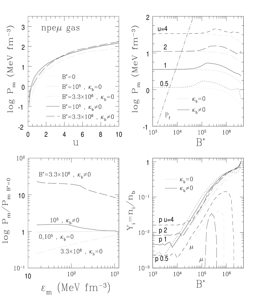
Figure 4:

Figure 5:

Figure 6:

Figure 7:

References

• (1) Abrahams, A. M., & Shapiro, S. L. 1991, ApJ, 374, 652
• (2) Boguta, J. & Bodmer, A. R. 1977, Nucl.Β Phys.,Β A292, 413
• (3) Bjorken, J., & Drell, S. 1964, in Relativistic Quantum Mechanics (McGraw-Hill: New York)
• (4) Blandford, R.D. & Hernquist, L., 1982, J. Phys. C: Solid State Phys., 15, 6233
• (5) Boucquet, M., Bonozzola, S., Gourgoulhon, E., & Novak, J. 1995 Astron. & Astrophys. 301, 757
• (6) Canuto, V., & Ventura, J. 1977, Fund. Cosmic Phys., 2, 203
• (7) Cardall, C.Y., Broderick, A., Prakash, M. & Lattimer, J.M. 1999, to be published
• (8) Chakrabarty, S. 1996, Phys. Rev. D54, 1306
• (9) Chakrabarty, S., Bandyopadhyay, D., & Pal, S. 1997 Phys. Rev. Lett. 78, 2898
• (10) Duncan, R.C. & Thompson, C. 1992, ApJ, 392, L9
• (11) Duncan, R.C. & Thompson, C. 1996, ApJ, 469, 764
• (12) Ellis, J., Kapusta, J. & Olive, K. A. 1991, Nucl.Β Phys.Β B348, 345
• (13) Fushiki, I., Gudmundsson, E.H., & Pethick, C. J. 1989, ApJ, 342, 958
• (14) Fushiki, I., Gudmundsson, E.H., Pethick, C. J., & Yngvason, J. 1992, Ann. Phys., 216, 29
• (15) Glendenning, N. K. 1982, Phys.Β Lett.Β 114B, 392
• (16) Glendenning, N. K. 1985, Astrophys.Β J.Β 293, 470
• (17) Glendenning, N.K. & Moszkowski, S.A. 1991, Phys. Rev. Lett., 67, 2414
• (18) Horowitz, C.J., & Serot, B.D. 1981, Nucl. Phys. A368, 503
• (19) Itzykson, C., & Zuber, J.-B. 1980, Quantum Field Theory, (McGraw-Hill: New York)
• (20) Johnson, M.H & Lippman, B.A. 1950, Phys. Rev. 77, 702
• (21) Kapusta, J. & Olive, K. A. 1990, Phys.Β Rev.Β Lett.Β 64, 13
• (22) Knorren, R., Prakash, M. & Ellis, P.J. 1995, Phys. Rev., C52, 1855
• (23) Kouveliotou. C. et al., 1998, Nature, 393, 235
• (24) Lai, D. & Shapiro, S. 1991, ApJ, 383, 745
• (25) Landau, L.D., Lifshitz, E.M., & PitaevskiΔ­, L.P. 1984, Electrodynamics of Continuous Media 2nd ed. (New York: Pergamon)
• (26) Lattimer, J.M., Pethick, C.J., Prakash, M. & Haensel, P. 1991, Phys. Rev. Lett. 66, 2701
• (27) Melatos, A. 1999, ApJ, 519, L77
• (28) MΓΌller, H., & Serot, B.D. 1996, Nucl. Phys., A606, 508
• (29) Paczynski, B. 1992, Acta Astron., 42, 145
• (30) Prakash, M., Bombaci, I., Manju Prakash, Ellis, P.J., Lattimer, J.M., & Knorren, R. 1997, Phys. Rep. 280, 1
• (31) Prakash, M., Prakash Manju, Lattimer, J.M. & Pethick, C.J. 1992, ApJ, 390, L77
• (32) RΓΆgnvaldsson, Fushiki, I., Gudmundsson, E. H., C. J. Pethick, & Γ–. E., Yngvason, J., ApJ, 416, 276.
• (33) Schaffner, J. & Mishustin, I.N. 1996, Phys. Rev., C53, 1416
• (34) Sumiyoshi, K. & Toki, H. 1994, Astrophys.Β J.Β 422, 700
• (35) Thompson, C. & Duncan, R.C. 1995, MNRAS, 275, 255
• (36) Thompson, C. & Duncan, R.C. 1996, ApJ, 473, 322
• (37) Thorlofsson, A., RΓΆgnvaldsson, Γ–. E., Yngvason, J., & Gudmundsson E. H. 1998, ApJ, 502, 847
• (38) Weber, F. & Weigel, M. K. 1989, Nucl.Β Phys.,Β A505, 779
• (39) Y. F. Yuan, Y. F. & Zhang, J. L. 1999, ApJ, 525, 920
• (40) Zimanyi, J. & Moszkowski, S.A. 1990, Phys. Rev. C42, 1416;
β€”β€”β€”β€”- 1992, Phys. Rev. C45, 844
TABLE 1
NUCLEON-MESON COUPLING CONSTANTS
Model $n_{s}$ $-B/A$ $M^{*}/M$ $K_{0}$ $a_{\mbox{\tiny sym}}$ $g_{\sigma_{N}}/m_{\sigma}$ $g_{\omega_{N}}/m_{\omega}$ $g_{\rho_{N}}/m_{\rho}$ $b$ $c$
HS81 0.148 15.75 0.54 545 35.0 3.974 3.477 2.069 0.0 0.0
GM1 0.153 16.30 0.70 300 32.5 3.434 2.674 2.100 0.002947 $-0.001070$
GM2 0.153 16.30 0.78 300 32.5 3.025 2.195 2.189 0.003478 0.01328
GM3 0.153 16.30 0.78 240 32.5 3.151 2.195 2.189 0.008659 $-0.002421$
ZM 0.160 16.00 0.86 225 32.5 2.736 1.617 2.185 0.0 0.0