Toy model of obscurational variability in active galactic nuclei

Abstract

We propose an explanation of the variability of AGN based on a cloud model of accretion onto a black hole. These clouds, present at a distance of 10-100 $r_{Schw}$, possibly come from the disrupted innermost disk and they can partially obscure the central X-ray source due to their extreme Compton optical depth. We consider the implications of this scenario using a toy model of AGN spectra and support the results with full radiative transfer computations from the codes titan and noar. We show that small random rearrangements of the cloud distribution can happen on timescales of the order of $10^{2}-10^{6}$ s and may lead to relatively high variability amplitude in the X-ray band if the mean covering factor is large. The normalized variability amplitude in the UV band is either the same as in the X-ray band, if the contribution from the dark sides of the clouds to the UV band is negligible, or it is smaller. The X-ray spectrum should basically preserve its spectral shape even during the high amplitude variability, within the frame of our model.

1 Introduction

Radio-quiet active galactic nuclei (AGN) are well known to be variable in the X-ray band since early observations by EXOSAT (e.g. Lawrence et al. 1987, McHardy & Czerny 1987, Green, McHardy & Lehto 1993). The combined study of both the X-ray spectra and variability offer the most direct insight into the structure of accretion flow onto the black hole which powers the AGN (for a review, see Mushotzky, Done & Pounds 1993).

The variability trends have been extensively studied in various spectral bands (e.g. Ulrich, Maraschi & Urry 1997, Peterson et al. 1998). Generally, more luminous objects are less variable both in X-rays (Nandra et al. 1997 and the references therein) and in the optical/UV band (Ptak et al. 1998, Giveon et al. 1999).

Multi-wavelength studies showed that this variability is surprisingly complex. In the X-ray band, most of AGN vary but individual sources display various spectral trends with the brightening of the source (e.g. Ciliegi & Maccacaro 1997, George et al. 1998, Nandra et al. 1997). The correlated variability between different energy bands is also difficult to interpret (e.g. Nandra et al. 1998 for UV and X-ray connection in NGC 7469).

The question appears to be whether this observed variability is entirely intrinsic, i.e. related to strongly non-stationary release of gravitational energy of the in-flowing matter, or is caused, at least partially, by the effect of variable obscuration towards the nucleus.

Partial covering models were popular mostly at the beginning of spectral studies in the X-ray band (e.g. Mushotzky et al. 1978, Matsuoka et al. 1986). Recently, Seyfert 1 galaxies and QSOs are modeled through an accretion disk, with X-ray emission coming either from the disk corona or from the disrupted innermost part of the disk (e.g. Loska & Czerny 1997 and the references therein).

However, occasionally, the problem was revived. An eclipse by a cloud was successfully considered as a model for the faint state of MCG-6-30-15 (McKernan & Yaqoob 1998, Weaver & Yaqoob 1998) and it may be a possible cause of the $K_{\alpha}$ line profile variability in NGC 3516 (Nandra et al. 1999). In the case of the variability of Narrow Line Seyfert 1 galaxies (e.g. Boller et al. 1997 for IRAS 13224-3809; Brandt et al. 1999 for PHL 1092) it was suggested that the observed huge amplitudes are hard to explain directly through a variable energy output, and instead, partial covering and/or relativistic erratic beaming may be necessary. It is interesting to note that the partial covering mechanism may also apply to similarly variable galactic sources (Brandt et al. 1996 for Cir X-1). Obscuration events are also sometimes invoked to explain the variations of the Broad Emission Lines in Seyfert galaxies - for example, a spectacular change of morphological type from Seyfert 2 to Seyfert 1 of the galaxy NGC 7582 (Aretxaga et al. 1999) was interpreted as due to an obscuration event by a distant cloud (Xue et al. 1998). Finally, there is a large amount of partially ionized material lying along the line of sight to the nucleus which manifests itself as a warm absorber (cf. Reynolds 1997). Variability in absorption edges can either be due to a variation of the ionisation state of the absorber or to obscuration by clouds passing through the line of sight.

Although there are now strong suggestions that the accretion flow proceeds predominantly through a disk the physics of the innermost part of the flow is highly uncertain. As the inner regions of a standard Shakura-Sunayev (1973) disk are thermally and viscously unstable in an AGN owing to the large radiation pressure, the disk is frequently supposed to be disrupted. It may form a hot, optically thin, quasi spherical ADAF (advection-dominated accretion flow; Narayan & Yi 1994, and many subsequent papers), or it may proceed in the form of thick clouds (Collin-Souffrin & al 1996, hereafter referred as Paper I). Such clouds might be optically thick, unlike clouds optically thin for electron scattering which form spontaneously as a result of thermal instability in X-ray irradiated cold gas and coexist in equilibrium with the surrounding hot optically thin gas (Krolik 1998, Torricelli-Ciamponi & Courvoisier 1998). Such clouds provide significant mass flux and they are not easily destroyed (see Sect. 4 in Paper I); they may even condensate under favorable conditions but the criterium for evaporation or condensation depends on the assumed heating mechanism (see Różańska & Czerny 1999 and the references therein). In another model (Celotti, Fabian & Ress, 1992, Sivron & Tsuruta 1993, Kuncic, Celotti & Rees 1996) very dense blobs confined by magnetic pressure, optically thin to scattering and thick to free-free absorption, form in a spherical relativistic flow.

Within the frame of the cloud scenario, obscuration events are expected. If clouds have a column density in excess of $\sim 10^{25}$ cm^-2, the obscuration events would be observed as variability, whatever the size of the clouds (smaller or larger than that of the central source).

In the present paper we discuss the possibility of explaining, at least partially, the variability phenomenon by variable obscuration. We consider the case of random variability due to the statistical dispersion in location of clouds along the line of sight for a constant covering factor. We provide simple analytical estimates of the mean spectral properties, timescales and variability amplitude of AGN, and we support them with computations of radiative transfer done with the use of the codes titan (Dumont, Abrassart & Collin 1999) and noar (Abrassart 2000).

2 Model

2.1 Cloud model scenario

Accretion flow onto a black hole proceeds most probably down to a hundred Schwarzschild radiiin the form of an accretion disk. Closer in, the relatively cool accretion disk is disrupted and replaced with a mixture of still cold optically thick clumps and hot gas which is responsible for hard the X-ray emission. The cold clumps may not be constrained to the equatorial plane but, under the influence of radiation pressure, may have a quasi-spherical distribution. We envision this general picture in Fig. 1 (see also Fig. 1 in Karas et al. 1999). Such a scenario offers an interesting possibility for explaining the observed spectra of AGN. Although other geometries of the innermost part of accretion flow are not excluded, we concentrate on exploring this particular model.

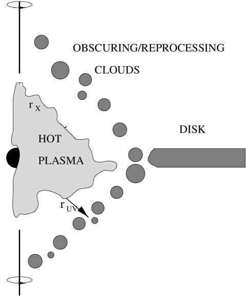
Figure 1: A fantasy view of the cross-section through the central region of the accretion flow into a black hole. In the paper, we idealize this geometry assuming a spherically symmetric distribution of the clouds at a characteristic radius and a spherical shape for the hot central plasma.

The mechanism of disk disruption is unknown and therefore the dynamics of the cloud formation process cannot be described. The formation of the hot medium is also not well understood, although it must proceed in some way through cloud evaporation. Therefore we have to resort to a phenomenological parameterization of the cloud distribution and the hot gas geometry. A realistic approach to the cloud model would require a large number of arbitrary parameters reproducing the radial structure and the departure from spherical symmetry. However, the most essential properties of the model can be studied within the frame of a much simpler model.

In the present paper we follow the geometry adopted by Czerny & Dumont (1998) for their model C (see their Fig. 2).

We assume that the hot medium forms a central spherical cloud of radius $r_{X}$. It is characterized by its Thomson optical depth, $\tau$, and by its electron temperature, $T_{e}$. Those two parameters uniquely determine the Compton amplification factor $A(\tau,T_{e})$ of the hot medium.

The cold clouds are located at a typical distance $r_{UV}$ from the center and their distribution is characterized by the covering factor $\Omega/4\pi$. They reprocess the X-ray emission from the hot medium. A fraction of the incident X-ray photons is backscattered, but most of the photons are absorbed. This absorbed radiation is mostly reemitted in UV by the bright side of the clouds, but a fraction is leaking through the dark side. The photons reemitted by the bright side provide seed photons for Comptonization by the central hot medium.

The bremsstrahlung emission from the central comptonizing cloud (CCC) does not significantly contribute to the energy budget, for all the parameters we considered. In this model the prime movers of the engine are the X-rays, in the sense that they are produced in a region (of radius $r_{X}$) close to the black hole, and they drive the reprocessed UV emission further away. But the intrinsic emission of the hot plasma being small, it basically acts as a reservoir of energy, used to upscatter a fraction of the reprocessed UV photons. As the thick clouds can be highly reflective in the UV, this “recycling” of photons can be very efficient when $\Omega/4\pi$ is large. The efficiency of the subsequent production of X-rays is also high if the scattering probability of UV photons, determined by the optical depth of the hot plasma $\tau$ and the relative geometrical cross-section $(r_{X}/r_{UV})^{2}$, is not too low. This geometry may thus imply a stronger coupling between the two emission regions than the alternative disk/corona configuration, where about half of the comptonized power escapes directly.

2.2 Radiative transfer computations

An accurate description of the radiative coupling between the hot plasma and the relatively cold clouds requires complex computations of radiation transfer. In particular, the emission from the bright side of the clouds strongly depends on the ionization state of the gas.

We calculate the emission from the bright and dark sides of the clouds in the optical/UV range using the radiative transfer code titan of Dumont, Abrassart & Collin (1999) for Compton thick media. The same code was used by Czerny & Dumont (1998) over the entire optical/X-ray range. However, in the present version we pay more attention to an accurate description of the hard X-ray transfer within the hot plasma and within the surface layers of clouds, therefore we use the Monte Carlo code noar of Abrassart (2000).

In order to obtain a single spectrum model, both codes - titan and noar - have to be used in a form of iterative coupling, as described in detail by Abrassart (2000). The method is very time consuming, so for the purpose of the present studies of variability, we develop a simple analytical toy model which allows estimates of the observed trends in a broad range of parameters. Therefore, we use the numerical results as a test of the toy model and as a source of information about physically reasonable mean quantities such as the frequency-averaged albedo, the fraction of radiation lost by the dark sides of the clouds, etc.

2.3 Toy model

In numerical simulations both the scattered and the reemitted component form a complex reflected spectrum with a shape mostly determined by the ionization parameter

$$\xi=4\pi F_{inc}/n,$$ (1)

where $F_{inc}$ is the incident radiation flux and $n$ is the number density of a cloud, although the shape of the observed spectrum is even more influenced by the value of the cloud covering factor. In Fig. 2 we show the ratio of the radiation reflected/reemitted by the bright side of the irradiated cloud for a value of the ionization parameter $\xi$ equal 300 and a power law spectrum proportional to $\nu^{-1}$ (the ratio depends little on the density and column density, provided the latter is larger than 10²⁵ cm^-2, for a range of density between 10¹⁰ and 10¹⁵ cm^-3). As we see, the true absorption is very low below the Lyman discontinuity, even for such a relatively low $\xi$, the reflectivity is very close to unity, and the absorbed and thermalized X-ray flux emitted in the UV creates an excess seen in UV/soft X-rays.

Figure 2: The ratio of the broad band reprocessed spectrum (i.e. reflected and reemitted) to the incident power law spectrum in the plane parallel geometry for the value of the ionization parameter $\xi=300$ (see text).

Therefore, due to reprocessing by cold clouds, the initial almost power law distribution of photons produced by Comptonization is replaced by a still broad hard X-ray component and a much more peaked UV/soft X-ray component. The X-ray component is produced by subsequent scattering of photons within the hot cloud, thus forming basically a power law spectral shape with a high energy extension and a slope determined by the properties of the hot cloud ($\tau,T_{e}$). Cloud emission is closer to a black body and the maximum of the spectrum is mostly determined by the temperatures of the dark and bright sides of the clouds.

Here, for the purpose of an analytical analysis, we simplify this distribution.

The entire optical/UV/X-ray range is schematized by defining two representative energy ranges: soft (UV) or hard (X-ray), with mean energies $E_{UV}$ and $E_{X}$. The exact values of those energies are not essential as they do not enter as model parameters through conservation laws (see Appendix A).

We reduce the description of radiative transfer to coefficients which determine the efficiency of the change of an X-ray photon into a UV-photon, and the reverse.

We reduce the photon-frequency-dependent albedo, describing the efficiency of reflection of X-ray photons, to some energy-integrated value, $a$. We introduce a frequency-averaged fraction of the X-ray luminosity, $\beta_{d}$, which leaks through the dark side of the clouds in the form of UV emission instead of being reemitted by the bright side.

We also simplify the description of Comptonization by using a mean Compton amplification factor independent of the energy of the input soft photon.

Variability properties are related to the mean spectral shape of an AGN. Therefore we have to introduce a relation between the cloud distribution and the observed spectral shape before discussing the variability itself.

2.3.1 Mean properties of the cloud distribution

We can formulate the conditions for the stationary situation, in which the escape of the photons from the system should be compensated by the production of new photons at the expense of the energy flux supplied to the hot cloud. Noting $C=\Omega/4\pi$ and $\gamma=\tau/(1+\tau)(r_{X}/r_{UV})^{2}$, the fate of a UV photon at every travel across the region is determined by the following probabilities:

$$(1-\gamma)(1-C)=P_{esc}^{UV}$$ (2)

$$(1-\gamma)C=P_{refl}^{UV}$$ (3)

$$\gamma=P_{ups}^{UV},$$ (4)

where $P_{esc}^{UV}$ is the probability of escape from the system, $P_{refl}^{UV}$ is the probability of reflection by the clouds and $P_{ups}^{UV}$ describes the probability of conversion into an X-ray photon due to the Compton upscattering.

For an X-ray photon we have the following probabilities:

$$1-C=P_{esc}^{X}$$ (5)

$$aC=P_{refl}^{X}$$ (6)

$$(1-\beta_{d})(1-a)C=P_{abs}^{X}$$ (7)

$$(1-a)C\beta_{d}=P^{UV}_{dark},$$ (8)

where $P_{esc}^{X}$ is the escape probability, $P_{refl}^{X}$ is the probability of reflection by the clouds, $P_{abs}^{X}$ describes the probability for an X-ray photon to be absorbed by the clouds and reemitted in the form of UV radiation through the bright side, while $P^{UV}_{dark}$ describes the probability of absorption of an X-ray photon and subsequent reemission in the form of UV radiation through the dark side.

We have to compensate for the loss of UV photons with new UV photons created in a sequence of events: upscattering a fraction of UV photons by the hot plasma and creating X-rays, absorption of X-rays by the cold clouds, and reemision of this energy in the form of UV photons (see Appendix A):

$${(P_{esc}^{UV}+P_{ups}^{UV})(P_{esc}^{X}+P_{abs}^{X})\over P_{ups}^{UV}P_{abs}^{X}}=A(\tau,T_{e}).$$ (9)

The stationarity can be clearly achieved only if $A$ is greater than unity.

In the present formulation of the model we assumed that the emission from the dark sides of the clouds is provided by X-ray photons. We could instead assume that it is mostly the leaking of UV photons diffusing through an optically thick cloud which powers the dark side emission. This would mean adding the factor $(1-\beta_{d})$ to the left side of Eq. 3, adding a new equation to the set formulated for a UV photon: $(1-\gamma)C\beta_{d}=P_{dark}^{UV}$, while putting $\beta_{d}=0$ in Eq. 8, and dropping Eq. 7 in the set formulated for an X-ray photon. These two approaches are almost equivalent unless $\gamma$ is very close to 1, corresponding to a change of all UV photons into X-rays.

The ratio of the intrinsic bolometric luminosities of these two spectral components inside the region is given by (see Appendix A)

$$\left({L_{X}\over L_{UV}}\right)_{int}={P_{esc}^{UV}+P_{ups}^{UV}\over P_{abs}^{X}}={A\gamma\over 1-aC}.$$ (10)

This equation shows that for a given system (specified by C, a, and $\gamma$), $L_{X}\over L_{UV}$ is upper bounded by the limited heat supply to the central comptonizing cloud.

2.3.2 Mean properties of the observed spectrum

The observed spectrum is not identical to the spectrum inside the production region since the escape probability for UV and X-ray radiation differs by a factor of $(1-\gamma)$ (compare Eqs. 2 and 5), and X-rays transformed into dark emission additionally change the relative proportions.

The observed ratio of the bolometric luminosities in the two components is therefore given by:

$$\left({L_{X}\over L_{UV}}\right)_{obs}={\left({L_{X}\over L_{UV}}\right)_{int}(1-C)\over(1-C)(1-\gamma)+\left({L_{X}\over L_{UV}}\right)_{int}\beta_{d}(1-a)C}.$$ (11)

This formula simplifies considerably if the contribution of the dark sides of the clouds is neglected:

$$\left({L_{X}\over L_{UV}}\right)_{obs}=\left({L_{X}\over L_{UV}}\right)_{int}{1\over(1-\gamma)}$$ (12)

This is true if the clouds are very thick, as then their dark side temperature is low and the radiation flux peaks in the optical band.

It is worth noting that the observed luminosity ratio can be expressed independently of $\gamma$ or $\beta_{d}$:

$$\left({L_{X}\over L_{UV}}\right)_{obs}=\frac{A\,\left(-1+C\right)}{1+a\,\left(A-1\right)\,C-A\,C}.$$ (13)

2.4 Model of stochastic variability

We can consider two variability mechanisms expected within the frame of the cloud model and of the geometry of the inner flow.

Random variability at a certain level is always expected since the cloud distribution is assumed to be uniform (spherically symmetric) in a statistical sense. Even without any systematic evolutionary changes of the covering factor $C$, our view of the nucleus will undergo variations due to the instantaneous covering factor of the side of the distribution facing the observer.

Systematical trends may also show up if there is a systematic evolutionary change in the mean covering factor, $C$.

2.4.1 Random variability amplitude

The most basic parameter of the variability is its amplitude at a given wavelength. In order to reproduce it within the frame of the cloud model we have to assume that clouds can have some random velocities which do not change the mean covering factor but change randomly the number of clouds which occupy the hemisphere just facing us.

If we have $N$ clouds, half of them on average occupy the front hemisphere and the dispersion around that mean value would be given by

$$\delta(N/2)=\sqrt{N/2}$$ (14)

so the covering factor as seen by us also displays variations with an amplitude

$$\delta C=C\sqrt{2/N}$$ (15)

Therefore the amplitude of variability of the observed X-ray emission is given by

$$\left({\delta L_{X}\over L_{X}}\right)_{obs}={C\sqrt{2/N}\over 1-C}.$$ (16)

High X-ray variability is achieved if the covering factor is high and the number of clouds is not too large.

The UV variability depends again on the optical depth and the contribution of the dark sides predominantly to the UV or optical band.

If dark sides of the clouds are too cool to radiate in the UV, the variability amplitude is given by the same formula as for X-rays

$$\left({\delta L_{UV}\over L_{UV}}\right)_{obs}={C\sqrt{2/N}\over 1-C}.$$ (17)

However, if the dark sides contribute to the UV we have

$$\left({\delta L_{UV}\over L_{UV}}\right)_{obs}={C\sqrt{2/N}[(1-\gamma)(1-aC)-\gamma A(1-a)\beta_{d}]\over(1-\gamma)(1-C)(1-aC)+\gamma A(1-a)C\beta_{d}}$$ (18)

which reduces the UV relative amplitude.

Such normalized variability amplitudes depend on the number of clouds, $N$, constituting the UV emitting region. This means that an additional free parameter is involved.

The normalized variability amplitudes can be determined observationally. Studies of variability provide us either with the rms value in a given spectral band, or just with a typical value of the variability factor. Quoted rms values can be directly identified with our normalized amplitude. If instead only a variability factor is given, we can understand it as statistical variations at 2 standard deviation level. This means that we actually observe variability of a factor ${\cal A}$ when the luminosity changes from $L_{X}-2\delta L_{X}$ to $L_{X}+2\delta L_{X}$.

Therefore this variability factor can be expressed as

$${\cal A}=L_{X}(max)/L_{X}(min)={1+2\left({\delta L_{X}\over L_{X}}\right)_{obs}\over 1-2\left({\delta L_{X}\over L_{X}}\right)_{obs}}.$$ (19)

We can also define the ratio $R$ as the ratio of the normalized variability amplitudes in the X-ray band and in the UV band:

$$R={\left({\delta L_{X}\over L_{X}}\right)_{obs}\over\left({\delta L_{UV}\over L_{UV}}\right)_{obs}}.$$ (20)

Such a ratio does not depend on the number of clouds, $N$, constituting the UV emitting medium. Therefore this ratio is fully determined by the parameters of our toy model.

2.4.2 Random variability timescales

The random variability we consider results from the clouds passing through our line of sight to the central source. On the one hand, each passing cloud produces an eclipse phenomenon. On the other hand, the dispersion in the cloud velocities, due to even a small dispersion of the distances from the gravity center, results in variations of the cloud distribution, as described in Sect. 2.4.1.

Let us estimate a representative duration $t_{dip}$ of an obscuration event. This is determined by the size and velocity of a cloud as well as the size of the X-ray source and the entire region involved. The cloud velocity is of the order of the keplerian velocity so it is determined by the mass of the black hole (or its gravitational radius) and $r_{UV}$. A typical size of a cloud is given simply by the number of clouds, the radius $r_{UV}$ and the covering factor, if there is at most one cloud in the line of sight, i.e. clouds are not overlapping.

The mean number of clouds in a line of sight is of the order of unity (cf Appendix B) so we get the typical cloud size:

$$r_{cl}^{2}\sim{C\over N}r_{UV}^{2}.$$ (21)

Here we have ignored numerical factors of the order of $\pi$, since this expression, and the following formulae, serve only as an order of magnitude estimate.

Since the clouds are ten or more times smaller than the region involved, the fastest variation corresponds to an ingress or an egress from a single eclipse

$$t_{min}\sim{r_{Schw}\over c}\sqrt{{4C\over N}({r_{UV}\over R_{Schw}})^{3}}.$$ (22)

Typical random rearrangement of the cloud distribution will proceed on a dynamical timescale connected with Keplerian motion

$$t_{d}\sim{r_{Schw}\over c}\sqrt{({r_{UV}\over r_{Schw}})^{3}}.$$ (23)

If the cloud distribution covers a range of radii, the longest timescale involved will be given by $t_{d}$ at the outer edge of the cloud distribution.

2.4.3 Variations of the covering factor in the toy model

This kind of variability is more complex to study since variations in the covering factor lead not only directly to variations of $L_{X}$ and $L_{UV}$ but also result in a change of the mean number of clouds along the line of sight, and, under an assumed constant total luminosity, in a change of the ionization state of the clouds, i.e. albedo. Such trends can only be studied by solving the radiative transfer equation for a sequence of models, which we postpone to a future paper.

2.5 Relation between toy model parameters and the ionization parameter

The spectral features in X-ray band allow us to have an insight into the ionization state of the reprocessing medium. This ionization state is mostly determined by the value of the ionization parameter $\xi$. Since we frequently have some direct estimates of this parameter, it is interesting to relate this parameter to the parameters of our toy model. It will allow for simple estimates of those parameters through the quantities which can be estimated on the basis of observational data. That way, we can judge to some extent the applicability of the model.

For a bolometric luminosity of an object, $L$, the incident flux determining the ionization parameter, $\xi$, (Eq.1) in the case of the quasi-spherical distribution of clouds is:

$$F_{inc}={L\over r_{UV}^{2}},$$ (24)

where $n$ is the number density of the clouds and $r_{UV}$ is the representative distance of a cloud from the black hole.

The most convenient form of relating the number of clouds to the ionization parameter and other observables is through the explicit dependence on the covering factor and the column density of the clouds, $N_{H}$. We can derive the appropriate formula knowing that the typical size of the cloud $r_{cl}$ is related to $N$, the covering factor and the characteristic radius of the cloud distribution (see Eq. 21).

The obtained relation

$$N\sim L^{2}CN_{H}^{-2}r_{UV}^{-2}\xi^{-2}.$$ (25)

indicates that the number of clouds scales with the square of the luminosity to the Eddington luminosity ratio, $R_{Edd}$, if $N_{H}$, $\xi$ and $r_{UV}$ (expressed in Schwarzschild radii) are similar in all objects. It means that high luminosity, low covering factor objects should be the least variable. If this estimate of the number of clouds is inserted into Eqs. 17 and 16 we see that we do not expect a direct scaling with the central mass of the black hole or bolometric luminosity. The very weak trends between the UV variability and the bolometric luminosity observed in the data (Paltani & Courvoisier 1997, Hook et al. 1994) might be caused by some secondary coupling between the mass of the black hole and the model parameters.

The size and the number of clouds is constrained by the dimension of the emission region, as the volume filling factor has to be smaller than unity:

$${Nr_{cl}^{3}\over r_{UV}^{3}}\ll 1,$$ (26)

or:

$$N_{H}\xi\ r_{UV}\ L^{-1}\ll 1.$$ (27)

One can now illustrate the properties of the cloud model with some numbers.

Expressing the mass of the black hole in 10⁸M_⊙, $R_{Edd}$ in 10^-1, $N_{H}$ in 10²⁶ cm^-2, $\xi$ in 10³ and $r_{UV}$ in 10 $r_{Schw}$, one gets, using Eqs. 21 and 25:

$$r_{cl}\sim 2\times 10^{12}N_{26}\xi_{3}\left({r_{UV}\over 10r_{Schw}}\right)^{2}M_{8}\left({R_{Edd}\over 0.1}\right)^{-1}{\rm cm}$$ (28)

$$n_{H}\sim 5\times 10^{13}\xi_{3}^{-1}\left({r_{UV}\over 10r_{Schw}}\right)^{-2}M_{8}^{-1}{R_{Edd}\over 0.1}\ {\rm cm}^{-3}$$ (29)

$$N\sim 10^{4}CN_{26}^{-2}\xi_{3}^{-2}\left({r_{UV}\over 10r_{Schw}}\right)^{-2}\left({R_{Edd}\over 0.1}\right)^{2},$$ (30)

and the condition on the filling factor:

$$10^{-3}CN_{26}\xi_{3}{r_{UV}\over 10r_{Schw}}\left({R_{Edd}\over 0.1}\right)^{-1}\ll 1,$$ (31)

Clouds with such properties could form for instance as broken pieces of the inner accretion disk.

Using Eqs. 25 and 16 the X-ray variability amplitude is:

$$\left({\delta L_{X}\over L_{X}}\right)_{obs}\sim{\sqrt{C}\over(1-C)}L^{-1}N_{H}r_{UV}\xi$$ (32)

It is maximum for a covering factor equal to 0.5, corresponding to two clouds along the line of sight, on average.

Using the same notation as in Sect. 2.5, the X-ray variability amplitude is:

$$\left({\delta L_{X}\over L_{X}}\right)_{obs} \sim \sqrt{2}\times 10^{-2}{\sqrt{C}\over(1-C)}N_{26}\xi_{3}$$

$$\left({R_{Edd}\over 0.1}\right)^{-1}{r_{UV}\over 10r_{Schw}}.$$

and the time scale of the variability, using Eq. 22:

$$t_{dip}\sim 10^{2}\ N_{26}\ \xi_{3}\left({R_{Edd}\over 0.1}\right)^{-1}M_{8}\ {\rm sec}$$ (34)

We see that a large variability amplitude in a very small time scale is easily obtained in this model.

We cannot expect, however, that the overall variability properties of AGN may be explained by eclipsing clouds all being at the same distance and having the same radius. Actually, any more realistic picture would require clouds to occupy a range of radii.

3 Results

The complete toy model of the stationary distribution of clouds depends on four parameters: the covering factor, $C$, the probability of upscattering a $UV$ photon into an X-ray photon, $\gamma$, the X-ray albedo of the bright side of the clouds, $a$, and the fraction of the X-ray radiation leaking through the dark side of the clouds in the form of $UV$ radiation, $\beta_{d}$. These four values determine the Compton amplification factor of the hot plasma, $A$, through the conservation law given by Eq. 9. In full radiative transfer numerical models the number of free parameters is the same: $C$, $r_{X}/r_{UV}$, $r_{X}$, and the hot plasma parameters $\tau$ and $T_{e}$. Fortunately the number density and the column density of the cloud system play a small role. However the freedom in modeling is considerable. Therefore, in order to study the cases which are of direct interest to observed AGN, we consider first in some detail the mean Seyfert spectrum in order to fix some of these parameters to be used in most of our further considerations.

3.1 Toy model of the mean properties of Seyfert 1 galaxies

Figure 3: The dependence of the Compton amplification factor on the hot plasma temperature, $T_{e}$, for the optical depth of the plasma adjusted for each temperature to fix the hard X-ray slope index at 0.9. The soft photon temperature is 50 eV.

The broad band spectra of Seyfert 1 galaxies are relatively well known. Most objects have an intrinsic hard X-ray slope of about $\sim 0.9$ if the spectra are corrected for the reflection component (Nandra & Pounds 1994). However, determination of the shape of the high energy tail of the spectrum of a single object poses a considerable problem. Relatively strong constraints on the spectrum extension for typical Seyfert galaxies can be only achieved through the analysis of composite spectra, i.e. summed spectra of a number of objects. Such a composite spectrum was published by Gondek et al. (1996) on the basis of combined Ginga/OSSE data for 7 Seyfert 1 galaxies. We use this spectrum to reduce the degrees of freedom in our models.

3.1.1 Compton amplification factor

A relatively low dispersion in the observed X-ray slopes of Seyfert galaxies around the mean value 0.9 allows us to estimate the characteristic Compton amplification factor. We use for this purpose the Monte Carlo results of Janiuk, Życki & Czerny (2000).

The Comptonization process by a hot spherical cloud depends on two parameters: optical depth of the cloud, $\tau$, and electron temperature, $T_{e}$, and leads to a broad range of X-ray slopes. However, for each value of $T_{e}$ we can find an optical depth which gives a spectral slope of 0.9. Therefore we finally obtain the value of the Compton amplification factor as a function of $T_{e}$ only. The corresponding plot is shown in Fig.  3.

Determination of the value of $T_{e}$ from the observed high energy cutoff in the X-ray spectra is rather uncertain. Gondek et al. (1996) give the value of 260 keV for the combined Seyfert 1 spectrum from the Ginga/OSSE data. Fortunately, the dependence of $A$ on $T_{e}$ is weak. This is not surprising since both the spectral slope and the Compton amplification factor are mostly determined by the value of the Compton parameter $y$.

Adopting Te = 260 keV, we fix the value of the Compton amplification factor $A=4.0$ in further considerations (Fig. 3). It reduces the number of free parameters of our toy model to 3.

3.1.2 Expected trends in stationary parameters

Fixing the value of the Compton amplification factor leads to a relation between the original model parameters: $C$, $a$, $\beta_{d}$ and $\gamma$. It leaves a choice of 3 parameters out of 4, as basic independent model parameters. We analyse the relation in order to make the most convenient choice. We also study the dependence of the predicted luminosity ratios on our selected set of parameters.

Negligible dark side contribution

We consider first the case of negligible contribution of the dark sides of the clouds to the UV spectrum, due to their large optical depth ($\beta_{d}$ = 0).

The stationarity condition allows to express the probability of scattering by the hot cloud, $\gamma$, as the function of the X-ray albedo, $a$, and covering factor, $C$. We show this dependence in Fig. 4.

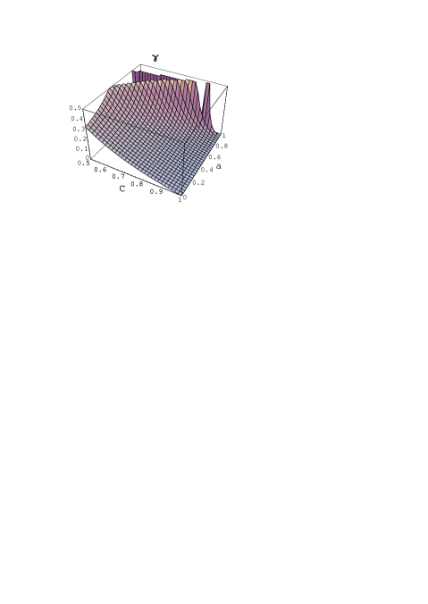
Figure 4: The dependence of the probability, $\gamma$, of UV photon upscattering by the hot plasma on the covering factor $C$ and the X-ray albedo $a$; fixed parameters are $\beta_{d}=0$ and $A=4$.

Factor $\gamma$ depends mostly on the covering factor but it also shows a trend to increase with the albedo (i.e. the ionization parameter). Only large values of the covering factor are allowed, as the optical depth of the hot cloud is small and the physical size of the X-ray region $r_{X}$ cannot be larger than $r_{UV}$ within the frame of our model. So $\gamma$ cannot be larger than $\tau$. It means that $C$ cannot be smaller than about 0.7 for $\tau=0.1$ although larger optical depth allow for smaller covering factors.

The role of the dark side contribution

The contribution from the dark sides of clouds may not, however, be negligible. Therefore, it is more appropriate to present the results by constraining the albedo. For a broad range of the ionization parameter $\xi$, the radiative transfer computations (Dumont & Abrassart 2000) show that the X-ray albedo, $a$, for partially ionized gas is about 0.5. If we use this constraint, it leaves us a choice of two independent parameters among $C$, $\gamma$ and $\beta_{d}$.

We plot the dependence of $\beta_{d}$ on the covering factor $C$ and the scattering probability $\gamma$ in Fig. 5. We see that $\beta_{d}$ should be relatively important for large covering factors and large $\gamma$. There is also a range of parameters (small $C$ and $\gamma$) for which the formally computed value of $\beta_{d}$ is negative (negative values are not plotted on the figure). Using $C$ and $\gamma$ as independent variables, we have to be aware of this unphysical range of parameters which depends to some extent on the adopted albedo. If we choose another set of two arbitrary parameters the unphysical range does not disappear.

The cross-section of Fig. 5 for constant $\beta_{d}$ produces $\gamma$ closely correlated to $C$. Such a relation for $\beta_{d}=0.2$ (it is a high value for the high optical thickness of our clouds, according to the transfer computations of Dumont & Abrassart, 2000) is rather similar to results for $\beta_{d}=0$.

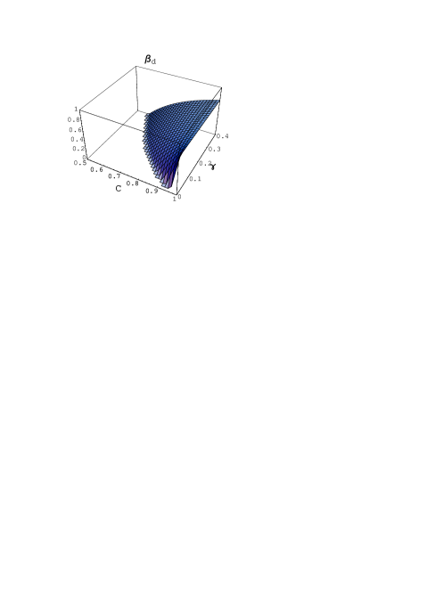
Figure 5: The dependence of the fraction, $\beta_{d}$, of absorbed X-ray flux to be reemitted by the dark sides of the clouds on the covering factor, $C$, and the probability of scattering by hot plasma, $\gamma$. Fixed parameters: $A=4$, $a=0.5$.

3.1.3 Expected trends in the luminosity ratios

The observed ratio of the X-ray to the UV luminosity depends only on the covering factor if the X-ray albedo and Compton amplification factor are fixed; it is not influenced by the second model parameter ($\gamma$ or $\beta_{d}$) within the frame of our toy model (see Eq. 13), in opposite to other quantities.

This quantity is one of the important observables, although in practice the determination of the $\left({L_{X}\over L_{UV}}\right)_{obs}$ ratio may not be easy because of extinction. It is also of major importance in all accretion models, so we have to study its dependence on the parameters which we usually fix, namely Compton amplification factor $A$ and X-ray albedo $a$.

In Fig. 6 we show the $\left({L_{X}\over L_{UV}}\right)_{obs}$ ratio. We see that this ratio mostly depends on the covering factor. For an albedo $a=0.15$ (cold matter) the X-ray luminosity starts to dominate the bolometric output only if the covering factor is smaller than 0.6. In the case of a larger albedo of partially ionized gas, $a=0.5$, the X-ray emission dominates the UV luminosity up to about $C=0.75$.

We see from this plot that $\left({L_{X}\over L_{UV}}\right)_{obs}$ is smaller than unity for the range of covering factors we consider. This is a very important characteristic of this model: it is able to account for a low X-ray to UV luminosity ratio without any ad-hoc hypothesis.

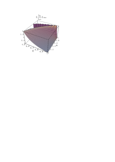
Figure 6: The dependence of the $\left({L_{X}\over L_{UV}}\right)_{obs}$ ratio on the covering factor, $C$, and the X-ray albedo, $a$. Fixed parameter: $A=4$.

Fig. 7 shows the dependence of $\left({L_{X}\over L_{UV}}\right)_{obs}/\left({L_{X}\over L_{UV}}\right)_{int}$ on the covering factor $C$ and $\gamma$ for $a=0.5$. This ratio, in contrast to $\left({L_{X}\over L_{UV}}\right)_{obs}$, depends on $\gamma$ as well, not just on the covering factor.

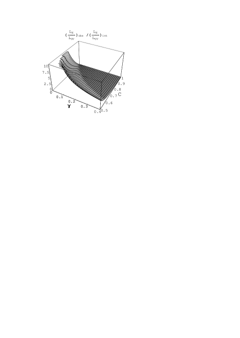
Figure 7: The dependence of$\left({L_{X}\over L_{UV}}\right)_{obs}/\left({L_{X}\over L_{UV}}\right)_{int}$ on the covering factor, $C$, and the probability of scattering by hot plasma, $\gamma$. Fixed parameters: $A=4$, $a=0.5$. The non-shaded part corresponds to $\beta_{d}<0$.

Over most of the allowed parameter space, $\left({L_{X}\over L_{UV}}\right)$ is slightly lower inside the clouds system than what is observed. It is also interesting to note that the X-ray to UV luminosity ratio seen outside the cloud system can be larger than this ratio determined inside the medium, or in other words that inside the medium the radiation field is softer than the observed spectrum. The effect is stronger towards small values of $\gamma$, but the parameter space where this happens is rather narrow, because the highest values happen where there are no physical solutions. Indeed, the energy losses through the dark sides of the clouds take negative values for a large range of covering factor and probability of scattering by the hot plasma (see Fig. 5).

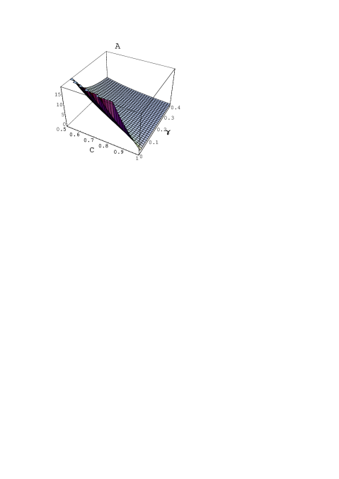
Figure 8: The dependence of the Compton amplification factor on the covering factor, $C$, and the probability of scattering by hot plasma, $\gamma$. Fixed parameters: a=0.5, $\beta_{d}=0$.

The reason for this can be more clearly seen on Fig. 8, for which we relaxed the A=4 assumption, but fixed $\beta_{d}$. This last parameter does not qualitatively change the behavior of the equilibrium amplification factor but simply forces it to higher values when it raises. One sees that fixing A defines a unique relation in the C,$\gamma$ plane, but that there are no solutions on either side of this line. By raising $\beta_{d}$, it is possible to find an equilibrium on the side where A is too high, but the side where A is not sufficient is clearly forbidden.

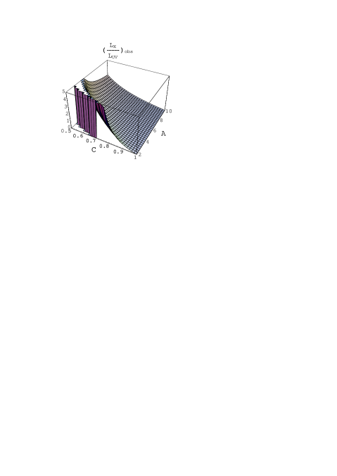
Figure 9: The dependence of the $\left({L_{X}\over L_{UV}}\right)_{obs}$ ratio on the covering factor, $C$, and Compton amplification factor, $A$. Fixed parameter: $a=0.5$.

The accuracy of the determination of the Compton amplification factor does not influence much the X-ray to UV luminosity ratio if the covering factor is large. This dependence is plotted in Fig. 9, for an X-ray albedo of one half. Higher albedos (i.e. ionization state) require higher covering factors, whatever the amplification factor, in order to keep a reasonably low X-ray to UV luminosity ratio.

3.1.4 Toy model for the Gondek et al. spectrum

We can now find model parameters which reproduce the shape of the mean Seyfert spectrum of Gondek et al. (1996). We need, for this purpose, the observed $({L_{X}\over L_{UV}})$ ratio, the X-ray albedo and the contribution from the dark sides $\beta_{d}$. Also the optical depth of the hot plasma (or its temperature) is required in order to obtain the relative size of the cloud distribution to the radius of the hot plasma, $r_{X}/r_{UV}$.

We have no accurate measurements of the X-ray to the UV bolometric luminosity ratio for this sample since the UV data are very sensitive to even minor absorption, and the extension of this spectral component into the EUV is difficult to incorporate into the bolometric luminosity of the soft component. The $\nu F_{\nu}$ fluxes measured at 1375 Å and 2 keV given by Walter & Fink (1993) can be used to make a rough estimate. Of the sources included in the combined Seyfert 1 spectrum by Gondek et al. (1996), two are heavily absorbed in the UV: MCG 8-11-11 and MCG-6-30-15 so they have to be rejected. The remaining five sources have the average ratio $\nu F_{\nu}$ at 1375 Å  to $\nu F_{\nu}$ at 2 keV about 14, with the highest value being $\sim 20$. Since the X-ray component is much broader, we have to apply a bolometric correction $K$ to it in order to roughly reproduce the broad band luminosity ratio. We assume $K=4$ so we obtain $(L_{X}/L_{UV})_{obs}=K/14=0.3$. This is only a rough estimate; the result of detailed analysis would depend significantly on the temperature of the $UV$ component.

Such an observed luminosity ratio can be used to estimate the parameters of the cloud distribution. Assuming the value of albedo for partially ionized matter $a=0.5$, $A=4$, $(L_{X}/L_{UV})=0.3$ and neglecting the contribution from the dark sides ($\beta_{d}=0)$ we obtain the covering factor $C=0.87$ and $\gamma$ equal 0.052 (for $a=0.3$, $\gamma$ is the same, and $C=0.91$). The value of $\gamma$ can be used to determine the $r_{X}/r_{UV}$ if we know the optical depth of the hot cloud. Taking the optical depth $\tau=0.1$ after Gondek et al. (1996) we obtain $r_{X}/r_{UV}=0.72$. However, observational determination of $\tau$ strongly depends on the (rather poor) accuracy of the determination of the high energy cut-off. Assuming a larger value of $\tau=0.3$ we obtain $r_{X}/r_{UV}=0.42$. We therefore see that we can determine reliably the parameter $\gamma$, but the factorization of its value between the physical size of the hot cloud and the optical depth is only weakly constrained by the details of the spectral shape.

Allowing for a relatively high ratio of energy leaking through the dark sides, $\beta_{d}=0.1$, we obtain: $C=0.93$, $\gamma=0.03$ which translates to $r_{X}/r_{UV}$ equal 0.55 for $\tau=0.1$ and 0.32 for $\tau=0.3$.

3.2 Random variability

Detailed observations of the variability pattern are available only for a few sources and the observed trends are possibly not characteristic of all AGN as a whole. Therefore we first outline the most basic trends and later on we apply the toy model to the best monitored sources in order to check whether cloud obscuration may account for their specific behavior.

3.2.1 X-ray variability amplitude

The X-ray variability amplitudes predicted by the cloud model can be easily estimated from Eq. 16 in the case of no leakage from the dark side.

A large covering factor leads to large variability even if the number of clouds is large. For example, 1000 clouds covering 0.9 of the source produce a maximum to minimum flux ratio 9 (see Sect. 2.4.1). This factor reduces to only 1.2 for covering factor 0.5; only considering significantly smaller number of clouds would increase the variability.

The mean Seyfert 1 spectra analysis suggested that the typical covering factor is about 0.9 (see Sect. 3.1). Those objects display an X-ray variability by a factor 2 on average. This means that the required number of clouds is of the order of a few thousands.

3.2.2 X-ray/UV relative amplitude

The ratio $R$ of the normalized variability amplitudes in the X-ray band to that in the UV band is fully determined by the parameters of the toy model (see Eq. 20).

This ratio is equal to unity in the toy model as long as the contribution of the dark sides of the clouds is negligible (see Eqs. 16, 17, 18).

When the contribution from the dark sides of clouds is allowed, the relative amplitude in X-ray and $UV$ is reduced. We show this trend in Fig. 10 plotting $R$ against $\beta_{d}$ and $C$, assuming $a=0.5$, $A=4$. The value of $R$ is always greater than 1 and even very high values are allowed if $\beta_{d}$ is large.

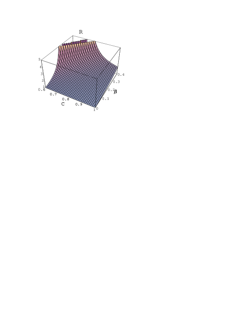
Figure 10: The dependence of the ratio, $R$, (see Eq. 20) of the normalized variability amplitude in the X-ray and in the $UV$ band on $\beta_{d}$ and $C$. Other parameters: $a=0.5$, $A=4$.

3.2.3 Application of the toy model to monitored objects

A few AGN were recently monitored both in the UV and X-ray bands, and the results of these campaigns can be used directly to determine the properties of the cloud distribution in those sources within the frame of our random variability picture.

Observational data provides us either directly with the rms values both in UV and X-rays or with the value of variability factor $\cal A$ in those bands. Data were taken from Goad et al. (1999) and Edelson & Nandra (1999) for NGC 3516, from Nandra et al. (1998) for NGC 7469, from Edelson et al. (1996) for NGC 4151 and from Clavel et al. (1992) for NGC 5548.

Observational estimation of the ratio of the X-ray to UV luminosity is unfortunately rather complex. Most sources have red optical/UV spectra, with negative slopes on a $\nu F_{\nu}$ plot. It most probably means that the objects are considerably reddened, with a significant fraction of the energy reemitted in the IR (e.g. Wilkes et al. 1999). A conservative discussion of this problem for NGC 4151 by Edelson et al. (1996) concluded that X-ray luminosity is 3 times smaller than the UV/optical/IR luminosity. The situation for the other objects looks qualitatively similar. Also this ratio determined for the Gondek et al. (1996) composite is of the same order (i.e. 0.3). We therefore adopted $L_{X}/L_{UV}$ ratio equal 1/3 for all objects.

We now fix two of the toy model parameters: the Compton amplification factor $A=4$ and X-ray albedo $a=0.5$. Now, two observed quantities (normalized variability amplitudes in the UV and X-ray bands) allow us to calculate the covering factor $C$, the number of clouds, $N$, the probability of upscatering for a UV photon $\gamma$, and the contribution of the dark sides of clouds, $\beta_{d}$. The results for the four selected objects are given in Table 1.

The covering factor obtained is the same for all objects, as it is determined purely by the X-ray to UV luminosity ratio. The assumption of $L_{X}/L_{UV}=1/3$ influences the obtained value of the covering factor, but not strongly. A value of 0.5 would give $C=0.86$ and a value of 0.1 would give $C=0.96$. The last value is more appropriate for quasars than for Seyfert 1 galaxies. Also the adopted value of the albedo does not influence the results significantly: $a=0.3$ would give a covering factor of 0.86 for our objects.

The value of $\beta_{d}$ is equal to zero in two of our objects, since the normalized variability in the UV and X-rays are equal and no contribution from the dark sides is required.

Table 1: Toy model parameters for AGN.

Object	$rms_{UV}$	$rms_{X}$	C	N	$\gamma$	$\beta_{d}$
NGC	observed	observed
3516	0.333	0.357	0.90	1180	0.047	0.04
7469	0.167	0.167	0.90	5400	0.044	0.00
4151	0.009	0.024	0.90	2610	0.095	0.39
5548	0.222	0.222	0.90	3050	0.044	0.00

3.3 Mean spectrum from radiative transfer codes

Since the complete solution of radiative transfer equation within the cloud system are extremely time consuming, we used the toy model results to guide our choice of the model parameters. Now we can test our toy model parameterization against numerical results.

The present version of the radiative transfer computations does not include yet the finite size of the hot Comptonizing medium located close to the black hole, so the effect of Comptonization is replaced by a central point source emitting a power law continuum of an arbitrary slope and extension.

Figure 11: The mean spectrum (thick line) calculated with the coupled codes titan and noar for the following parameters of the shell: log$n=14$, log $N_{H}=26$, covering factor $C=0.9$. The incident primary radiation was assumed to be a power law extending from 1 eV to 100 keV, with energy index $\alpha=1$, and ionization parameter $\xi=300$. The size of the central source was neglected. The two other spectra (thin lines) show the high and low state expected as variations at a 2 standard deviation level in the case of $N=1000$ clouds (see Sect. 2.4.1).

The mean spectrum from our computation is shown in Fig. 11, along with the parameters used.

Spectral features in the UV and X-ray band are clearly visible, including iron $K_{\alpha}$ line and a number of emission lines in soft X-rays. These features are due to ’reflection’ of X-rays by partially ionized clouds.

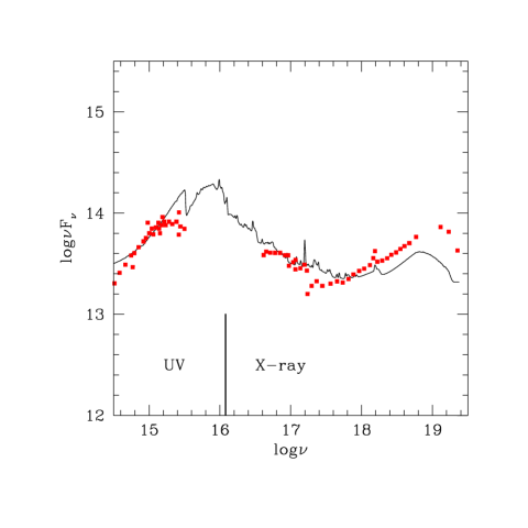
Figure 12: The mean spectrum calculated with the coupled codes titan and noar for the parameters as in Fig. 11, but with the contribution from the dark sides neglected, as required by the variability analysis of the Seyfert 1 galaxy NGC 5548 (see Table 1). Filled squares show schematically the observed spectrum of NGC 5548 after Magdziarz et al. (1998).

We can now estimate from the computations some of the toy model parameters.

The ratio of the X-ray to UV luminosity can be now calculated from the model, assuming a certain division between these two energy bands. Looking at the Fig. 11 we clearly see the two-component character of the spectrum, with a big blue bump extending roughly to 50 eV, and an X-ray component of roughly a power law shape. Therefore we adopt 50 eV as a division point between the UV and X-ray bands.

The observed $L_{X}/L_{UV}$ ratio depends on the adopted size of the central cloud. If this size is neglected, as in this computation, the $\left({L_{X}\over L_{UV}}\right)_{obs}$ is equal to 0.24. The assumption of $r_{X}/r_{UV}=0.7$ reduces it to 0.22, so the effect of this uncertainty on the spectral appearance is not essential.

The frequency-averaged albedo in the full numerical computations, calculated as a ratio of the X-ray luminosity to the total incident luminosity, is equal to 0.58, in agreement with the values used to construct Fig. 6-8.

We can also calculate the effect of leaking through the dark sides of the clouds. For the presented computations $\beta_{d}=0.26$.

This value is much higher than in three out of the four monitored objects. It means that in Seyfert galaxies like NGC 5548, the column density of clouds should be larger than $N_{H}=10^{26}$ cm^-2 adopted in the computations. Therefore we compare the mean observed spectrum of NGC 5548 with the computed one, neglecting the contribution from the dark side of clouds, i.e. $\beta_{d}=0$ (see Fig. 12). The predicted spectrum may still be too bright in far UV range, which suggests that the ionization parameter adopted in the numerical computations was slightly too low. Also, the high energy cut-off adopted in the computations (100 keV) should be increased in order to fit this particular data. When the dark side contribution is neglected, the obtained $\left({L_{X}\over L_{UV}}\right)_{obs}$ ratio is higher, equal to 0.43.

From the toy model, if we assume $C=0.9$, $a=0.58$ and $A=4$ we obtain $\left({L_{X}\over L_{UV}}\right)_{obs}=0.38$. Therefore, the toy model reproduces surprisingly well the complex solutions of the radiative transfer if supplemented with appropriate values for the X-ray albedo and dark side emission efficiency.

3.4 Random variations from the radiative transfer codes

Random rearrangement of the clouds leads to minor changes of the effective covering factor in the direction towards the observer. We illustrate here these changes using the results of the numerical computations described in detail in the previous section.

Assuming the number of clouds, $N=1000$, we show two representative examples of the observed spectra at any moment of time (see Fig. 11). Since the contribution of the dark sides was non-negligible for the adopted parameter set, the variations seen in UV are of much lower amplitude than the variations of the X-ray emission.

4 Discussion

4.1 Quasars, Seyfert 1 galaxies and Narrow Line Seyfert 1 galaxies

Various classes of AGN differ systematically although it may not necessarily mean that they form truly separate classes. Instead, they rather represent various parts of the same continuous multidimensional distribution in some parameter space. Interesting approach to this problem was formulated within the frame of the method of principal component analysis (PCA) by Boroson & Green (1992) and Brandt & Boller (1998).

Our cloud model can well reproduce the typical trends. Stronger Big Blue Bump component characteristic of quasars and narrow line Seyfert 1 galaxies (NLS1) corresponds to a larger covering factor, of order of 0.98, instead of 0.9 obtained for Seyferts (see Sect. 3.2.3). Stronger variability of NLSy1 galaxies in comparison with quasars (see Leighly 1999) means that the number of clouds in these objects is of order of $10^{4}$, not much higher than for Seyfert 1 galaxies but an order of magnitude lower than in quasars.

These trends are not surprising. If we imagine for simplicity that all accreting clouds are identical, the number of clouds present would depend on the accretion rate and the travel time of clouds scales with the mass of the black hole, $N\propto\dot{M}M$. The covering factor would be given by the number of clouds and the size of the typical radius $r_{UV}$, scaling again with the mass, i.e. $C\propto N/M^{2}\propto\dot{m}/M$. This would mean that the covering factor $C$ is mostly determined by the luminosity to the Eddington luminosity ratio and both quantities are high in quasars and NLSy1 galaxies, while additionally the number of clouds depends on the mass and accretion rate, causing fainter objects to vary more than brighter objects with the same luminosity ratio.

4.2 Relative normalized amplitudes in X-rays and UV

Our model of variability predicts that the normalized amplitude of variations in X-rays should be equal to that in the UV if the contribution of the dark sides of the clouds to the UV emission can be neglected. Therefore, equality of these two amplitudes in a number of objects is expected. In those objects which show stronger variability in the X-ray band than in the UV band, a certain level of contribution from the dark sides is required.

This kind of behavior is quite in contrast with the frequently adopted picture in which the UV variability is caused by reprocessing of the variable X-ray flux. In this case the basic effect is in the change of the temperature of the illuminated cool gas. Equality of the normalized variability amplitudes in X-rays and in the UV requires fine tuning. We can estimate the effect in the following way.

In Fig. 13 we show the result of complete thermalization of the X-ray flux varying by a factor 2, described using a simple black body approach. The variability in the UV (1315 Å) depends on the mean value of the cold matter temperature $T_{cl}$. $R(T_{cl})$ is close to 1 only for a single specific value of the mean cloud temperature ($\sim 27000$ K). For colder matter, the UV variability is stronger since we are at the exponential part of the Planck function. Hotter clouds exhibit variations with an amplitude four times smaller than the amplitude in the X-rays which caused variations.

Figure 13: The ratio $R$ (see Eq. 20) of the normalized variability amplitude at 1315 Åand 2 keV as a function of cold matter temperature within the frame of reprocessing scenario of $UV$ variability. We assumed factor 2 variability of the variable irradiating X-ray flux

Fine resolution monitoring of the Seyfert galaxy NGC 7469 in the UV and X-ray bands show that, at least in this source, the relative amplitudes in the UV and X-ray bands are the same. It is easily explained within the frame of the cloud model by adopting a relatively low contribution of the dark sides of the clouds to the UV band, i.e. rather high column density of the clouds. In the case of the simple reprocessing picture, the same value for both normalized amplitudes is difficult to obtain (see Fig. 13). The typical behavior of the other three sources considered in Sect. 3.2.3 also conforms to the cloud model expectations, with one more source showing the same amplitude ratio (NGC 5548). Unfortunately, the number of objects monitored both in the UV and X-rays is still low.

Within the frame of our model, large amplitude of variations should be unavoidably accompanied by occasional complete coverage of the X-ray source due to large statistical deviations. Such events are actually observed; the best documented case was seen in NGC4051 (Guainazzi et al. 1998, Utley et al. 1999).

Surprisingly low amplitude in the optical band, or no variations seen in some sources strongly variable in X-ray band (see Miller 1999,: also Boller, privite communication), can be also accommodated by our model as it may correspond to a very large contribution of the dark sides of clouds. However, this effect may be also due to the domination of the optical band by the starlight of the host galaxy.

Our obscuration model of variability cannot explain those events which are characterized by larger amplitude variations in the UV than in the X-ray band. Such events are occasionally observed in some sources. For example, NGC 5548 showed a spectacular brightening in the UV in 1984 which was accompanied by a very moderate brightening in X-ray band (see Clavel et al. 1992). The nature of such long timescale events should be definitively different from random variability of the covering factor discussed in this paper.

4.3 Hard X-ray slope and high energy cut-off

The prediction of the obscuration model of variability is that nothing actually changes within the source. Random rearrangements of clouds blocking our line of sight to the X-ray emitting region do not change either the optical depth, or the temperature of the hot plasma. The amount of reflection also should in principle not vary with respect to the primary emission.

Observational constraints on the variability of the slope of the X-ray ’primary’ component are not conclusive. A number of studies suggest that strong variations in the luminosity are not accompanied by spectral changes (e.g. Turner, George & Netzer 1999 for Akn 564, George et al. 1998 for NGC 3227; see also Gierliński et al. 1997 for Cyg X-1). However, Zdziarski, Lubiński & Smith (1999) and Done, Madejski & Życki (1999) suggest the presence of a correlation between the slope of the primary component, amount of reflection and the source luminosity for NGC 5548. The problem of decomposition of the spectrum into two components - primary and reflected - is difficult for the short time sequences of the data used in variability studies. Also, a fraction of the reflection comes from very large distances and does not respond to the nuclear emission within the observed time, as suggested by the remnant emission observed during the off state in NGC 4051 (Guainazzi et al. 1998)

The prediction of the model that no spectral variability in X-rays is expected is also not firm. In a real situation, if there are any temperature gradients within the hot cloud and the cold clouds are located on a range of distances with a complex overlapping pattern, we can expect some weak spectral variations caused by cloud eclipses. However, the predictions of the trends would require either an ad hoc parameterization, or a dynamical study of cloud formation and disruption which is beyond the scope of the present paper.

5 Conclusion

The cloud scenario offers an interesting quasi-spherical model of accretion onto a central massive black hole. It explains the observed large ratio of the Big Blue Bump luminosity to the X-ray luminosity. The second prediction of the model is the variable obscuration of the X-ray source. It can explain the following observed trends:

• $\clubsuit$ significant X-ray variability not accompanied by the change of the spectral slope; this is due to random cloud redistribution without changes of the covering factor,

• $\clubsuit$ amplitude of the variability in X-ray band larger or equal to amplitude in UV band: this is due to the contribution from the dark sides of clouds,

• $\clubsuit$ variability timescales ranging from $10^{2}$ s to $10^{6}$ s; this is due to the size of the optically thick clumps, the size of the X-ray medium and Keplerian motion.

Variability analysis indicates that in many objects the column density of the clouds is very large, $N_{H}>>10^{26}$cm^-2 suggesting their origin in violent disk disruptions.

Further progress is required in order to incorporate the finite size of the hot central cloud into the numerical computations of the radiative transfer, and to address the problem of intrinsic variability.

Appendix A : Energy conservation and Compton amplification factor

We denote the number of UV photons inside the radius $r_{UV}$ by $N_{UV}$, the number of X-ray photons by $N_{X}$, and their mean energies by $E_{UV}$ and $E_{X}$, correspondingly. We also introduce the efficiency $\eta_{X}$ of creating an X-ray photon of an energy $E_{X}$ during subsequent scatterings within the hot plasma and the efficiency $\eta_{UV}$ of creating UV photons from an absorbed X-ray photon of energy $E_{X}$. The value of $E_{X}$ and $\eta_{X}$ depend sensitively on the hot cloud optical depth $\tau$ and its electron temperature $T_{e}$ since they are related to the spectral shape of produced X-rays. $\eta_{UV}$ is simply given by

$$\eta_{UV}=E_{X}/E_{UV}.$$ (35)

The conservation law for the number of UV photons within the system is given by

$$(P_{esc}^{UV}+P_{ups}^{UV})N_{UV}=\eta_{UV}P_{abs}^{X}N_{X}$$ (36)

where all the probabilities are given by Eqs. (1) - (7).

The conservation law for a number of X-ray photons is given by

$$(P_{esc}^{X}+P_{abs}^{X}+P_{dark}^{UV})N_{X}=\eta_{X}P_{ups}^{UV}N_{UV}$$ (37)

Those two equations can be combined into the condition of the stationarity

$$(P_{esc}^{UV}+P_{ups}^{UV})(P_{esc}^{X}+P_{abs}^{X}+P_{dark}^{UV})=\eta_{X}\eta_{UV}P_{ups}^{UV}P_{abs}^{X}$$ (38)

If true losses from the system (i.e. leak through the dark sides and escape) are equal zero, $\eta_{UV}\eta_{X}$ must be equal 1, i.e. no Compton amplification is possible (or required) and the hot and cold plasma achieve thermal equilibrium. Only stationary losses and energy supply to the hot plasma support the existence of the two strongly different media.

The product $\eta_{UV}\eta_{X}$ is directly related to the Compton amplification factor $A$ of the hot plasma

$$\eta_{UV}\eta_{X}=A(\tau,T_{E})$$ (39)

Substituting this relation into Eq. 38 we obtain the stationarity condition 9.

We can also determine the ratio of the bolometric luminosity in X- ray and UV spectral components.

$$\left({L_{X}\over L_{UV}}\right)_{int}={N_{X}E_{X}\over N_{UV}E_{UV}}.$$ (40)

The $N_{X}/N_{UV}$ ratio can be determined from Eq. 36

$$\left({L_{X}\over L_{UV}}\right)_{int}={(P_{esc}^{UV}+P_{ups}^{UV})\over P_{abs}^{X}(1-\beta_{d})}{E_{X}\over E_{UV}\eta_{UV}}$$ (41)

where the last term is equal 1 on the basis of Eq. 35.

Appendix B : Mean number of clouds on the line of sight

We assume that $N$ clouds of radius $r_{cl}$ are homogeneously distributed in a shell of radius $r_{UV}$ whose thickness is small with respect to its radius. The coverage factor of the system of clouds is $\Omega/4\pi=C$. The mean number of clouds on the line of sight, $N_{ls}$, is given by:

$$N_{ls}\sim N{X\over 4C}$$ (42)

where $X=(r_{cl}/R)^{2}$.

The total number of clouds is related to the coverage factor by:

$$X=1\ -\ (1\ -\ C)^{1/N}$$ (43)

This expression can be expanded to the first order:

$$X={1\over N}Ln{1\over 1-C},$$ (44)

provided that $Ln{1\over 1-C}\ll N$. This is easily achieved except for extremely small values of $1-C$ (in our case $1-C\sim 0.1$). One deduces thus that $X\sim 2/N$, and therefore $N_{ls}\sim 1/C$.