Strong and weak lensing analysis of cluster Abell 2219 based on optical and near infrared data

Abstract

We present a gravitational lensing study of the massive galaxy cluster A2219 (redshift 0.22). This investigation is based on multicolour images from U through H, which allows photometric redshifts to be estimated for the background sources. The redshifts provide useful extra information for the lensing models: we show how they can be used to identify a new multiple-image system (and rule out an old one), how this information can be used to anchor the mass model for the cluster, and how the redshifts can be used to construct optimal samples of background galaxies for a weak lensing analysis. Combining all results, we obtain the mass distribution in this cluster from the inner, strong lensing region, out to a radius of 1.5$h_{50}^{-1}Mpc$. The mass profile is consistent with a singular isothermal model over this radius range.

Parametric and non-parametric reconstructions of the mass distribution in the cluster are compared. The main features (elongation, sub-clumps, radial mass profile) are in good agreement.

1 Introduction

Gravitational lensing is a very powerful phenomenon for determining the mass distribution in clusters of galaxies at various scales. In the inner parts of clusters, giant arcs and multiple image systems give immediate constraints on the cluster core radius and velocity dispersion. Usual values are between 50$h_{50}^{-1}\,kpc$ and $100h_{50}^{-1}\,kpc$ for the core radius while velocity dispersion ranges from 800$km\,s^{-1}$ to 1300$km\,s^{-1}$ (Fort and Mellier 1994). The presence of several multiple image systems at different redshifts also allows the slope of the mass distribution with radius to be probed. Such systems are more easily discovered with multicolour imaging, including IR, which lead to photometric estimates of their redshifts, as shown by Pelló et al. (1999a) for two objects at $z=4.05$ in A2390. Most cluster lens models show bimodality or elongated structures which are also found in the X-ray emission in many examples (A370, A2218, A2390, A2104).

In the outer parts, the weak distortions of background galaxies, at a few percent level, provide a direct mapping of the mass distribution on large scales (as reviewed by Mellier 1999). The general shape of the potential is then accessible as well as substructures or extensions (RXJ1716+67, Clowe et al. 1998, Hoekstra et al. 2000).

HST images are important for shear measurement thanks to the absence of a large circularization by seeing. On the other hand, the small field of view of WFPC2 limits the study to the central parts of the clusters though in a few cases mosaics of HST images have been analysed (Hoekstra et al. 1998, Hoekstra et al. 2000). Because of their angular size, ground based wide field imaging are better adapted for low redshift clusters. Mass distributions derived from weak lensing show a mass to light ratio of several hundred (see the compilation by Mellier, 1999). Comparison of X-ray and mass maps can mostly be done for low redshift clusters and it appears that the mass distribution infered from weak lensing often peaks at the same location as the X-ray emission (A2218, A370, MS1224+20, MS0302+17). At high redshift, RXJ1716+67 also shows this agreement. At the same time, orientations are quite similar which means that on large scale the gas traces the mass well.

In this paper we present a combined analysis of gravitational lensing by the cluster Abell 2219 and the properties of the lensed sources. We utilise both strong and weak lensing constraints in order to determine the mass distribution on various scales. A key component of our analysis is the use of multicolour optical and near-infrared data which is used to provide additional constraints on the redshift distribution of lensed sources.

A2219 is a rich cluster at $z=0.225$ (Allen et al. 1992) and is one of the brightest X-ray clusters detected by the ROSAT All Sky Survey. Observed also by ROSAT HRI (13.4 ks, Smail et al. 1995) and ASCA (34 ks, Cagnoni et al. 1998), A2219 has a luminosity of $L_{X}(0.1-2.4keV)=1.8\times 10^{45}erg\,s^{-1}$ (Smail et al. 1995) and $L_{X}(2-10keV)=3.8\times 10^{45}erg\,s^{-1}$ corresponding to a temperature $T_{X}=9.5keV$ (Allen 1998). Smail et al. (1995) show the HRI map to be in a agreement with the general elongated shape of the cluster on large scale but a misalignement is present on smaller scales (X-ray emission in A2218, Kneib et al. 1995, doesn’t follow the light either in the very center). The mass derived from lensing happens to be two times higher than the X-ray mass according to Allen (1998), though assuming a spherical mass distribution. Infrared data at 15$\mu m$ obtained by Barvainis et al. (1999) with ISO show 5 sources. The 20cm VLA survey of Abell clusters detected three sources of which the brightest has a flux of 212 mJy (Owen et al. 1992). These sources are identified as RG1, RG2 and G2 on figure 1. Their spectroscopic follow up identified RG1 as a radio galaxy at $z=0.2070$ (Owen et al. 1995). Other observations have been done at 28.5 Ghz (Cooray et al. 1998) and 408 Mhz (Ficarra et al. 1985) for which the peak of emission coincides with galaxy RG1.

Figure 1: Composite B and I image of cluster A2219. The objects labels are on the right hand side. North is right and east is up.

A plan of the paper follows. In section 2 we present the multiband observations obtained for this work as well as already published images. Section 3 is devoted to the determination of photometric redshifts using 5 filters from $U$ to $H$. Then, the cluster mass distribution in the central part is modeled using mainly two systems of multiple images in Section 4. The weak distortions of background galaxies are studied in the next section with a comparison of the mass profiles coming from these various methods.

2 Observations

Observations of cluster A2219 have been conducted at the 4.2m William Herschell Telescope at La Palma, Spain. Images in $B$ and $I$ band were acquired at prime focus in may 1998 in excellent conditions with a seeing of 0.8  in $B$ and in $I$. Exposure time is 2400s in $B$ and 3600s in $I$. In each filter, two pointings of the 2K$\times$4K camera resulted in a wide field of 16$\times$15  with 0.237/pixel centered on the cluster.

The infrared observations were made over three nights in June 1998 at WHT in june 1998 with the Cambridge Infra Red Survey Instrument (CIRSI). The individual exposures were either 30 or 60 seconds long, and totalled 2.48 hours. CIRSI is made of four 1k$\times$1k chips with 0.32/pixel. After shifting and adding the images, the useful field of view in the cluster center is 4.8$\times$4.8.

In order to cover a wavelength range as broad as possible, we use also the $U$ image obtained by Smail et al. (1995) at the 5m Hale telescope at Palomar. Finally, their $V$ image taken at Keck complements this multicolour description of cluster A2219.

Flux calibration was made with standard stars in M92 (WHT Prime Focus user manual) and from Landolt (1992). Image reduction was performed using IRAF packages. The $1\sigma$ limiting surface brightness for each image is, in $mag/\arcsec^{2}$: $U=26.3$, $B=27.2$, $V=27.3$, $I=25.9$ and $H=23.6$.

3 Photometric estimates of the redshifts

The acquisition of images in five filters from $U$ to $H$ enables us to derive photometric redshifts for the inner part of cluster A2219. Object detection is performed in the $I$ band with the SExtractor package (Bertin and Arnouts 1996) with the requirements of a minimal area of 5 pixels and a detection threshold of 1.5 $\sigma$. The resulting catalog contains 1427 objects in a 4.8$\times$4.8square.

Photometric redshifts are computed using the code hyperz (Pelló et al. 1999b, Bolzonella et al. 2000 in preparation) with the following prescriptions:

– four star formation histories are adopted: an instantanneous burst, exponentially decreasing star formation rates with characteristic times scales of 1 Gyr and 5 Gyr, and a constant star formation.

– four metallicty abundances are considered: $Z_{\odot}/50,Z_{\odot}/5,Z_{\odot}$ and $5Z_{\odot}$.

– internal extinction was allowed to vary in the range $A_{V}=0$ to 1.2 mag.

3.1 Redshift distribution of the whole sample

The global redshift distribution of galaxies in the cluster center is displayed in figure 2. The peak of the distribution appears at $z=0.35$ which compares well with the cluster redshift ($z=0.225$, difference of $\simeq 0.1$ in redshift). The second peak around z=1 may be an artefact caused by the absence of any $R$ image. The 4000Å discontinuity redshifted at $z=1$ lies between the $V$ and $I$ filters hence $R$ band photometry would locate the objects redshift with a much better accuracy when the 4000Å break lies in this wavelength range. Photometric redshifts higher than 3 still require individual inspection as most of them correspond to faint objects which are only detected in the $I$ or $V$ band (figure 5).

Figure 2: Photometric redshift distribution in the field of A2219 derived with filters $UBVIH$.

The reliability of these photometric redshifts can be estimated through simulated catalogs. 2000 galaxies were simulated with magnitudes in $U,B,V,I,H$ and randomly distributed from $z=0$ to $z=6$, with the same metallicities, star formation rates and absorption as before. Figure 3 shows their photometric redshifts derived by the Pelló et al. code versus the input model redshifts. Some anomalies in Figure 2 can be explained via these simulations. It appears that the secondary peak in the redshift distribution at $z\simeq 1$ may be an artifact caused by the degeneracy in the method and the cluster peak appears shifted to a slightly higher redshift for a similar reason. No great significance should be attached to sources with $z>3$. The simulation was considering a typical photometric error of 0.1 mag. while the objects with $z_{phot}>3$ in A2219 have much higher uncertainties which can reach 0.5 or 1 mag.

The best illustration of the importance of an $H$ band image is given by comparison of the simulations in figures 3 and 4. The first one, computed using information in the IR, shows a much better correspondance between the model and the photometric redshifts than the second one which doesn’t make use of any measurement in the IR. In particular, the redshift determination around $z\simeq 2.5$ is worse without data in $H$ as the 4000Å break should lie between $I$ and the missing $H$.

Figure 3: Photometric redshift versus model redshift for 2000 galaxies using simulated data in $U,B,V,I,$ and $H$.

Figure 4: Photometric redshift versus model redshift for 2000 galaxies using simulated data in $U,B,V$ and $I$.

Figure 5: I - $z_{phot}$ relation for the 1427 objects detected in $I$ in the central part of the cluster.

3.2 Individual cases: the triple arc and a new high redshift multiple system

The technique of using multicolour data to identify multiple images systems in clusters lenses has been demonstrated as a very powerful technique by Pelló et al. (1999a). Two such examples at $z=4.05$ in cluster A2390 have been studied in details, giving some clues on their stellar content.

In A2219, Smail et al. (1995) mentioned a very blue giant arc (object L) consisting of three images. All three images have the same colour and none of them is detected in the $H$ band. The arc SED reveals a quickly rising spectrum towards the UV (figure 6). However, the redshift is poorly constrained by photometric data as no strong discontinuity is enclosed by any filters. The acceptable domain in the parameter space (redshift, age) is highly degenerate extending from $z=0$ to $z=2.6$ with an age between 0.02Gyr and 2.5 Gyr (figure 7).

Figure 6: Spectral energy distribution of the triple arc L. The point in $H$ is an upper limit. The solid line corresponds to a 0.09 Gyr burst of star formation with solar metallicity at $z=1.5$. Wavelength in rest frame (Å) is given at the top.

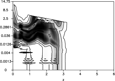
Figure 7: Probability map for the solutions in (redshift, age) for the triple arc L. The solid lines are the contours at 68%, 95% and 99% confidence level. Age is given in Gyr.

A second multiple image system seems to be present in A2219 at much higher redshift. Three red objects appear in the cluster center, namely objects A, B and C in figure 1. Objects A and B show very similar SEDs, undetected in $U$ and very faint in $B$ and $H$. Object C is even fainter but contaminated by a neighbouring blue object. A good solution for object A appears at $z=3.6\pm 0.4$ with an age ranging from 0.01Gyr to 1Gyr (figure 8). Object B is in good agreement with this result in spite of contamination by the cD red enveloppe, and object C to a lesser extent since its magnitude measurement is more uncertain due to its faintness and possible contamination in the case of the $B$ image. Another solution at low redshift appears to be possible but with a much smaller significance as the expected IR flux should be much higher than what is observed. Moreover, the elongated shape and the position angle of A are consistent with what is expected for a lensed object and B shows no distortion which is also understandable as it lies in an area with a smaller shear. Hence, we adopt a photometric redshift of $3.6\pm 0.4$ for A and B (figure 9).

Table 1: Photometry of lensed objects in A2219 according to the numbering by Smail et al. (1995). Coordinates are given with respect to the central cD. Object C is located close to a blue object and object B is probably contaminated by the red cD enveloppe.

Object	X (′′)	Y (′′)	$U-B$	$\sigma_{U-B}$	$B$	$\sigma_{B}$	$B-V$	$\sigma_{B-V}$	$B-I$	$\sigma_{B-I}$	$B-H$	$\sigma_{B-H}$
A	12.9	29.6	-	-	27.00	0.33	1.74	0.45	3.16	0.35	4.02	0.39
B	-10.4	23.4	-	-	27.41	0.80	2.15	0.87	3.48	0.84	4.48	1.28
C	-32.5	-8.3	-	-	27.07	0.25	0.82	0.39	2.39	0.32	-	-
N1+2	-13.7	10.7	-0.77	0.13	22.65	0.08	0.65	0.15	1.82	0.11	3.08	0.30
N3	14.6	21.0	-0.52	0.22	23.49	0.14	0.49	0.23	2.18	0.19	3.99	0.27
L3	-3.6	-26.5	-0.73	0.13	23.31	0.05	0.20	0.09	0.83	0.11	-	-

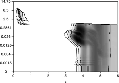
Figure 8: Probability map for the solutions in (redshift, age) for object A. The solid lines are the contours at 68%, 95% and 99% confidence level. Age is given in Gyr.

Figure 9: Spectral energy distribution of object A. The point in $U$ is an upper limit. The solid line corresponds to a burst of star formation seen at an age of 0.03Gyr with 5$Z_{\odot}$ at $z=3.6$.

4 Mass modeling of the inner part of the cluster

A2219 is a luminous X ray cluster, one of the brightest clusters seen in the ROSAT All Sky Survey (Allen at al. 1992). The general shape of its X-ray emission obtained with ROSAT HRI shows an elliptical morphology aligned with the axis defined by the two brightest galaxies with a luminosity of $L_{X}=1.8\times 10^{45}$ erg s${}^{-}1$. (Smail et al. 1995). A first mass model was derived by these authors based on two multiple image systems: the triple arc L and objects $N_{1+2}$ - $N_{3}$. However, it seems that N₃ is not likely to be a counter image of N₁₊₂ as their colour indices $B-I$ and $B-H$ are clearly different (table 1). Moreover, the redshifts of objects $N_{1+2}$ and $N_{3}$ are poorly constrained by their photometry. Hence, we have only used the two systems already described, the arc L and the faint red objects A and B. Investigation of the mass distribution in the cluster center was made in two independent ways following methods developed by Kneib et al. (1996) and AbdelSalam et al. (1998a).

4.1 Cluster mass distribution as a superposition of a cluster and a galaxy components

The Lenstool facility developed by J.P. Kneib allows us to consider the cluster mass distribution of A2219 as the superposition of potentials centered on the two brightest galaxies and potentials on all galaxies brighter than $I=19$. All potentials follow a truncated pseudo isothermal elliptical mass distribution (Kassiola and Kovner 1993).

Following Kneib et al. (1996), for each galaxy halo, the velocity dispersion $\sigma_{0}$, the truncation radius $r_{t}$ and the core radius $r_{0}$ are scaled to the galaxy luminosity computed from the observed $I$ magnitude. The scaling relations used for the galaxy halos are:

$$\sigma_{0}=\sigma_{0\ast}\left({L\over L_{\ast}}\right)^{{0.25}},$$ (1)

$$r_{t}=r_{t\ast}\left({L\over L_{\ast}}\right)^{{0.5}},$$ (2)

$$r_{0}=r_{0\ast}\left({L\over L_{\ast}}\right)^{{0.5}}.$$ (3)

The scaling relations adopted are motivated by the properties of the Faber Jackson relation.

The orientation and ellipticity of the galaxy halos are taken from the observed values of the light distribution while $\sigma_{0\ast}$ corresponds to a mass to light ratio of 10 in $I$. $r_{0\ast}$ and $r_{t\ast}$ are fixed at 0.15 and 20 $h_{50}^{-1}\,kpc$.

The cluster components are modeled by two large scale mass distributions centered on the two brightest galaxies. Their orientations, ellipticities, velocity dispersions, core radius and truncation radius are left as free parameters.

The optimisation was made using the constraint that objects A and B are two images of the same source at $z=3.6$ and that arc L is a triple arc. The resulting value for the arc redshift is $z_{L}\simeq 1.5$ which lies inside the large allowed range derived by the photometric analysis. A third image for the $z=3.6$ system is predicted to be at $x=-36$and $y=-3$, 6  away from object C. The cluster mass distribution is shown in figure 10. The main clump has a velocity dispersion of 1120 $km\,s^{-1}$ and the second one has 540$km\,s^{-1}$. The cluster mass inside a radius of 150 $h_{50}^{-1}\,kpc$ is 1.2 10${}^{14}M_{\odot}$, similar to AC114 (Natarajan et al. 1998), and $M=3.4\,10^{14}\,M_{\odot}$ inside 300$h_{50}^{-1}\,kpc$, which is 30% smaller than in A370 (Bézecourt et al. 1999).

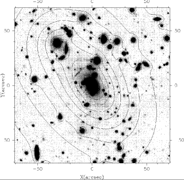
Figure 10: Mass distribution in A2219 represented by a cluster component plus a galaxy component overlayed on the $I$ band image.

4.2 Non-parametric mass reconstruction

The non-parametric reconstruction method works with a pixellated mass distribution in the lens plane, say $N\times N$ pixels with inter-pixel spacing $r$. Consider the $mn$-th pixel is a Gaussian circle with dispersion $r/2$ and peak height $\kappa_{mn}$ in units of the critical surface mass density. For a background source at an unlensed position $\beta$, the appropriately scaled time-delay in the direction $\theta$ is

$$\tau(\mbox{\boldmath$\theta$})=\frac{1}{2}(\mbox{\boldmath$\theta$}-\mbox{\boldmath$\beta$})^{2}-\frac{D_{ds}}{D_{s}}\sum_{mn}\kappa_{mn}\psi_{mn}(\mbox{\boldmath$\theta$}),$$ (4)

where

$$\psi_{mn}(\mbox{\boldmath$\theta$})=\frac{1}{\pi}\int_{mn}e^{\frac{-2\xi^{2}}{r^{2}}}\ln|\xi|d^{2}\theta^{\prime},$$ (5)

where $\xi=\mbox{\boldmath$\theta$}^{\prime}-\mbox{\boldmath$\theta$}_{mn}$. The quantity $\psi_{mn}$ is the coefficient of the deflection potential at $\theta$ due to the $mn$-th pixel only. Thus the contribution of the $mn$-th pixel to the lens potential is $\kappa_{mn}\psi_{mn}$ (AbdelSalam et al. 1998a).

Lensing observations in clusters of galaxies are:
$\bullet$ Positions of multiple images on the sky, i.e $\nabla\tau(\mbox{\boldmath$\theta$})=0$.
$\bullet$ Orientations and elongation of individual faint distorted objects, for example magnification in direction $\theta_{x}^{\prime}$ is at least $\delta$ times that along perpendicular direction $\theta_{y}^{\prime}$, then

$$\delta|\frac{\partial^{2}}{\partial\theta_{x^{\prime}}^{2}}\tau(\mbox{\boldmath$\theta$})|\leq|\frac{\partial^{2}}{\partial\theta_{y^{\prime}}^{2}}\tau(\mbox{\boldmath$\theta$})|.$$ (6)

Both observations provide us with linear constraint equations on the unknowns $\beta$ and $\kappa_{mn}$. Using constraints from both above observations combines the strong and weak lensing regimes simultaneously and breaks the mass-sheet degeneracy upon using at least two different source redshifts (AbdelSalam et al 1998b).

Mass maps are then reconstructed by use of quadratic programming to minimize $M/L$ variations while satisfying the lensing constraints exactly. So we minimize

$$\sum_{mn}\left[\kappa_{mn}-L_{mn}\sum_{i^{\prime}j^{\prime}}\kappa_{i^{\prime}j^{\prime}}\right]^{2}+\epsilon^{4}\sum_{mn}(\nabla^{2}\kappa_{mn})^{2},$$ (7)

where $L_{mn}$ is the light distribution of the cluster and $\epsilon$ is a smoothing parameter.

The mass distribution was determined according to the same constraints as before plus the orientation and ellipticity of the faint distorted objects ($\sim$ 20 points on a grid inside the $143\arcsec$ field excluding the strong lensing region). We assumed a redshift of 1 for these objects. In the modelling, two main clumps appear centered on the two brightest galaxies with offsets of about 2.5   for G1 towards the direction of G2 and about 6  for G2 towards G1. As a smoothing by a Gaussian with $\sigma=3.39\arcsec$ was applied, the mass peaks coincides well with the light peaks. Moreover, an extension of the mass distribution towards the upper right of the cD agrees well with the presence of several galaxies in this part of the cluster.

On reconstructing the multiple image system at $z=3.6$ given only constraints from objects A and B, we find that they are the outcome of a seven-image system configuration. The image C (which was not included in the input constraints) is predicted exactly as where it is in the cluster (see figure 1). For the four remaining images, two lie in the cD and two are located in empty places.

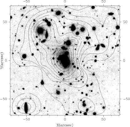
Figure 11: Mass distribution in A2219 derived by AbdelSalam et al. (1998a) method. The shear field measured in section 5 is indicated.

The mass profiles from both methods (Kneib and AbdelSalam et al.) for the cluster center agree well within 25% at the location of the multiple image systems (figure 18) and increase at the same rate with radius. The ratio of the main clump, centered on the cD and within 20, to the second one, centered on galaxy G2 and within 20, is 1.32 and 1.39 according to the first and second method respectively which show an excellent agreement. Both models require a bimodal mass distribution with a possible extension to the north west. The triple arc is well reproduced by the models, as well as objects A and B but object C or possible additional images remain to be investigated.

5 Weak lensing analysis

At large radii from the cluster centre, the distortion in the shapes of the background galaxies is small. This is the regime of weak gravitational lensing. The lensing signal is obtained statistically, by averaging the shapes of many background sources. However, the observed shapes cannot be used directly, as various observational effects, like PSF anisotropy and seeing, have changed the images of the galaxies.

To measure the weak distortion we follow the procedure described in Kaiser et al. (1995), Luppino & Kaiser (1997), and Hoekstra et al. (1998).

5.1 Objects catalogs

The first step in the analysis is to detect the images of the faint galaxies. Object detection was done in each individual image in $B$ and $I$ with the imcat software (Kaiser et al. 1995), requiring a significance higher than $4\sigma$ over the local sky background. The detected objects are not required to have a photometric redshift estimated.

We use images that were formed by combining the individual exposures by straight averaging (this avoids corrupting the PSF). Therefore cosmic rays are still present in the images. In the object catalogs we identify very significant objects, but smaller than 2 pixels, as cosmic rays. These are removed from the object catalogs.

Then the objects are analyzed, and sizes, magnitudes, and shape parameters are estimated. We remove objects for which the analysis failed. From both the $B$ and $I$ images this results in a catalog of 13207 objects, of which 5071 are detected in both the $B$ and $I$ band. Restricting the sample to objects lying outside the cluster elliptical sequence (defined by $2.4<B-I<3.2$) amounts to 11999 and 3863 objects respectively. Star-galaxy separation was done by plotting the apparent magnitude versus half-light radius. This allows us to select moderately bright stars to study the PSF anisotropy. At faint magnitudes stars and galaxies cannot be separated, but at these levels the galaxies dominate the counts.

5.2 Shape measurements and corrections

Objects shapes are characterized by the polarization with its two components $e_{1}$ and $e_{2}$. The polarization is a combination of the second moments $I_{ij}$:

$$e_{1}={I_{11}-I_{22}\over I_{11}+I_{22}}$$

$$e_{2}={2I_{12}\over I_{11}+I_{22}}$$

where $I_{ij}=\int W(\theta)\theta_{i}\theta_{j}f(\theta)d^{2}\theta$, $f(\theta)$ is the surface brightness and $W(\theta)$ is a Gaussian weight function.

In order to recover the true galaxy shapes, they have to be corrected for various observational effects. PSF anisotropy introduces a systematic distortion in the shapes of the images of the faint galaxies, mimicing a lensing signal. We select a sample of moderately bright stars and quantify the PSF anisotropy as described in Hoekstra et al. (1998). Figure 12 shows the observed PSF anisotropy as a function of position on the chip for both the $B$ band (left) and $I$ band (right). The sticks indicate the direction of the major axis, and the length corresponds to the amplitude of the anisotropy. Following the scheme described in Kaiser et al. (1995), and Hoekstra et al. (1998) we are able to correct the polarizations of the faint galaxies for PSF anisotropy.

After correction for PSF anisotropy, one still needs to correct for the fact that seeing and the instrumental PSF (now isotropic) circularize the images. We follow Luppino & Kaiser (1997) and Hoekstra et al. (1998) to estimate the ’pre-seeing’ shear polarizability (Luppino & Kaiser 1997). The resulting correction depends on both the size and the magnitude of the galaxies, where the correction is largest for the smallest objects.

Figure 12: Polarization of stars in $B$ (left) and I(right) in the field of A2219.

5.3 Weak distortion

The distortion $g$ is related to the shear $\gamma$ and the convergence $\kappa$ via $g=\gamma/(1-\kappa)$. The weak lensing distortions are small compared to the intrinsic ellipticities of the sources. Thus we average the shapes of a large number of galaxies. We weight the contribution from each object using the uncertainty in the distortion, which includes both the contribution of the intrinsic ellipticities of the galaxies and the shot noise (Hoekstra, Franx & Kuijken 2000).

Selecting objects according to their magnitude reveals a higher distortion for faint objects with respect to the bright ones (figure 13). All objects detected in B or I with colour $B-I$ outside the cluster elliptical sequence are considered here, which corresponds to a number density of 50 objects per square arcmin. When all objects besides cluster members are considered, a higher signal is detected in the $B$ image than in the $I$ image probably because of a remaining contamination by cluster members in $I$ (figure 14). When restricting the sample to objects detected in both B and I and excluding the cluster members, the weak distortions are clearly detected out to 2 $h^{-1}_{50}Mpc$ away from the cluster center (figure 15). A singular isothermal sphere fit accounts for the data with a velocity dispersion of $1075\pm 100\,km\,s^{-1}$.

The derived velocity dispersion clearly depends sensitively on the assumed redshift distribution of the sources. In the above estimates we adopted the photometric $N(z)$ derived in the central field for this purpose (Figure 2). However, this could be uncertain for a variety of reasons. First, photometric redshifts cannot be derived or are poorly constrained for very faint objects as the photometry reliability decreases quickly while weak shear increases with magnitude (figure 13 for the bright and faint samples). Second, because of gravitational lensing magnification, the redshift distribution of background objects should contain more high-$z$ objects in the center than in the outside region of the cluster and photometric redshifts can only be determined in the central field. Third, the width of the cluster peak around $z=0.225$ (figure 2) appears to be very broad. This means that many cluster members appear at $z_{phot}=0.3-0.4$ which bias the $N(z)$ towards low redshifts. In this analysis all objects with $z_{phot}>3$ were removed as their redshift identification is still uncertain.

A major advance offered by the availability of multiband optical and near-IR data is that we can select objects in different photometric redshift intervals to verify the robustness of the derived mass. We have done this in such a way so as to maintain a reasonably-sized sample.

Selecting objects according to their photometric redshift shows a higher distortion when one goes to high $z$ as expected (figure 16 a, b, and c). The number of objects involved is: 330 at $z_{phot}<0.4$, 291 at $0.4<z_{phot}<0.85$ and 279 at $0.85<z_{phot}<3$. No significant signal is found in the first bin (a) as expected for cluster and foreground galaxies. The signal is marginal when the sources are selected between $z=0.4$ and $z=0.85$ (b) and becomes obvious in the highest redshift bin $0.85<z<3$ (c). This is a good verification of the reliability of photometric redshifts for weak lensing.

In order to check whether the signal detected in each redshift bin is consistent with the expected one given the velocity dispersion and redshift distribution adopted previously, a fit of the distortion profiles in the redshift bins [0.4,0.7], [0.7,1.0] and [1.0,3] has been performed assuming a SIS for the lens (figure 17). The velocity dispersion found in the last two bins is in good agreement with the value derived with the whole sample in figure 15 ($\sigma=1075\pm 100km\,s^{-1}$). The lower velocity dispersion found in the first redshift interval comes from the determination of photometric redshifts which cannot lead to a cluster peak at $z=0.225$ as narrow as what a spectroscopic survey would give. The peak in figure 2 is much broader than what it really is and many cluster members appear at higher redshifts and, as a result, the signal at $z<0.7$ is contaminated by these unlensed objects. This leads to a smaller amplitude of the distortion profile and, hence, to a lower velocity dispersion. On the contrary, the redshift bins [0.7,1.0] and [1.0,3] give coherent values which means that most of the signal detected in the global sample (figure 15) comes from this redshift range.

Another way of investigating the mass distribution is given by the magnification bias and Gray et al. (2000) have measured the gravitational depletion of number counts in the infrared for A2219. After fitting the depletion curve by a singular isothermal sphere, they derived a slightly lower value for the velocity dispersion, $\sigma=842^{+99}_{-84}km.s^{-1}$ assuming that the sources lie at $z\simeq 1$.

Figure 13: Distortion $g_{T}$ for the bright, faint, blue and red objects.

Figure 14: Distortion $g_{T}$ and SIS fit for objects detected in the B image ($\sigma=1225\,\pm 100\,km\,s^{-1}$) and in the I image ($\sigma=975\pm 125\,km\,s^{-1}$), excluding cluster members.

Figure 15: Distortion $g_{T}$ for objects detected in the B image and/or I image, excluding cluster members. The solid line is a SIS fit to the data ($\sigma=1075km\,s^{-1}$) using the redshift distribution of figure 2 for the background population.

Figure 16: Distortion $g_{T}$ for objects selected according to three different photometric redshift intervals: $z_{phot}<0.4$ (a), $0.4<z_{phot}<0.85$ (b), $0.85<z_{phot}<3$ (c).

Figure 17: Velocity dispersion of the lens derived in three redshift intervals by fitting the observed distortion profile with a SIS. The value derived with the whole sample ($\sigma=1075\,\pm 100km\,s^{-1}$, figure 15) is shown as a solid horizontal line

5.4 Mass estimates

The observed distortion $g_{T}$ is related to the dimensionless surface mass density $\kappa$, also called convergence, via the parameter $\zeta$:

$$\zeta(r,r_{max})={2\over 1-(r/r_{max})^{2}}\int_{r}^{r_{max}}g_{T}(r)d\,ln(r)$$

and also

$$\zeta(r,r_{max})=\overline{\kappa_{1}}(r)-\overline{\kappa_{2}}(r,r_{max})$$

where $\kappa_{1}(r)$ is the average $\kappa$ inside radius $r$ and $\kappa_{2}(r,r_{max})$ is the average $\kappa$ between radius $r$ and $r_{max}$.

Then, a lower limit to the mass inside radius $r$ is given by

$$M_{lim}=\pi r^{2}\zeta(r)\Sigma_{c}$$

where $\Sigma_{c}={c^{2}\over 4\pi G}<{D_{s}\over D_{l}D_{ls}}>$.

The photometric redshift distribution is used here to estimate $\Sigma_{c}$. The resulting lower limit on the radial mass profile is displayed in figure 18.

The fit of the distortion profile by a singular isothermal sphere (figure 15) is in good agreement with the mass profiles coming from the two strong lensing models, at least in the inner 45. Moreover, these two mass models lie satisfactorily above the lower limits derived by the $\zeta$ profile. As $\Sigma_{c}$ is very sensitive to the sources redshift distribution, the SIS profile would be lower by 20% if the redshift distribution of Fernandez Soto et al. (1999) is used instead of the N(z) from figure 2 ($\sigma=950km\,s^{-1}$ instead of 1075$km\,s^{-1}$). This distribution was determined in the HDF-N based on photometric redshifts and is restricted here to $B<26$. According to the SIS fit, the mass inside a radius of 300$h_{50}^{-1}\,kpc$ is $2.5\,10^{14}\,M_{\odot}$ ($4.8\,10^{14}\,M_{\odot}$ for A370, Bézecourt et al. 1999) and $4.2\,10^{14}\,M_{\odot}$ inside 500$h_{50}^{-1}kpc$ ($4.0\,10^{14}\,M_{\odot}$ in AC114, Natarajan et al. 1998).

The SIS fit provides also an estimate of the mass to light ratio inside 1$h_{50}^{-1}\,Mpc$: $M/L=210h_{50}$ in the $B$ band using total magnitudes given by Sextractor. Cluster galaxies are selected according to their $B-I$ and the resulting counts per magnitude are fitted by a Schechter luminosity function with parameters $\alpha=-0.9$ and $M_{\star}=-20.2$.

The mass map producing the observed shear field is displayed in figure 19 exhibiting a peak coinciding with the central cD. Two extensions are also visible: one towards galaxy G2 and another one which corresponds fairly well with a group of galaxies 45away to the north east of the cD. Hence, the three mass maps obtained using strong and weak lensing constraints agree very well with each other. This elongated structure follows also the X-ray emission shown in Smail et al. (1995).

The mass models in the strong and weak regime are based on different methods and their combination indicates that the slope of $M(<r)$ is smaller in the cluster periphery than in the center (figure 18). Comparison of both types of models in CL1358+62 (Hoekstra et al. 1998) showed that the weak lensing analysis underestimates the mass in the cluster center with respect to the mass derived with the constraint given by the arc at $z=4.92$ (Franx et al. 1997). A weak lensing analysis of A2218 gives a similar underestimate of the central mass (Squires et al. 1996) while we get comparable values at the location of the two multiple image systems.

Figure 18: Radial mass profile of the cluster in solar masses. Short dashed line: mass model derived with strong lensing constraints following Kneib’s algorithm, dotted line: mass model derived with AbdelSalam et al. method, solid line: mass profile corresponding to a singular isothermal sphere with a velocity dispersion of 1075$km\,s^{-1}$. Filled dots with error bars correspond to the lower limit on the mass profile derived from the distortion $\zeta(r)$. The three vertical lines give the distance of the giant arc and objects A and B with respect to the central cD. 100=458$h_{50}^{-1}\,kpc$ at $z=0.225$.

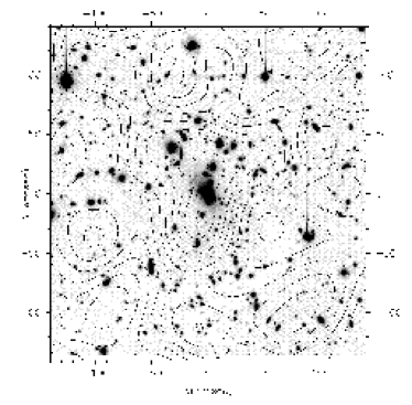
Figure 19: Mass map derived from weak lensing overlayed on a $I$ band image of A2219.

6 Conclusions

We have presented a multicolor, wide field imaging study of A2219 and studied the lensing properties of the cluster with it. A new feature of this analysis is the combination of optically measured shear with photometric redshifts derived from $U$ through $H$ colors.

Multicolour photometry has first contributed in identifying a three image system at a probable redshift of 3.6 and, according to colour differences, it has ruled out an old one. Deriving photometric redshifts for the whole field is the second result of this multiband approach. The redshift distribution of the background sources is then accessible and shows mainly objects at $z<1.5$ with higher-$z$ candidates. This technique can be powerful only if infrared data are available as the $H$ image taken with the CIRSI instrument fixes the slope at large wavelengths determined by the amount of old stars. Future developments should improve the photometric estimates of redshifts in order to remove ambiguities and clarify the status of $z>3$ objects. Arcs redshifts require spectrocopic confirmation as well.

The identification of two multiple image systems gives strong constraints on the central mass distribution. Two modellings were derived by different methods, one assuming that mass follows light while the other one accepts more freedom in the location of the mass clumps. Both models give similar results concerning the total mass and its increase rate. However, the $z=3.6$ system is not perfectly well reproduced by the models, an offset in the location of the third image or additional unseen counter images are found.

The wide field provided by the WHT Prime Focus reveals distortions of background galaxies out to 1.5$h_{50}^{-1}\,Mpc$. The distortion profile is consistent with a singular isothermal sphere, with a velocity dispersion of 1075$km\,s^{-1}$ when the background galaxies redshift distribution is assumed to be the one derived from photometric redshifts. This value corresponds to a mass to light ratio of 210 in the $B$ band. We show also that the lensing strength depends on photometric redshifts in the expected way. Considering a $N(z)$ coming from HST observations gives a lower velocity dispersion ($\sigma=950km\,s^{-1}$) as more objects are present at higher redshifts, requiring less mass to distort them. Strong and weak lensing observations combine to give a consistent mass model of the cluster over the radius range $100\,h_{50}^{-1}\,kpc$ to $1.5\,h_{50}^{-1}\,Mpc$ and results in a total mass within radius 1$Mpc$ of $8.3\,10^{14}\,M_{\odot}$.