Preheated Advection Dominated Accretion Flow

Abstract

The advection dominated accretion flow (ADAF) has been quite successful in explaining a wide variety of accretion-powered astronomical sources. The physical characteristics of ADAF complement the classical thin disk flow quite nicely, and extensive work has been done on it. However, all high temperature accretion solutions including ADAF are physically thick, so outgoing radiation interacts with the incoming flow. Thus, ADAF solutions share as much or more resemblance with classical spherical accretion flows as with disk flows. This interaction, which has been neglected by most authors, is primarily through the Compton heating process which will typically limit the steady solutions to $L\lesssim 10^{-2}L_{E}$, where $L_{E}$ is the Eddington luminosity. We examine this interaction for the popular ADAF (Narayan & Yi 1995a) case but similar conclusions, we expect, would apply for other high temperature, geometrically thick disks as well. We study the global thermal nature of the flow, with special consideration given to various cooling and, especially, preheating by Comptonizing hot photons produced at smaller radii. We find that without allowance for Compton preheating, a very restricted domain of ADAF solution is permitted and with Compton preheating included a new high temperature PADAF branch appears in the solution space. In the absence of preheating, high temperature flows do not exist when the mass accretion rate $\dot{m}\equiv\dot{M}c^{2}/L_{E}\gtrsim 10^{-1.5}$. Below this mass accretion rate, a roughly conical region around the hole cannot sustain high temperature ions and electrons for all flows having $\dot{m}\gtrsim 10^{-4}$, which may lead to a funnel possibly filled with a tenuous hot outgoing wind. If the flow starts at large radii with the usual equilibrium temperature $\sim 10^{4}{\rm\,K}$, the critical mass accretion rate is much lower, $\dot{m}\sim 10^{-3.7}$ above which level no self-consistent ADAF (without preheating) can exist. However, above this critical mass accretion rate, the flow can be self-consistently maintained at high temperature if Compton preheating is considered. These solutions constitute a new branch of solutions as in spherical accretion flows. High temperature PADAF flows can exist above the critical mass accretion rate in addition to the usual cold thin disk solutions. Therefore, the Compton preheating could be the mechanism to trigger the phase change from the thin disk to PADAF. We also find solutions where the flow near the equatorial plane accretes normally while the flow near the pole is overheated by Compton preheating, possibly becoming, a polar wind, solutions which we designate WADAF.

1 Introduction

Gas accretes onto compact objects in disk or (quasi) spherical shape depending on the angular momentum and the entropy of the gas. The flow may have a thin disk shape with very small radial motion, or it could be spherical or spheroidal with significant radial motion. The amount of radiation emitted depends on the shape of the flow as well as on the nature of the compact object. Accretion onto white dwarfs and neutron stars always produces luminosity approximately proportional to the mass accretion rate. Thin disk accretion also produces radiation that is a constant fraction of the gravitational energy. However, spheroidal or spherical flow onto the black holes with relatively large radial velocities emits differing amount of radiation, roughly scaling with the square of the accretion rate (Shapiro 1973a; Park 1990a,b), depending on the physical states of the gas and how the radiation escapes from the flow. Therefore, accretion onto black holes can have a variety of geometrical flow shapes and can produce a wide range of luminosity and emitted spectrum.

1.1 Spherical accretion

Accretion flows onto black holes become spherical or nearly spherical when the angular momentum is very small or when the hole is rapidly moving relative to the gas (Hoyle & Lyttleton 1939; Bondi & Hoyle 1944; Bondi 1952; Loeb & Laor 1992). We review first the simpler case of spherical accretion because we find that the type of solution obtained here are quite relevant to more complex ADAF case. As long as two-body processes are important, the solutions become scale-free and are applicable to black holes of arbitrary mass (Chang & Ostriker 1985). These scale-free solutions then depend primarily on the dimensionless luminosity

$$l\equiv\frac{L}{L_{E}}$$ (1)

and the dimensionless mass accretion rate

$$\dot{m}\equiv\frac{\dot{M}}{\dot{M}_{E}}\equiv\frac{\dot{M}c^{2}}{L_{E}},$$ (2)

or, equivalently, the dimensionless luminosity $l$ and the radiation efficiency

$$e\equiv\frac{L}{\dot{M}c^{2}},$$ (3)

where $L_{E}$ is the Eddington luminosity (Ostriker et al. 1976). However, if we require the self-consistency between the gas and the radiation field generated by the accretion process, only certain combinations of the accretion rate and the luminosity (plus spectrum) are allowed, and a given self-consistent solution is described by a line in the $(l,\dot{m})$ plane. Within a given type of solution, only one parameter is needed to characterize the specific flow, and the dimensionless mass accretion rate, $\dot{m}$, is the most meaningful parameter. Broad reviews of accretion physics can be found, for example, in Rybicki & Lightman (1979), Pringle (1981), Treves, Maraschi, & Abramowicz (1988), Frank, King, & Raine (1992), Chakrabarti (1996b).

1.1.1 Spherical flow with small mass accretion rate ($\dot{m}\ll 1$)

The electron scattering optical depth from infinity down to the horizon is roughly given by $\tau_{es}={\dot{m}}(r/r_{s})^{-1/2}$ for freely falling flow where $r_{s}$ is the Schwarzschild radius of the hole and, therefore, for $\dot{m}\ll 1$, spherical flow is optically thin to scattering. Photons escape through the flow almost freely, and the exchange of momentum and energy between the gas and the radiation field is negligible. Radiative cooling and Compton heating are also quite negligible. Gas is almost freely falling, $v/c\simeq(r/r_{s})^{-1/2}$, which is true even in relativistic flow (Shapiro 1973a,b, 1974); adiabatic heating keeps the gas up to the virial temperature, $T\propto(r/r_{s})^{-1}$, until electrons become relativistic (Shapiro 1973a; Park 1990a,b). Once electrons reach relativistic temperature, the adiabatic index of the gas changes from $\gamma=5/3$ to $\gamma=13/9$ if electrons and protons are well coupled. Now the temperature is increasing less rapidly and radiative cooling, mainly a relativistic bremsstrahlung and synchrotron, becomes more efficient. Regardless, the gas can reach as high as a few times $10^{10}{\rm\,K}$ even when electrons are loosely coupled to ions via Coulomb process. The luminosity and efficiency of the non magnetic solutions are quite small due to the very low gas density, typically $l<10^{-7}$ and $e<10^{-6}$ (solid line marked as S [Shapiro 1973a] and large crosses [Park 1990b] in Figs. 1 & 3) with efficiency approximately proportional to the mass accretion rate $e\propto\dot{m}$ and luminosity $l\propto{\dot{m}}^{2}$. The radiation temperatures $T_{X}$, defined as $4kT_{X}$ being equal to the energy-weighted mean photon energy, of the solutions are plotted as crosses in Figure 2.

1.1.2 Spherical flow with large mass accretion rate ($\dot{m}\gg 1$)

As the mass accretion rate $\dot{m}$ approaches 1, radiative cooling becomes more efficient due to the increased density and the flow cools down to $\sim 10^{4}{\rm\,K}$ in the absence of Compton heating. The flow forms an effectively optically thick, i.e., optically thick to absorption, core with blackbody radiation field inside. The flow no longer behaves as an adiabatic gas.

Further increase of the mass accretion rate makes the core grow larger, and soon the whole flow becomes effectively optically thick. The flow is now cooled by the diffusion of radiation as in stellar interior (Flammang 1982, 1984; Soffel 1982; Blondin 1986; Park 1990a; Nobili, Turolla, & Zampieri 1991). However, the ultimate source of the luminosity is gravity through adiabatic compression rather than nuclear burning. Triangles in Figures 1–3 show the luminosity $l$, the radiation temperature $T_{X}$, and the radiation efficiency $e$ as a function of the mass accretion rate $\dot{m}$ (Nobili et al. 1991). Note that the high temperature, low $\dot{m}$ solutions (large crosses) are quite distinct from the low temperature, high $\dot{m}$ solutions (triangles) in Figure 2, but they are continuous in Figure 1. Although the luminosity increases steadily with larger mass accretion rate, the flow is still a quite inefficient radiator, $e\lesssim 10^{-7}$.

The electron scattering optical depth becomes larger than unity when $\dot{m}>1$, and the flow becomes optically thick to scattering. Photons collide more often with the flow and the diffusion speed of photons decreases with increasing optical depth. For high $\dot{m}$, the bulk velocity of the flow exceeds the photon diffusion speed, $v>c/(\tau_{es}+\tau_{abs})$, and radiation trapping occurs (Begelman 1978). The behavior of radiation and gas in this regime has to be treated under rigorous relativistic framework (Flammang 1982, 1984; Park 1990a; Nobili et al. 1991; Park 1993). In such an optically thick relativistic flow, the flux seen by the stationary observer relative to background spacetime is significantly different from the flux seen by the observer comoving with the flow. The momentum transferred to the gas from the radiation is closely linked to the former, a comoving-frame flux, and the luminosity seen by the observer at infinity to the latter, a fixed-frame flux. (Mihalas and Mihalas 1984; Park 1993). Also in this regime, the usual diffusion relation between the flux and the radiation pressure does not hold and should not be used (Miller 1990; Park & Miller 1991). This radiation trapping critically affects all types of accretion flow with large mass accretion rates.

The possibility of another mode at the same mass accretion rate was first investigated by Wandel, Yahil, & Milgrom (1984). Subsequent rigorous studies show that the flow can be maintained up to high temperature through Compton preheating by the radiation that accretion flow itself produces at smaller radii (Park 1990a,b; Nobili et al. 1991; Mason & Turolla 1992). They find this high-temperature, higher-luminosity, and therefore higher-efficiency flow does exist, but only for $3~{}\lesssim~{}\dot{m}~{}\lesssim~{}100$ as shown in Figures 1–3 as large open circles (Park 1990b). Hence, for a certain range of the mass accretion rate, there exists more than one family of accretion flow with different properties.

These high-temperature accretion flows have the gas temperature as high as $10^{9}\sim 10^{10}{\rm\,K}$ in contrast to the low-temperature ($10^{4}{\rm\,K}$) case. The flow is optically thick to scattering, and radiation is trapped inside $r\simeq\dot{m}r_{s}$. Yet, the flow is optically thin to absorption despite the large scattering optical depth because of the high electron temperature. The flows are much more luminous $l~{}\simeq~{}10^{-4}-10^{-2}$ (large open circles in Fig. 1) than their low-temperature counterparts (triangles) and produce much harder photons. The radiation efficiency $e\sim 10^{-4}$ is about $10^{3}$ times higher than for the low-temperature flow, yet still far less than $e\simeq 0.1$ of the thin disk. The self-consistent luminosity $l$ increases with the mass accretion rate $\dot{m}$, while the spectrum of the emitted radiation which preheats the flow in turn is harder for lower $\dot{m}$ and softer for higher $\dot{m}$ (circles in Fig. 2). The global stabilities of these flows have been investigated in relativistic framework, and they are found to be thermally unstable and develop moving shocks (Zampieri, Miller, & Turolla. 1996) as suspected in steady-state work (Park 1990a,b).

There exist a few candidate processes that might significantly increase the radiation efficiency. Mészáros (1975) considered the dissipational heating from turbulent motion, Maraschi et al. (1982) magnetic field reconnection, and Park & Ostriker (1989) electron-positron pair production. Solutions of the first and second types can reach $e$ as high as $\sim 0.1$, small squares in Figures 1 & 3 (Maraschi et al. 1982), while that of the last type up to $e\sim 10^{-2.5}$, small filled circles in Figures 1 & 3 (Park & Ostriker 1989). They constitute yet another type of accretion flow in this so called super-Eddington accretion regime. However, the foundations for these higher-efficiency families are less solid than the other two families because the solutions are found without the consideration of preheating (Mészáros 1975; Maraschi et al. 1982) or only the inner supersonic part of the flow is dynamically considered (Park & Ostriker 1989). The rigorous and full treatment of dynamics and preheating will certainly show that they are unstable to the preheating instability (Cowie, Ostriker, & Stark 1978; Ciotti & Ostriker 1999). It is possible that the overheated flow is stabilized by developing a shock (Chang & Ostriker 1989; small crosses in Figs. 1 & 3), yet no self-consistent solutions with preheating and a steady shock have been constructed despite some hints of their existence (Park 1990b; Nobili et al. 1991).

1.2 Preheating

For this higher $\dot{m}$ and $l$ flow, radiation has more chance to interact with the gas: both momentum and energy are transferred from one to the other. Transfer of momentum, when the interaction of radiation with matter is mediated by the electron Thomson scattering, leads to the critical Eddington luminosity ($l=1$ lines in Figs. 1 & 3). Another lower type of luminosity upper limit is found by Ostriker et al. (1976) that can be as small as $10^{-2}$ times the Eddington luminosity. This new critical luminosity exists due to preheating of gas flow by hard Compton radiation. When the gas is preheated significantly near the sonic point, it becomes too hot to accrete in a steady state. For example, when the surrounding gas temperature is near $10^{4}{\rm\,K}$ and the Compton temperature of preheating radiation is $10^{8}{\rm\,K}$, steady-state accretion is impossible above $l_{cr}\simeq 0.01$ (rectangular region I in Figs. 1 & 3). This preheating explains why self-consistent solutions are not found for $\dot{m}\lesssim 3$ and $\dot{m}\gtrsim 100$ (Park 1990a,b; Nobili et al. 1991): since Compton preheating depends on the energy and the luminosity of outcoming photons, the preheating instability occurs when the radiation is too hard ($\dot{m}\lesssim 3$; Fig. 2) or the luminosity is too high ($\dot{m}\gtrsim 100$; Fig. 1). The region can be smaller under certain conditions (Ostriker et al. 1976; Cowie et al. 1978; Bisnovatyi-Kogan & Blinikov 1980; Stellingwerf & Buff 1982; Krolik & London 1983).

Preheated flow shows interesting time-dependent behavior (Cowie et al. 1978; Grindlay 1978) that may be applicable to variabilities of accretion powered astronomical sources, including galactic X-ray sources, active galactic nuclei, QSOs, and cooling flows (Ciotti & Ostriker 1997, 1999). Cowie et al. (1978) found two distinct type of time-dependent behavior inside and near the sonic radius. The flow is overheated inside the sonic point for high $l$, low $e$ accretion (region II in Figs. 1 & 3), producing recurrent flaring on short time intervals. Low $l$, high $e$ flow (region III in Figs. 1 & 3) develops preheating outside the sonic radius, causing accretion rate and luminosity changes on longer time scales. However, these time-dependent studies did not impose self-consistency, meaning the radiation efficiency is arbitrarily assigned rather than calculated from the flow itself.

All of the high temperature, physically thick self-consistent solutions shown in Figure 3 that are known or expected to be stable have a quite low efficiency ($e\lesssim 10^{-4}$). It seems likely that all physically thick solutions having a high enough density to efficiently produce radiation will undergo relaxation oscillations with the primary cause being preheating instabilities. The exception to this may be the slim disks which have a relatively low emission temperature and which essentially resemble massive stars.

1.3 Axisymmetric accretion

Accretion flow onto a black hole with angular momentum can assume disk-like or spheroidal shape depending on how efficiently the heat produced is removed. The flow becomes thin disk-like when the energy from viscous dissipation is readily radiated away in the vertical direction (Shakura & Sunyaev 1973). If too much radiation is produced and trapped within the flow, the disk puffs up to a thick one, and much of the radiation and gas energy is advected into the hole with significant radial velocity (Jaroszyński, Abramowicz, & Paczyński 1980; Paczyński & Wiita 1980). When the disk is not thin, constructing the flow solution becomes a two-dimensional problem which has been tackled only by arbitrarily fixing certain physical parameters (e.g., Paczyński 1998), or by reducing it to one-dimensional problem (Abramowicz et al. 1988; Narayan & Yi 1994, NY1 hereafter; Narayan & Yi 1995b, NY3 hereafter), or by numerical simulations (Molteni, Lanzafame, & Chakrabarti 1994; Ryu et al. 1995; Chen et al. 1997; Igumenshchev & Beloborodov 1997; Igumenshchev & Abramowicz 1999; Stone, Pringle, & Begelman 1999), or by assuming self-similar forms (Narayan & Yi 1995a, NY2 hereafter).

1.3.1 Thin disk

Since the seminal works of 70’s, thin disk accretion, especially the so-called $\alpha$-disk has been de facto standard accretion mode applied to various accretion powered sources (Shakura 1972; Pringle & Rees 1972; Shakura & Sunyaev 1973; Novikov & Thorne 1973). The thin disk has merits of being simple: the equations are reduced to one-dimensional ones and all physical interactions can be described by local quantities. Angular momentum of the rotating gas is transported outward by the viscous stress through the differentially rotating gas. Gravitational potential energy is radiated away via viscous dissipation. Although the disk is geometrically thin, it is optically thick to absorption, and radiation diffuses out in the vertical direction. Because of the geometrical shape, the emitted radiation does not in general interact with other parts of the flow. The innermost edge of the disk determines the amount of gravitational potential energy to be released, and the radiation efficiency is roughly $0.1$ regardless of the central compact object being neutron star or black hole. Therefore, all thin disk accretions appear on the dotted line $e=0.1$ (TD in Figs. 1 & 3).

However, the thin disk formalism may not be extended to high luminosity systems or, equally, high $\dot{m}$ systems: the disk becomes unstable to thermal or secular instability when radiation pressure dominates over the gas pressure (Lightman & Eardley 1974; Shakura & Sunyaev 1976; Pringle 1976; Piran 1978). Furthermore, hard X-ray sources like Cygnus X-1 cannot be explained by a thin disk: it is too cool and emits blackbody-like spectrum. Though Shapiro, Lightman, & Eardley (1976) found a new family of optically thin disk with very high electron temperature, they are also proved to be unstable to the thermal instability (Pringle 1976; Piran 1978; Park 1995). Thus, for high flow rates or high temperature flows, this simple, high efficiency solution is not available or appropriate.

1.3.2 Thick disk

As the dimensionless mass accretion rate $\dot{m}$ approaches $e^{-1}$ (i.e., $l\rightarrow 1$), the vertical height of the disk becomes comparable to the radius. In the thin disk case, gravity is balanced by the Keplerian rotation and the radial motion is negligible. When the disk becomes geometrically thick, the dynamical balance in the radial direction becomes important, and significant radial motion occurs, resulting in sub-Keplerian rotation. Now the disk is two-dimensional: dynamics in the radial direction as well as in the azimuthal direction should be considered.

This geometrically thick accretion disk has been studied by Paczyński and collaborators (e.g. Paczyński & Wiita 1980; Jaroszynski et al. 1980; Abramowicz, Calvani, & Nobili 1980). Thick disk flow can only be described by full two-dimensional partial differential equations because the angular momentum of the gas is not known a priori, radial infall motion can not be ignored, and the energy equations become non-local. Studies of thick disk onto black holes show that the flow develops a cuspy inner edge through which the gas flows into the hole with roughly free-fall velocity. Photons are locked inside the disk and advected into the hole; yet a large amount of radiation may escape through the surface of the thick disk which shapes up the funnel around the rotation axis.

1.3.3 Slim disk

To eschew the complexities while retaining the essential features of the thick accretion flow, Abramowicz et al. (1988) applied height-integrated $\alpha$ disk equations to super-Eddington ($\dot{m}>e^{-1}$) accretion flow. They found stable disk solutions with significant radial motion in high $\dot{m}$ regime, in which the thin disk is unstable. The flow is optically thick and the radiation is trapped at small radii so that, as noted above, these solutions resemble massive stars. The entropy is directly advected with the flow, which adds to the radiative cooling through the surface of the disk. This new family of disk solutions is called ’slim disk’ because the disk is assumed to be slim enough to validate the height-integrated equations as in the thin disk solutions. In this accretion mode the radiation efficiency is not predetermined: some of the gravitational potential energy is ultimately absorbed into the hole due to the entropy advection, and the amount of radiation emitted depends on specific conditions of the flow. In this regard, the slim disk has some similarity to the case of high $\dot{m}$ spherical accretion. The luminosity and radiation efficiency of these slim disks are plotted in Figures 1 & 3 as dot-dashed curve labeled SD; the flow can reach super-Eddington luminosity, $l\gtrsim 1$, and $e$ decreases from $0.1$ as $\dot{m}$ increases (Szuszkiewicz, Malkan, & Abramowicz 1996). However, it is not at all clear if the slim disk approach can be extended to super-Eddington systems because the disk is likely to be thick rather than slim.

1.3.4 Advection dominated accretion flow

The slim disk solutions were constructed by explicitly integrating the height-averaged hydrodynamic equations (Abramowicz et al. 1988). However, Narayan & Yi (NY1) find that these one-dimensional equations admit simple self-similar solutions if cooling due to the entropy advection is assumed to be a constant fraction of the viscous heating (also see Spruit et al. 1987): The density, velocity, angular velocity, and total pressure are simple power laws in radius: $\rho\propto r^{-3/2}$, $v\propto r^{-1/2}$, $\Omega\propto r^{3/2}$, and $P\propto r^{-5/2}$. Most of the dissipation energy generated is advected inward with the flow, and the solutions are called advection dominated accretion flow (ADAF; see Narayan, Mahadeva, & Quataert 1998b for review). This type of accretion had been studied earlier (Ichimaru 1977) under different names like ‘ion torus’ (Rees et al. 1982).

However, since the temperature of this type of flow is close to the virial value, it is not certain whether height-integrated equations are adequate. In the subsequent work (NY2), the full two-dimensional self-similar solutions have been constructed under the standard $\alpha$-viscosity assumption. The radial velocity of the flow turns out to be a fraction of (roughly proportional to $\alpha$ for $\alpha\ll 1$) the free-fall value at the equatorial plane, yet the flow along the pole is pressure supported with zero infall velocity. The matter is preferentially accreted along the equatorial plane. The flow is subsonic due to the near virial pressure, which is valid for $r\gg r_{s}$. Another unique feature of ADAF is that the Bernoulli constant of the flow is positive, as noted by NY2 themselves and critically analyzed by Blandford & Begelman (1999), which has led Xu & Chen (1997) and Blandford & Begelman (1999) to propose a generalization of ADAF that has both inflow and outflow at the same time. Another important result from NY2 is that the physical quantities calculated from the vertically integrated one-dimensional equations generally agree with those averaged over the polar angle. In a way this justifies the slim disk approach to the two-dimensional accretion flow, although this is proved only in the self-similar flow. This permitted further extensive works on the dynamics of ADAF to be based on the one-dimensional height-integrated hydrodynamic equations (Narayan, Kato, & Honma 1997; Chen, Abramowicz, & Lasota 1997; Nakamura et al. 1997; Gammie & Popham 1998; Popham & Gammie 1998; Chakrabarti 1996a; Lu, Gu, & Yuan 1999). Because, everywhere in the flow the radial velocities are quite substantial and the pole to equator density variations are moderate, these solutions share many of the characteristics of the purely spherical flow.

Detailed microphysics are readily incorporated into these one-dimensional solutions, showing the main characteristics of ADAF: low radiation efficiency and high electron temperature (NY3; Abramowicz et al. 1995). These make ADAF applicable to low luminosity, hard X-ray sources, like Sgr A^∗ (Narayan, Yi, & Mahadevan 1995; Mahadevan, Narayan, & Krolik 1997; Manmoto, Mineshige, & Kusunose 1997; Narayan et al. 1998a), NGC 4258 (Lasota et al. 1996), soft X-ray transient sources (Narayan, McClintock, & Yi 1996; Narayan, Barret, & McClintock 1997), and low-luminosity galactic nuclei (Di Matteo & Fabian 1997; Mahadevan 1997) as well as to other diverse problems like lithium production in AGN (Yi & Narayan 1997), torque-reversal in accretion-powered X-ray pulsars (Yi & Wheeler 1998), the QSO evolution (Yi 1996; Choi, Yang, & Yi 1999), and X-ray background (Yi & Boughn 1998). Constructing the accretion flow with the inner part being ADAF and the outer part being thin disk has more merits and freedom than the simple thin disk, and therefore it can be successful in representing a wider range of astronomical systems.

Typical ADAFs are presented as dashed lines in Figures 1 & 3 (NY3). They are inefficient radiators: most of the gravitational energy of the accreted matter is carried with the flow into the hole without being released in the form of radiation. This very property of ADAF is similar to that of the hot, adiabatic, low-$\dot{m}$ spherical accretion flow (Shapiro 1973a,b) as the slim disk is to the low-temperature, high-$\dot{m}$ spherical flow (Flammang 1982, 1984). The self-similar functions of radius for various physical quantities are exactly those of the non-relativistic adiabatic spherical flow, and the isodensity surface of the ADAF is spheroidal rather than disk-like (NY3). In fact, optically thin two-temperature spherical accretion flow with a magnetic field produces a spectrum that roughly agrees with that of ADAF (Melia 1992, 1994).

1.3.5 Unified description

Recent works on various types of axisymmetric accretion flow with a wide range of mass accretion rate make it possible to describe these seemingly distinct families of accretion flow in a unified way (Abramowicz et al. 1995; Chen et al. 1995). Each family of solution is constructed on appropriate assumptions, and specific name is attached to it, e.g., thin disk, slim disk, and ADAF. The traditional way of presenting the disk solutions in a plane of the mass accretion rate, $\dot{m}$, versus the surface mass density, $\Sigma$, at a given radius is very revealing, contrast to the spherical accretion where the global properties like the mass accretion rate and the total luminosity are used. Different families of solutions appear as different curves in this plane (Fig. 4).

Since the solutions sometimes depends on the mass of the hole $M$ and the value of the viscous parameter $\alpha$, we take a specific case of $M=10M_{\odot}$ and $\alpha=0.1$ (Chen et al. 1995). Figure 4 shows two disconnected curves, each representing the low-$\Sigma$ flow (dotted curve on the left) and the high-$\Sigma$ flow (solid curve on the right). The former is optically thin to absorption and the latter optically thick. This shows that there can be more than one type of accretion flow in a certain range of mass accretion rate. Also, the former type of accretion flow exists only for $\dot{m}\ll 1$, while the latter type is possible for all range of $\dot{m}$.

The lower (GTD) and middle (RTD) branches of the S shaped curve on the right side of Figure 4 correspond respectively to the classic gas pressure and radiation pressure dominated thin disk solutions (Shakura & Sunyaev 1973). Radiative cooling through the surface of the disk is dominant over the advective transport. The positive slope of the gas pressure dominated disk shows the flow being stable, and vice versa for the radiation dominated disk (Lightman & Eardley 1974; Shakura & Sunyaev 1976). The uppermost branch (SD) of the curve is the slim disk solution in which the advection of radiation plus gas stabilizes the radiation pressure dominated flow. The vertical scale height of the slim disk can be comparable to the radius, especially when $l=e\dot{m}\rightarrow 1$. Even at this high $\dot{m}$, the temperature of the flow is less than $\sim 10^{8}{\rm\,K}$, and the spectrum of the emitted radiation is the superposition of modified blackbodies with different temperatures. Both the gas pressure dominated and the radiation pressure dominated thin disks are efficient radiators $e\sim 0.1$ (TD in Figs. 1 & 3) while the slim disk can have smaller efficiency $e\lesssim 0.1$ (SD in Figs. 1 & 3).

The right branch (SLE in Fig. 4) of the optically thin accretion disk is the two-temperature hot disk solution of Shapiro et al. (1976). The slope indicates that the disk is stable to viscous perturbations. However, it is thermally unstable on much shorter time scales (Pringle 1976; Piran 1978). The flow has different ion and electron temperatures, and the viscous dissipation energy is readily radiated through the optically thin flow. Therefore, the radiation efficiency is always $e\sim 0.1$. Recent work on the stability of SLE solutions suggests that the advective cooling may affect the thermal instability (Wu 1997).

The left branch (ADAF in Fig. 4) represents the ADAF of NY1 and Abramowicz et al. (1995), in which the flow is optically thin and viscous dissipation energy is mostly advected with the flow, therefore, stabilizing the flow. The electron temperature of the flow can reach up to $\sim 10^{9}{\rm\,K}$, and the radiation spectrum is that of the Comptonized bremsstrahlung and synchrotron. The radiation efficiency of this branch (NY3) is roughly $e\propto\dot{m}$ (see NY in Fig. 3) and the luminosity $l\propto\dot{m}^{2}$ (see NY in Fig. 1) as in the optically thin spherical accretion (NY3).

There also can be other interesting families of axisymmetric accretion if processes like pair production (Kusunose & Mineshige 1992) or various shocks (Chakrabarti 1996a) exist, which have properties analogous to the equivalent solutions in the spherical flow. However, preheating, which is important in the spherical flow, has never been incorporated in any of the disk solutions shown in Figure 4.

1.4 Two-dimensional nature of axisymmetric accretion flow

One important property of the slim or thick axisymmetric accretion flows, including ADAFs, is their two-dimensional nature. This has been generally ignored under the assumption that height-integrated equations are good enough (NY2). However, Park & Ostriker (1999, hereafter PO) emphasize that the radiation emitted must interact with the accreting matter due to the geometrical shape of ADAF . Unlike the thin disk where the radiation easily escapes the flow through the vertical surface without any interactions, photons produced at smaller radii of the flow must escape through the tenuous outer part of the flow in much the same way as in spherical accretion. By studying the interaction of radiation with matter in two-dimensional ADAF, they find that the dynamics and thermal properties of the flow should be substantially changed in some parts of the parameter space (see also Esin 1997 for one dimensional treatment). Especially, radiative cooling and Compton preheating will change the polar region of the flow dramatically, and under the right conditions winds along the polar axis will be produced. But PO reached these conclusions based on simple comparison of various time scales, leaving some interesting questions unanswered. For example, PO showed that when Compton heating is negligible, the electrons near the polar axis cannot be maintained at high temperatures, suggesting the possibility of the cooling of ions. But answers to what temperature will electrons finally settle to and whether ions too will cool due to increased coupling can be obtained only after the energy equations for electrons and ions are properly solved with all heating, cooling, and energy exchange effects. Also, the existence of proposed solutions maintained by Compton preheating for the mass accretion rate at which high temperature solution is not possible can only be checked by solving the energy equations.

So, in this work we explicitly integrate the ion and electron energy equations of ADAF with special considerations given to all relevant radiative cooling, the Compton preheating, and radiative transfer of Comptonizing radiation. As discussed above, we need to make fundamental assumptions or simplifications to deal with two dimensional nature of ADAF. Since we are interested in the two-dimensional thermal properties of ADAF, we cannot use the usual height-integrated formalism. So we here adopt the fundamental assumption that the density and the velocity of the ADAF are described by the self-similar solutions of NY2, regardless of ion and electron temperature profiles. Since the dynamics of the flow is controlled by the pressure, and pressure, in turn, is determined by energetics of electrons and ions, this approach is not completely self-consistent. In both the work that follows and in NY2 the pressure is dominated by ions, and since both the cooling and preheating that we treat affect primarily the electrons, the total pressure, which is the quantity most relevant to the dynamics, differs relatively little between our work and NY2. In any case, we believe this approach will nicely complement the extensive work on energetics of ADAF in one-dimensional formalism (NY3; Narayan, Kato, & Honma 1997; Chen, Abramowicz, & Lasota 1997; Nakamura et al. 1997; Gammie & Popham 1998; Popham & Gammie 1998; Chakrabarti 1996a).

2 Equations

2.1 Self-Similar ADAF

Viscous accretion flow can be heated by $PdV$ work, viscous dissipation, and the interaction with radiation. It cools mostly by emission of radiation. However, locally, since the flow is moving, advection acts as loss of gas energy at a fixed point. The self-similar advection-dominated accretion flow solutions (NY1, NY2) refer to a family of solutions where viscous heating is mainly balanced by the advective cooling with negligible radiative cooling. The dynamical property of the self-similar ADAF, e.g., density and velocity, is determined by the viscosity parameter $\alpha$ and the parameter $\epsilon^{\prime}\equiv f^{-1}(5/3-\gamma)/(\gamma-1)$ determined by the adiabatic index $\gamma$ of the gas and the ratio $f$ of the advective cooling versus the viscous heating. When the flow is advection dominated, $f\cong 1$.

2.2 Dynamics

The big obstacle in investigating the axisymmetric accretion flow is the two-dimensional nature of the problem and the global coupling between the radiation and the gas. The physical state of the gas at one position is linked with all the other parts of the flow through the transfer of radiation. Also, the dynamics of the flow has to be determined self-consistently. It is very difficult at present to solve such two-dimensional problems in a truly self-consistent way as was done in spherical accretion (Shapiro 1973a,b; Park 1990a,b; Nobili et al. 1991). So we here adopt a fundamental simplifying assumption: the dynamics of the flow, i.e., the velocity and density of the gas, will be that of self-similar solutions (NY2) regardless of the thermal structure of the flow. One can alternatively consider this an exercise in determining the self-consistency of the NY2 solution. Thus we take radial velocity to be

$$v_{r}(r,\vartheta)=r\Omega_{k}(r)v(\vartheta),$$ (4)

the poloidal velocity

$$v_{\vartheta}=0,$$ (5)

the rotational velocity

$$v_{\phi}=r\Omega_{k}(r)\Omega(\vartheta)\sin\vartheta,$$ (6)

where $r\Omega_{k}(r)=(GM/r)^{-1/2}$. The density is

$$n(r,\vartheta)/n_{0}=\dot{m}(r/r_{s})^{-3/2}n(\vartheta),$$ (7)

where $n_{0}r_{s}\sigma_{T}=1/[2(1+Y_{He})]$ and $\sigma_{T}$ Thomson cross section. The free-fall spherical flow corresponds to $v(\vartheta)=\sqrt{2}$, $\Omega(\vartheta)=0$, and $n(\vartheta)=1$. As noted above, these assumptions would hold only if the pressure field of the final solution is similar to that of the self-similar one. We will discuss how self-consistent the final solutions are.

2.3 Energy equations

To get the relevant energy equation in axisymmetric accretion flow, we extend the relativistic energy equations for the spherical flow under the radiative heating and cooling to axisymmetric one (Park 1990a,b). Although most ADAF calculations are done in a non-relativistic framework, the difference in temperature between the relativistic and non-relativistic treatment is so large that we use here the correct relativistic energy equations. For some parameters, the output luminosity can be altered by more than a factor of 10.

The ion and electron energy equations are

$$\frac{d\epsilon_{i}}{dr}-\frac{\varepsilon_{i}+P_{i}}{n_{i}}\frac{dn_{i}}{dr}=\frac{-\Gamma_{vis}+Q_{ie}}{v_{r}},$$ (8a)

$$\frac{d\epsilon_{e}}{dr}-\frac{\varepsilon_{e}+P_{e}}{n_{i}}\frac{dn_{e}}{dr}=\frac{\Lambda_{e}-\Gamma_{e}-Q_{ie}}{v_{r}},$$ (8b)

where $\Gamma_{vis}$ is the viscous heating rate for ions, $\Lambda_{e}$ and $\Gamma_{e}$ the cooling and heating rates for electrons, $\varepsilon_{i}$ and $\varepsilon_{e}$ the internal energies, all per unit volume, $P_{i}$ and $P_{e}$ the pressures, $n_{i}$ and $n_{e}$ the number densities, $T_{i}$ and $T_{e}$ the temperatures, of ions and electrons, respectively. This form of energy equations inherently accounts for the advective cooling of both ions and electrons (see Nakamura et al. [1997] for discussion on advection of electron energy). The energy transfer through Coulomb coupling is described by the rate $Q_{ie}$ where

$$Q_{ie}=\frac{3}{2}\frac{m_{e}}{m_{i}}\sum_{i}Z_{i}^{2}n_{e}n_{i}\sigma_{T}c(kT_{i}-kT_{e})\frac{1+\sqrt{\pi/2}(\theta_{e}+\theta_{i})^{1/2}}{\sqrt{\pi/2}(\theta_{e}+\theta_{i})^{3/2}}\ln\Lambda,$$ (9)

$Z_{i}$ is ion charge, $m_{i}$ and $m_{e}$ ion mass and electron mass, respectively, $\theta_{i}\equiv kT_{i}/m_{i}c^{2}$, $\theta_{e}\equiv kT_{e}/m_{e}c^{2}$, $\sigma_{T}$ Thomson cross section, and $\ln\Lambda=20$ the Coulomb logarithm. There exists a better expression for $Q_{ie}$ in transrelativistic temperatures (Stepney 1983; Stepney & Guilbert 1983), but it is quite costly to evaluate. The result is not sensitive to the exact functional form of $Q_{ie}$ in the transition regime.

Since electrons usually reach relativistic temperatures, $\varepsilon_{e}=(3/2)x_{e}^{\ast}n_{e}kT_{e}$, where $x_{e}^{\ast}=(2/3)[5\eta\theta_{e}^{-1}-(\eta^{2}-1)\theta_{e}^{-1}-1]$, $\eta=K_{3}(\theta_{e}^{-1})/K_{2}(\theta_{e}^{-1})$ and $K_{3}$, $K_{2}$ are the modified Bessel functions (Shapiro 1973a; Park 1990b). The factor $x_{e}^{\ast}$ incorporates the change of the equation of state at relativistic temperatures and has an asymptotic value of 1 when $kT_{e}\ll m_{e}c^{2}$ and 2 when $kT_{e}\gg m_{e}c^{2}$. Also, ion energy density $\varepsilon_{i}=(3/2)x_{i}^{\ast}n_{i}kT_{i}$ where $x_{i}^{\ast}$ is similarly defined. The change of the equation of state at high temperatures can produce a significant difference compared to a nonrelativistic treatment. Even neglecting the derivative of $x_{e}^{\ast}$ can make an error of factor 2 (Park 1990a). Direct calculation of $\eta$ is numerically demanding, so we use a convenient fitting formula instead (Service 1986).

2.4 Radiative transfer

In a freely falling spherical accretion flow, the electron scattering optical depth from radius $r$ to infinity is simply $\tau_{es}(r)=\dot{m}(r/r_{s})^{-1/2}$. In ADAF, the flow is moving more slowly than free-fall and therefore its density and optical depth is higher for the same $\dot{m}$. We define the optical depth along a given polar angle $\vartheta$,

$$\tau_{es}(r,\vartheta)=\dot{m}(r/r_{s})^{-1/2}n(\vartheta),$$ (10)

which has the highest value along the equator, $\vartheta=\pi/2$. For $\alpha=0.1$ and $\epsilon^{\prime}=0.1$, $1.0$, and $10$ ADAF, $n(\pi/2)\sim 30$, $\sim 50$, and $\sim 400$, respectively (NY2). However, $n(\vartheta)$ along the pole is $\sim 30$, $\sim 20$, and $\sim 10$ for $\epsilon^{\prime}=0.1$, $1.0$, and $10$. Hence the flow remains optically thin along the pole for $\dot{m}\lesssim 0.1$.

It is not the intention of this work to rigorously solve the radiative transfer for the nonspherical flow. We add the emission from all $\theta$ at a given $r$ to get the averaged luminosity profile $L_{X}(r)$ and the radiation temperature $T_{X}(r)$ which is defined as $4kT_{X}$ being equal to the energy-weighted mean photon energy (Levich & Syunyaev 1971;Park 1990a), and use these as an approximation to the real radiation field. This approximation should be a good one for small $\epsilon^{\prime}$ flow where the density profile is almost spherical, or for low $\dot{m}$ flow where the flow is optically thin. Moreover, the preheating radiation field at large radius should be well described by the streaming radiation, and a spherical radiation field should be good enough approximation. A more advanced treatment would expand the radiation field into spherical harmonics with the next (herein neglected) term the quadrupole component (Loeb & Laor 1992).

Under this simplification, $L_{X}(r)$ is just the sum of all frequency-integrated emission, i.e., radiative cooling rate, inside radius $r$,

$$L_{X}(r)=2\pi\int_{r_{in}}^{r_{out}}\int_{0}^{\pi}\Lambda_{all}(r,\vartheta)\sin\vartheta d\vartheta r^{2}dr.$$ (11)

A far more difficult task is to calculate the Comptonization temperature $T_{X}(r)$ without really solving the frequency-dependent radiative transfer equation. Since we treat every emission as being Comptonized in situ, the main change of the radiation temperature in radius is due to the addition of newly produced photons to already existing photons. If the spectral energy density of existing photons is $E_{X}$ and its radiation temperature is $T_{X}$, incremental addition of newly produced and locally Comptonized photons of energy density $dE_{S}$ and radiation temperature $T_{S}$ will change the radiation temperature of the total to

$$T_{X}^{\prime}=\frac{E_{X}T_{X}+dE_{S}T_{S}}{E_{X}+dE_{S}}=T_{X}+dT_{X},$$ (12)

where $dT_{X}$ is the change in $T_{X}$ within $dr$. Solving for $dT_{X}$ gives (Park 1990a)

$$\frac{d\ln T_{X}(r)}{d\ln r}=\frac{T_{S}(r)-T_{X}(r)}{T_{X}(r)}\frac{\Lambda_{S}(r)r}{F(r)},$$ (13)

where $\Lambda_{S}(r)$ is the $\vartheta$-average of all emissions and $F(r)=L(r)/4\pi r^{2}$. We used the approximate relation $dE_{S}/E_{X}=\Lambda_{S}dr/F$. The $\vartheta$-averaged radiation temperature, $T_{S}(r)$, is calculated as

$$T_{S}(r)=\frac{\int_{0}^{\pi}\Lambda_{S}(r,\vartheta)T_{S}(r,\vartheta)\sin\vartheta d\vartheta}{\int_{0}^{\pi}\Lambda_{S}(r,\vartheta)\sin\vartheta d\vartheta}.$$ (14)

In case where both bremsstrahlung and synchrotron emissions contribute, $\Lambda_{S}(r,\vartheta)T_{S}(r,\vartheta)$ is replaced by $\Lambda_{Cbr}T_{S}^{Cbr}+\Lambda_{Csyn}T_{S}^{Csyn}$.

2.5 Cooling and heating

We consider atomic cooling, bremsstrahlung, and synchrotron radiation and their inverse Comptonization as the main radiative cooling processes on electrons, and viscous dissipation and Compton scattering as the main heating processes on ions and electrons, respectively. Special care has been taken for absorption and inverse Comptonization of soft bremsstrahlung and synchrotron photons. A detailed description is given in the Appendix.

3 Calculation

3.1 Method of Calculation

When the preheating radiation field is negligible, finding the solution is straightforward. One just integrates the energy equations (8a,b) with zero preheating luminosity. However, when the flow is affected by the preheating radiation, we have to find solutions that satisfy the energy equations (8a,b) but with a not-yet-determined radiation field.

We use the iteration method to build the solution (Park 1990a,b). First, initial estimates for $L^{0}(r)=L_{0}$ and $T_{X}^{0}(r)=T_{X,0}$ are guessed for given $M$, $\dot{m}$, $\alpha$, $\epsilon^{\prime}$, and the ratio of the gas pressure to the total (gas plus magnetic) pressure $\beta$. The gas energy equation (8a,b) is integrated under this $L^{0}(r)$ and $T_{X}^{0}(r)$ for selected values of $\vartheta$’s. Now we have $T_{i}(r,\vartheta)$ and $T_{e}(r,\vartheta)$ at each $(r,\vartheta)$. Normally $r$ is divided into 100 logarithmic intervals and $\vartheta$ into 10 or 20 intervals from 0 to $\pi/2$. The angle-averaged luminosity $L^{1}(r)$ and radiation temperature $T_{X}^{1}(r)$ are calculated from this temperature profile (Eqs. [11] and [13]). In general, $L_{0}(r_{out})\neq L^{1}(r_{out})$ and $T_{X,0}(r_{out})\neq T_{X}^{1}(r_{out})$, and the solution is not self-consistent. Only for a specific combination of initial $L_{0}$ and $T_{X,0}$, will the model be self-consistent in the sense that the luminosity and the radiation temperature of the iterated solution has $L^{1}(r_{out})=L^{0}(r_{out})$ and $T_{X}^{1}(r_{out})=T_{X}^{0}(r_{out})$. We search the two-dimensional plane of $L_{0}$ and $T_{X,0}$ for solutions that satisfy this self-consistency condition to within the 1 % level.

3.2 Boundary Conditions

There are two natural boundaries in accretion problem, inner and outer ones. At the outer boundary, $r_{out}$, the state of the gas has to be specified when the gas energy equations are integrated, and at the inner boundary $r_{in}$, the state of the radiation field, $L(r_{in})$ and $T_{X}(r_{in})$, needs to be specified for equations (11) and (13).

The velocity and density of gas are fixed by equations (4)-(7) for given $\dot{m}$ and $M$. So the only meaningful boundary condition is the temperature of electrons and ions. Due to the strong atomic cooling around $10^{4}{\rm\,K}$, the gas at large radius in spherical flows (except for very low $\dot{m}$) is most likely to be at the usual equilibrium temperature $T_{e}=T_{i}=T_{eq}\simeq 10^{4}{\rm\,K}$. However, self-similar ADAF solutions have $T_{e}=T_{i}\sim T_{vir}$ at all radii, where $(5/2)kT_{vir}\equiv GMm_{p}/r$. So we will apply both boundary conditions: $T(r_{out})=T_{vir}(r_{out})$ or $T(r_{out})=T_{eq}(r_{out})$. The outer boundary radius in most calculation is taken to be $10^{5}r_{s}$, which corresponds to $T_{vir}\sim 10^{7}{\rm\,K}$.

We adopt $r_{in}=3r_{s}$ since the radius of the marginally stable orbit around Schwarzschild black hole is $3r_{s}$. The luminosity at $r_{in}$ would be the sum of gravitationally redshifted emission of radiation between $r_{in}$ and $r_{s}$, which we approximate as

$$L(r_{in}) \simeq \int\sin\vartheta d\vartheta\int_{r_{s}}^{r_{in}}\Lambda r^{3}d\ln r$$ (15)

$$\simeq \text@frac{1}{2}\Lambda(r_{in})r_{in}^{3}\ln(r_{in}/r_{s}),$$

and the radiation temperature as

$$T_{X}(r_{in})=\frac{\Lambda_{Cbr}T_{S}^{Cbr}+\Lambda_{Csyn}T_{S}^{Csyn}}{\Lambda_{Cbr}+\Lambda_{Csyn}}\Big{|}_{r_{in}}.$$ (16)

4 Results

The dynamical structure of the flow, i.e., density and velocity, is fixed by the parameter $\epsilon^{\prime}$, which is expected to be between 0 and 1. Esin (1997) argues that $\gamma=(8-3\beta)/(6-3\beta)$, and $\gamma=13/9$ for $\beta=1/2$. This would make $\epsilon^{\prime}=1/2$ for $f=1$. But Quataert & Narayan (1999) argue that $\gamma$ can be close to 5/3. Also in relativistic regime $\gamma$ approaches 4/3, and in many of our solutions $f$ can be different from 1. So we choose $\epsilon^{\prime}=1$ as our representative value. The flow structure for $\epsilon^{\prime}=0.1$ and that for $\epsilon^{\prime}=1$ are not significantly different, whereas that for $\epsilon^{\prime}=10$ is rather extreme (NY2). We also choose $Y_{He}$ to be 0.1.

4.1 Un-preheated flow

First, we searched for solutions that have negligible preheating. This is simply achieved by starting the iteration with very small preheating luminosity. We first choose $T(r_{out})=T_{vir}$ as the outer boundary condition, which would favor the high temperature solutions.

For the flow onto $M=10M_{\sun}$ or $M=10^{8}M_{\sun}$ black holes, we find solutions when $\dot{m}\lesssim 10^{-4}$ that have near virial ion temperature everywhere, which validates the self-similar ADAF. However, we also find that ions and electrons cool down $\sim 10^{4}{\rm\,K}$ at all radii for $\dot{m}\gtrsim 0.04$ regardless of the mass of the black hole, possibly becoming either a cool thin disk (dotted line TD in Figs. 1 & 3) or a cool spherical flow (triangles in Figs. 1–3). This non-existence of hot solutions agrees rather well with one-dimensional calculation (NY3) despite the different approach: at $r=10^{5}r_{s}$, the critical mass accretion rate above which the ADAF of NY3 does not exist is $\dot{m}\simeq 2\times 10^{-2}$ (in our units) for $f=0.3$ and $m=10$. For the intermediate mass accretion rate $10^{-4}\lesssim\dot{m}\lesssim 0.04$, both ions and electrons near the polar axis have $\sim 10^{4}{\rm\,K}$ while the gas near the equatorial plane is maintained near virial temperature. As the mass accretion rate decreases, the low temperature region around the polar axis decreases: For the mass accretion rate $\dot{m}=10^{-3}$, only the conical region of the flow within $6\arcdeg$ of the polar axis is cooled, whereas for $\dot{m}=10^{-2}$ that within $17\arcdeg$ is cooled (circles in Fig. 5). This confirms the fact that electrons around the polar axis will cool down, and ions too follow electrons due to increased Coulomb coupling between them (PO). We could not find any case where ions are kept at high temperature while electrons are cooled down; once electrons are cool, the Coulomb coupling becomes too strong to allow a two-temperature plasma. These effect will be more severe for lower $\alpha$ flow because they have lower radial infall velocity.

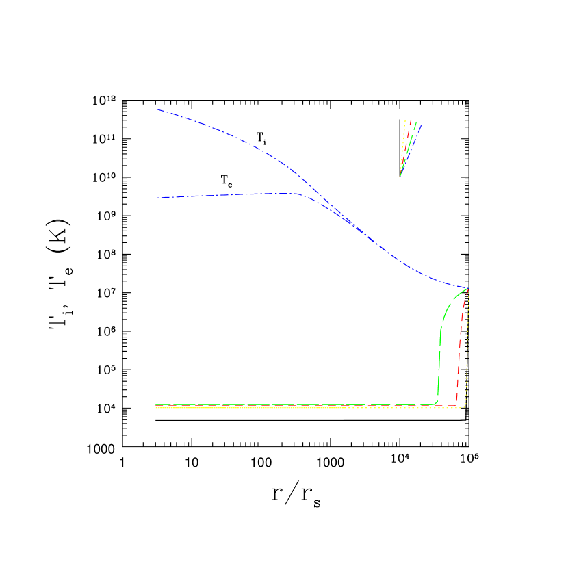
Figure 6: Ion ($T_{i}$) and electron ($T_{e}$) temperature profiles of $\dot{m}=0.01$, $M=10^{8}\,M_{\sun}$ un-preheated flow with equipartition magnetic field for given $\vartheta$’s. Solid line shows $T_{i}(r;\vartheta=0)=T_{e}(r;\vartheta=0)$, dotted line for $\vartheta=\pi/32$, short-dashed line for $\vartheta=\pi/16$, long-dashed line for $\vartheta=3\pi/32$, and dot-dashed lines for $\vartheta=\pi/8$ (upper one for ion and lower one for electron.) The profiles for larger $\vartheta$’s are almost same as those of $\vartheta=\pi/16$ case.

Figure 6 shows the typical temperature profiles of ions and electrons along different $\vartheta$ for the flow with equipartition magnetic field. Solid line shows ion and electron temperature profiles for $\vartheta=0$ (the polar axis) in ADAF with $\dot{m}=10^{-2}$. Up to $\vartheta=3\pi/32$ (long-dashed line), the flow stays near $10^{4}{\rm\,K}$ (dotted line for $\vartheta=\pi/32$ and short-dashed line for $\vartheta=\pi/16$). Because of the very small viscous and adiabatic heating near the polar axis, electrons cannot be maintained at a high temperature, and the stronger coupling between ions and electrons at lower electron temperature makes ions and electrons have the same temperatures at all radii for these $\vartheta$’s. Only for large enough $\vartheta$ (dot-dashed lines for $\vartheta=\pi/8$; upper one for ion and lower one for electron) ions and electrons maintain their high temperatures due to higher viscous heating rate and shorter flow time. As result we expect a conical region with $\vartheta\lesssim 3\pi/32$ around the polar axis will collapse while the flow along the equatorial plane accretes with significant radial velocity at high temperature. It is likely that the collapse would lead to an empty funnel along the polar axis. The temperature change across the surface of the funnel is going to be sudden, and the energy transfer by conduction may lead to further cooling from the hot part of the flow. But the existence and the generic shape of the funnel will remain the same. Of course this funnel may be filled by a tenuous outgoing wind, but consideration of this is beyond the scope of the present paper. However, the temperature profile of the flow near the equatorial plane agrees with the result from direct integration height-averaged equations with dynamics (Nakamura et al. 1997; Manmoto et al. 1997). Also, the flow remains at high temperatures for all values of mass accretion rate when the atomic cooling peak is intentionally removed, so it is clear that the effect we find (a collapse of the polar gas) is due to atomic cooling. In sum, it appears that for $\dot{m}>10^{-4}$ the ADAF solutions would collapse at the pole, with the funnel possibly filled with a tenuous hot outgoing wind.

We now turn to the cases where the temperature at the outer boundary is equal to the equilibrium temperature $\sim 10^{4}{\rm\,K}$. Because of the strong atomic cooling peak near $\sim 10^{4}{\rm\,K}$, electrons stay in this temperature until very strong heating takes over. For the same parameters as in $T(r_{out})=T_{vir}$ cases, we find that the flow is kept at $T_{i}=T_{e}\sim 10^{4}{\rm\,K}$ for all $\vartheta$ when the mass accretion rate $\dot{m}\gtrsim 2\times 10^{-4}$ (triangles in Fig. 5). The result differs significantly from the prior boundary condition $T(r_{out})=T_{vir}$ cases. This implies that only the very low mass accretion flow will reach the high temperature when the outer boundary is at $\sim 10^{4}{\rm\,K}$ and, therefore, the cool thin disk would not switch to hot a ADAF automatically for intermediate mass accretion rates unless there is some forcing process.

The luminosity and the radiation temperature (both at the outer boundary) of lower flow rate ($\dot{m}\lesssim 2\times 10^{-4}$) hot solutions for this boundary condition are shown in Figures 7 & 8, respectively, as diamonds. The dimensionless luminosity $l$ (diamonds in Fig. 7) for given dimensionless mass accretion rate $\dot{m}$ is about 100 times larger than that for the spherical accretion (Shapiro 1973b) because the density of ADAF is roughly 20–50 times (for $\alpha=0.1$ and $\epsilon^{\prime}=1$), depending on $\vartheta$, higher than the spherical flow with the same $\dot{m}$. The radiation temperature $T_{X}$ (diamonds in Fig. 8) is very low due to the copious soft synchrotron photons emitted (Shapiro 1973b). However, it increases as $\dot{m}$ approaches $10^{-3.7}$ because now lower temperature electrons mainly cool by bremsstrahlung. The sudden decrease of $l$ around $\dot{m}\simeq 2\times 10^{-4}$ in Figure 7 reflects the transition from hot ADAF to cold solutions as discussed above (triangles in Fig. 5). This transition does not depend on the strength of the magnetic field since it is mainly determined by the atomic cooling peak near $T\simeq 10^{4}{\rm\,K}$. For comparison, the detailed ADAF models for Sgr A^∗ ($M=2.5\times 10^{6}\,M_{\sun}$; Narayan et al. 1998) and NGC 4258 ($M=3.6\times 10^{7}\,M_{\sun}$; Lasota et al. 1996) are shown as $\earth$ and $\boxdot$ in Figures 7 and 8, respectively.

The luminosity and the radiation temperature of the flow without any magnetic field, thereby cooling only by Comptonized bremsstrahlung, are shown as stars in Figures 7 & 8. Due to the absence of soft synchrotron photons, the luminosity is much lower while the radiation temperature is much higher than the flow with magnetic field. An approximate effective temperature of the disk surface for the gas pressure dominated thin disk is shown as dotted line TD in Figure 8 for comparison.

When conditions of self-consistency (with regard to the thermodynamics of the emitted radiation) are applied to the solutions with $T(r_{out})=T_{eq}(r_{out})\simeq 10^{4}{\rm\,K}$, we see from Figure 8 that both the low and high temperature branches of the ADAF solutions are only possible for $\dot{m}\lesssim 10^{-3.7}$.

4.2 Preheated flow

PO suggested the possibility of preheated ADAF solutions, self-consistently maintained by the Compton preheating as in spherical accretion flows. These solutions are found by starting from ad hoc initial luminosity and radiation temperature high enough to affect the flow significantly (Park 1990a,b). Two dimensional plane of the luminosity and the radiation temperature, ($l$, $T_{X}$), is searched for the self-consistent values.

As in un-preheated flow, the outer boundary condition is important because the physical state of the flow inside depends on the entropy of the flow at the outer boundary. We have two possible choices: $T(r_{out})=T_{eq}(r_{out})\simeq 10^{4}{\rm\,K}$ or $T(r_{out})=T_{vir}(r_{out})$. In most cases, the latter condition is awkward because $T_{vir}(r_{out})$ is not the equilibrium temperature at $r_{out}$. The flow immediately adjusts to the equilibrium temperature $T_{eq}\simeq 10^{4}{\rm\,K}$ and stays at that temperature until much stronger heating brings the temperature up. The former choice, which is more natural in usual spherical accretion, unfortunately, is not consistent with the self-similar ADAF, where the sum of the ion pressure and the electron pressure is assumed to have the virial value. However, this choice would make joining the ADAF solutions to outer thin disk solution much more reasonable. So we adopt this boundary condition.

Figures 7 & 8 show the preheated solutions found in ($\dot{m}$,$l$) and ($\dot{m}$,$T_{X}$) plane, which may be called preheated ADAF (=PADAF). The circles represent the solutions with an exactly equipartition magnetic field. We find solutions sustained by preheating in the range $6.5\times 10^{-3}\lesssim\dot{m}\lesssim 0.15$, which includes the range in which no high temperature flow is possible when preheating is not considered ($\dot{m}>0.04$ or $\dot{m}>2\times 10^{-4}$). The luminosity of the preheated flow increases generally with the mass accretion rate (circles in Fig. 7). However, for $\dot{m}\lesssim 0.015$ the luminosity increases as the mass accretion rate decreases because the electron temperature reaches above $\sim 10^{9}{\rm\,K}$ for this low $\dot{m}$ flow, and synchrotron emission makes increasing contribution to the total luminosity. The majority of photons are now low energy synchrotron photons and the radiation temperature of these solutions decreases as $\dot{m}$ decreases and $l$ increases. This can be seen quite clearly in Figure 8. The radiation temperature decrease quite rapidly as $\dot{m}$ becomes smaller than $\sim 0.015$. Compared to the (un-preheated) ADAF, the PADAF has much higher radiation temperatures because most soft synchrotron photons are absorbed and inverse Comptonization is stronger. Solutions of NY3 are also shown (dotted line) in Figure 7 for comparison.

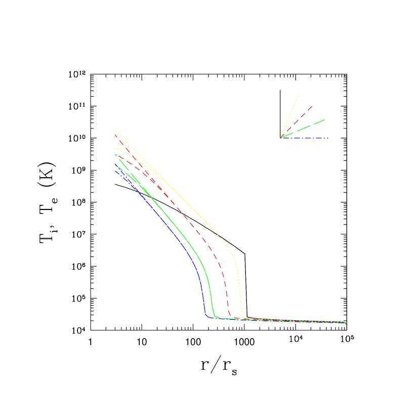
Figure 9: Ion ($T_{i}$) and electron ($T_{e}$) temperature profiles of PADAF with equipartition magnetic field for given $\vartheta$’s: $\dot{m}=0.01$ and $M=10^{8}\,M_{\sun}$ ($l=7.6\times 10^{-7}$, $T_{X}=1.2\times 10^{9}{\rm\,K}$). Now, solid line shows $T_{i}(r;\vartheta=0)=T_{e}(r;\vartheta=0)$, dotted lines for $\vartheta=\pi/8$, short-dashed lines for $\vartheta=\pi/4$, long-dashed lines for $\vartheta=3\pi/8$, and dot-dashed lines for $\vartheta=\pi/2$. Upper curves for ion temperature and lower ones for electron temperature.

The temperature profile of the typical PADAF solution is shown in Figure 9. The parameters of the flow are $\dot{m}=0.01$, $M=10^{8}\,M_{\sun}$, $l=4.1\times 10^{-6}$, and $T_{X}=1.2\times 10^{9}{\rm\,K}$. At the outer radii, the flow is kept near $10^{4}{\rm\,K}$. When the Compton heating becomes significant, the temperature suddenly jumps above $10^{6}{\rm\,K}$ first at the pole (solid line). This arises from the classic phase change due to the atomic cooling peak. Away from the pole, the density is higher, and the jump occurs at successively smaller radii. Also due to the faster infall velocity, the transition is smoother. Once the temperature is above $\gtrsim 10^{8}{\rm\,K}$, the Coulomb coupling gets weaker, and electron temperature deviates from that of the ions. The flow is mostly heated by Compton preheating by hot photons produced at smaller radii with added help of adiabatic compression and viscous heating. The electron temperature increases with varying slope at $T_{e}\gtrsim 10^{9}{\rm\,K}$ by relativistic effects and then flattens due to highly efficient Comptonized relativistic bremsstrahlung and Comptonized synchrotron radiation at this temperature range.

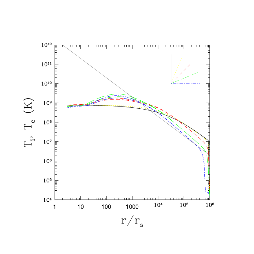
Figure 10: Same as Figure 9 but for $\dot{m}=0.15$, $M=10\,M_{\sun}$ ($l=1.0\times 10^{-3}$, $T_{X}=8.2\times 10^{8}{\rm\,K}$) WADAF. Thin solid line shows the virial temperature.

Now we look at a higher $\dot{m}$, higher $l$ solution (Fig. 10 for $\dot{m}=0.1$, $M=10\,M_{\sun}$). Due to the higher density, ions and electrons are well coupled. The flow in the polar axis (solid line) is heated first at much larger radii compared to lower $\dot{m}$ flow, and larger $\vartheta$ flow is heated successively (dotted line for $\vartheta=\pi/8$, short-dashed line for $\vartheta=\pi/4$, long-dashed line for $\vartheta=3\pi/8$, and dot-dashed line for $\vartheta=\pi/2$). Note that within the radius range $10^{3}<r/r_{s}<10^{6}$, the flow temperature of the polar region is much greater than the virial temperature (thin solid line) while that for the equatorial plane (dot-dashed line) is close to the virial value. This will produce the preheating instability or wind preferentially along the pole as suggested in PO because longer infall timescale along the pole makes this part of the flow more vulnerable to instability while shorter infall timescale near the equatorial plane stabilizes the flow. We may call this type of solutions ADAF with polar wind (WADAF). So, preheating may be yet another process to produce outflow in ADAF (Xu & Chen 1997; Blandford & Begelman 1999; Das 1999; Turolla & Dullemond 2000; see also Menou et al. [1999] for the polar wind in neutron star accretion). Meanwhile, if the mass accretion rate, and accordingly the luminosity also, is much higher, all parts of the flow will be heated well above the virial value. Since in spherical flow overheating outside the sonic point produces long term modulation on the accretion rate and that inside the sonic point produces short term flaring (Cowie et al. 1978), it is likely that these higher $l$ flow may develop either a relaxational variability or a flaring variability.

The range of $\dot{m}$ to have equatorial accretion and the preheated polar outflow simultaneously is rather limited around $\dot{m}\simeq 0.15$. This range will be wider for larger $\epsilon^{\prime}$ and narrower for smaller $\epsilon^{\prime}$, because larger $\epsilon^{\prime}$ flow has a higher density contrast between the pole and the equator.

When there is no magnetic field, Comptonized bremsstrahlung is the only cooling process, and the properties of these flow show more continuous behavior (crosses in Figs. 7 & 8). They also exist in a wider $\dot{m}$ range, $10^{-3.5}\lesssim\dot{m}\lesssim 10^{-1}$. The slope of $l$ versus $\dot{m}$ changes around $\dot{m}\simeq 10^{-2}$ because the electrons can reach near $10^{9}{\rm\,K}$, and relativistic radiative process becomes important.

5 Summary and Discussion

We have studied the two-dimensional thermal properties of the ADAF by integrating the energy equations under the assumption that the density and velocity of the flow is described by the self-similar solutions of Narayan & Yi (1995a). Special considerations are given to the effects of preheating by Comptonizing hot photons produced at smaller radii and radiative transfer of these photons, as well as to the atomic cooling, Comptonized relativistic bremsstrahlung, and Comptonized synchrotron radiation. We find that Compton preheating is important in general.

1. When preheating is not considered, the high temperature flows do not exist when the mass accretion rate is higher than $\sim 10^{-1.5}L_{E}c^{-2}$, and even below this mass accretion rate, a roughly conical region around the hole cannot sustain high temperature ions and electrons. Funnels should exist in these flows unless $\dot{m}\equiv\dot{M}c^{2}/L_{E}<10^{-4}$. If the flow starts at large radii with a normal equilibrium temperature $\sim 10^{4}{\rm\,K}$ as in spherical flows, the critical mass accretion rate becomes $\dot{m}\sim 10^{-3.7}$, above which level no self-consistent solutions exist.

2. Even above this critical mass accretion rate, the flow can be self consistently maintained at high temperature if Compton preheating is considered. These solutions constitute a new branch of solutions as in the case of spherical accretion flow; these preheated high temperature ADAFs can exist above the critical mass accretion rate in addition to the usual cold thin disk. Therefore, Compton preheating could be the mechanism to trigger the phase change from the thin disk to PADAF—the preheated ADAF.

3. We also find solutions where the flow near the equatorial plane is normally accreting while that near the polar axis is overheated by Compton preheating, possibly becoming polar wind. The flow may be called WADAF—ADAF with a polar wind.

The formalism we have used in this work is not completely satisfactory in the sense that the dynamics of the flow is prescribed to be ADAF like. In real flow, changes in thermal properties will induce those in dynamical properties. Hence, although solving the two dimensional flow structure with the correct radiative transfer is a daunting task, understanding the true nature of the ADAF like solutions seems to demand it. We feel confident, however, that the characteristic solutions for all accretion rates of interest ($\dot{m}\gtrsim 10^{-3}$) will be either PADAF or WADAF type when the outer boundary approaches the equilibrium ($T\sim 10^{4}{\rm\,K}$) temperature.

Appendix A Cooling and heating processes

A.1 Atomic cooling and bremsstrahlung

Cooling due to atomic processes and bremsstrahlung is expressed as a composite formula (Svensson 1982; Stepney & Guilbert 1983; Nobili et al. 1991)

$$\Lambda_{Cbr+atomic}=\sigma_{T}c\alpha_{f}m_{e}c^{2}n_{i}^{2}\Big{[}\big{\{}\lambda_{Cbr}(T_{e})+6.0\times 10^{-22}\theta_{e}^{-1/2}\big{\}}^{-1}+\left(\frac{\theta_{e}}{4.82\times 10^{-6}}\right)^{-12}\Big{]}^{-1},$$ (A1)

where $\sigma_{T}$ is the Thomson cross section, $\alpha_{f}$ the fine-structure constant, and $n_{i}$ the number density of ions. In part of the flow with high temperature where most of the radiation is produced, the bremsstrahlung cooling rate is not much affected by free-free absorption because most energies are carried by photons with energy $\sim kT_{e}$ in bremsstrahlung emission.

The cooling rate due to the Comptonized bremsstrahlung $\Lambda_{Cbr}$ can be expressed as some average enhancement factor times the un-Comptonized bremsstrahlung rate

$$\lambda_{br}=\left(\frac{n_{e}}{n_{i}}\right)(\sum_{i}Z_{i}^{2})F_{ei}(\theta_{e})+\left(\frac{n_{e}}{n_{i}}\right)^{2}F_{ee}(\theta_{e})$$ (A2)

where

$$F_{ei} = 4\left(\frac{2}{\pi^{3}}\right)^{1/2}\theta_{e}^{1/2}(1+1.781\theta_{e}^{1.34})\quad\hbox{for}~{}~{}\theta_{e}<1$$

$$= \frac{9}{2\pi}\theta_{e}\left[\ln(1.123\theta_{e}+0.48)+1.5\right]\quad\hbox{for}~{}~{}\theta_{e}>1$$

$$F_{ee} = \frac{5}{6\pi^{3/2}}(44-3\pi^{2})\theta_{e}^{3/2}(1+1.1\theta_{e}+\theta_{e}^{2}-1.25\theta_{e}^{5/2})\quad\hbox{for}~{}~{}\theta_{e}<1$$

$$= \frac{9}{\pi}\theta_{e}\left[\ln(1.123\theta_{e})+1.2746\right]\quad\hbox{for}~{}~{}\theta_{e}>1.$$

Obtaining a precise estimate of the enhancement factor for arbitrary optical depth, electron temperature, and flow geometry is a quite formidable task by itself. However, Dermer, Liang, & Canfield (1991) provide a convenient, yet reasonable way to deal with thermal Comptonization. They define a Comptonized energy enhancement factor $\eta(\nu)$ as the average change in photon energy between creation and escape in a flow with an electron scattering optical depth $\tau_{es}$ and electron temperature $T_{e}$,

$$\eta(\nu)=1+\eta_{1}-\eta_{2}\left(\frac{x}{\theta_{e}}\right)^{\eta_{3}}$$ (A5)

where $x\equiv h\nu/m_{e}c^{2}$, $P=1-\exp(-\tau_{es})$, $A=1+4\theta_{e}+16\theta_{e}^{2}$, $\eta_{1}\equiv P(A-1)/(1-PA)$, $\eta_{3}\equiv-1-\ln P/\ln A$, and $\eta_{2}\equiv\eta_{1}/3^{\eta_{3}}$. Although this formula is not applicable to certain ranges of $\nu$ and $\tau_{es}$, it is good enough for general use.

We apply $\eta(\nu)$ to the bremsstrahlung spectrum

$$\epsilon_{br}(x)d\left(\frac{x}{\theta_{e}}\right)=\Lambda_{br}\exp\left(-\frac{x}{\theta_{e}}\right)d\left(\frac{x}{\theta_{e}}\right)$$ (A6)

to get the Comptonized bremsstrahlung cooling rate. When absorption is not important, photon with energy $x$ ($x\lesssim 3\theta_{e}$) would be upscattered to $\eta x$, and the cooling rate would be

$$\Lambda_{Cbr} = \int_{0}^{3\theta_{e}}\eta x\frac{\epsilon_{br}}{x}dx+\int_{3\theta_{e}}^{\infty}\epsilon_{br}(x)dx$$ (A7)

$$= \int_{0}^{\infty}\epsilon_{br}(x)dx+\int_{0}^{3\theta_{e}}(\eta-1)\epsilon_{br}(x)dx.$$ (A8)

For the second integration, we use simpler form of $\epsilon_{br}$,

$$\epsilon_{br}^{0}(x)d\left(\frac{x}{\theta_{e}}\right) = \Lambda_{br}d\left(\frac{x}{\theta_{e}}\right)\quad x\leq\theta_{e}$$ (A9)

$$= 0\quad\quad\quad x>\theta_{e}$$ (A10)

since very little emission exists above $x>\theta_{e}$. The resulting cooling rate is

$$\Lambda_{Cbr}=\Lambda_{br}\left[1+\eta_{1}-\frac{\eta_{2}}{\eta_{3}+1}\right].$$ (A11)

When $\theta_{e}$ and $\tau_{es}$ increases such that $PA\sim 1$, most photons are likely to be upscattered to $\sim kT_{e}$. Equation (A5) has a formal divergence in this saturated Comptonization regime. If we assume that photons with energy above $h\nu_{abs}$ are all upscattered to $kT_{e}$, the saturated energy enhancement factor for the whole emission is

$$\Lambda_{Cbr}^{sat}/\Lambda_{br} = 1+\int_{x_{abs}}^{\theta_{e}}\frac{3\theta_{e}}{x}d\left(\frac{x}{\theta_{e}}\right)$$ (A12)

$$= 1+3\ln\left(\frac{\theta_{e}}{x_{abs}}\right).$$ (A13)

Hence, the Comptonized bremsstrahlung cooling rate in general is

$$\Lambda_{Cbr}^{sat}=\Lambda_{br}\min\left[1+\eta_{2}-\frac{\eta_{2}}{\eta_{3}+1},1+3\ln\big{(}\frac{\theta_{e}}{x_{abs}}\big{)}\right].$$ (A14)

The energy-weighted mean photon energy for the emission is expressed as

$$\frac{kT_{S}^{Cbr}}{m_{e}c^{2}} = \Lambda_{Cbr}^{-1}\int_{0}^{\infty}(\eta x)^{2}\frac{\epsilon_{br}}{x}dx$$ (A15)

$$\simeq \int_{0}^{\infty}x\epsilon_{br}(x)dx+\int_{0}^{\theta_{e}}(\eta^{2}-1)x\epsilon_{br}^{0}(x)dx$$ (A16)

$$= \theta_{e}\frac{\Lambda_{br}}{\Lambda_{Cbr}}\left[1+\eta_{1}(\eta_{1}+2)-\frac{2\eta_{2}(1+\eta_{1})}{\eta_{3}+2}+\frac{\eta_{2}^{2}}{2\eta_{3}+1}\right].$$ (A17)

Since this expression has divergence near saturated regime, we put an upper limit $T_{S}=T_{e}$ (Wien spectrum),

$$T_{S}^{Cbr}=\text@frac{1}{4}kT_{e}\min\left[4,\frac{1+\eta_{1}(\eta_{1}+2)-\frac{2\eta_{2}(1+\eta_{1})}{\eta_{3}+2}+\frac{\eta_{2}^{2}}{2\eta_{3}+1}}{1+\eta_{1}-\frac{\eta_{2}}{\eta_{3}+1}}\right]$$ (A18)

which has a limit value $T_{S}^{Cbr}=\text@frac{1}{4}T_{e}$ when Comptonization is negligible.

A.2 Synchrotron

Even an equipartition magnetic field does not play an important role in dynamics of spherical accretion (Shapiro 1974). But synchrotron emission could be the dominant cooling process nevertheless. In this work we assume a magnetic field of the order of equipartition strength:

$$P_{m}=\frac{B^{2}}{24\pi}=\beta(P_{g}+P_{m})=\beta P$$ (A19)

where $P_{m}$ is the magnetic pressure, $P_{g}$ the gas pressure, and $P$ the total pressure.

The angle-averaged synchrotron emission by relativistic Maxwellian electrons is given by (Pacholczyk 1970)

$$\epsilon_{syn}=\frac{2\pi}{\sqrt{3}}\frac{e^{2}}{c}\frac{n_{e}\nu}{\theta_{e}^{2}}I^{\prime}(x_{M})d\nu$$ (A20)

where $x_{M}\equiv 2\nu/(3\nu_{0}\theta_{e}^{2})$, $\nu_{0}\equiv eB/(2\pi m_{e}c)$, and

$$I^{\prime}(x_{M})=\frac{4.0505}{x_{M}^{1/6}}\left(1+\frac{0.40}{x_{M}^{1/4}}+\frac{0.5316}{x_{M}^{1/2}}\right)\exp(-1.8899x_{M}^{1/3})$$ (A21)

is a fitting formula (Mahadevan, Narayan, & Yi 1996).

When absorption is not important, the cooling rate due to the optically thin synchrotron emission is obtained by integrating the equation (A20)

$$\Lambda_{syn}^{0}=213.6\frac{e^{2}}{c}n_{e}\nu_{0}^{2}\theta_{e}^{2}.$$ (A22)

In generic accretion flow, a large fraction of the low energy synchrotron photons can be absorbed either by synchrotron self-absorption or by free-free absorption, and its effect should be incorporated along with that of Comptonization.

If the flow becomes optically thick in absorption at frequency $\nu_{abs}$, the synchrotron cooling (before Comptonization) can be expressed as

$$\Lambda_{syn}=f_{syn}\Lambda_{syn}^{0}$$ (A23)

where

$$f_{syn}\equiv\int_{x_{abs}}^{\infty}xI^{\prime}(x)dx\Big{/}\int_{0}^{\infty}xI^{\prime}(x)dx$$ (A24)

and $x_{abs}=h\nu_{abs}/m_{e}c^{2}$. By this, we assume all photons above $\nu_{abs}$ escape the gas flow. The treatment of cooling when the flow is optically thick to absorption for lower energy photons and thin for higher energy ones can be tricky because the absorbed radiation heats the gas and the slight difference in the radiation field between two different radii drives the transfer of the energy while higher energy photons directly escape. Correct calculation of this would require solving gas energy equations and radiative transfer equations with frequency dependence. A simpler way would be to consider only the photons that escape as the source of cooling (Ipser & Price 1982), neglecting the diffusive cooling due to the absorbed photons, which we adopt here (see NY3 for different approach).

For Comptonization of absorbed synchrotron photons, we assume that photons near the cut-off frequency $\sim\nu_{abs}$ are most affected by Comptonization, and the cooling rate due to the Comptonization of synchrotron photons is simply

$$\Lambda_{Csyn}=\eta(\nu_{abs})f_{syn}\Lambda_{syn}^{0}.$$ (A25)

Similarly, the radiation temperature of the Comptonized synchrotron photons, $T_{S}^{syn}$, is

$$4kT_{S}^{syn}=h\nu_{abs}\eta(\nu_{abs}).$$ (A26)

A.3 Absorption

There are two sources of absorption: free-free and synchrotron self-absorption. At high temperature where most of the radiation is produced, synchrotron absorption is more important in general. In this work, we estimate the frequency at which either absorption is important under the effect of Comptonization, and use the larger of the two as $\nu_{abs}$.

The difficulty of considering absorption under Comptonization is that a photon having a big chance of being absorbed in the absence of Comptonization can be upscattered and its mean free path for absorption can increase, resulting in escape before being absorbed. So the effective frequency where absorption becomes important becomes lower due to Compton scattering. This would be far more important to synchrotron losses than to bremsstrahlung because most of emission in synchrotron radiation is in the tail part of the spectrum and the precise location of the absorption frequency can change the emission by some exponential factor.

Dermer, Liang, & Canfield (1991) estimate the effective absorption frequency by equating the characteristic timescale for absorption with that for the energy increase due to Compton scattering in case of free-free absorption. We apply this approach to both free-free absorption and synchrotron self-absorption.

The absorption frequency $\nu_{abs}^{ff}$ for free-free absorption is estimated from the relation (Dermer, Liang, & Canfield 1991)

$$\tau_{ff}(\nu_{abs}^{ff})\Upsilon=1$$ (A27)

where $\tau_{ff}=ra_{ff}$ and $a_{ff}$ is the absorption coefficient

$$a_{ff}(x)=\sqrt{8\pi}\frac{\alpha_{f}^{2}\sigma_{T}r_{e}^{3}}{x^{2}\theta_{e}^{3/2}\left[1+(8/\pi)^{1/2}\theta_{e}^{3/2}\right]}n_{i}^{2}\bar{g}$$ (A28)

and

$$\bar{g} = (1+3Y_{He})(1+2\theta_{2}+2\theta_{e}^{2})\ln\left[\frac{4\eta_{E}(1+3.42\theta_{e})\theta_{e}}{x}\right]$$

$$+(1+Y_{He}^{2})(\frac{3\sqrt{2}}{5}+2\theta_{2})\theta_{e}\ln\left[\frac{4\eta_{E}(11.2+10.4\theta_{e}^{2})\theta_{e}}{x}\right],$$

$\alpha_{f}$ the fine structure constant, and $r_{e}=e^{2}/m_{e}c^{2}$ the electron radius (Svensson 1984). This expression is valid for $x\ll\theta_{e}$ and we used $\sqrt{\pi/2}\theta_{e}^{1/2}[1+(8/\pi)^{1/2}\theta_{e}^{3/2}]$ to approximate $\exp(1/\theta_{e})\hbox{K}_{2}(1/\theta_{e})$. The factor $\Upsilon$ includes the effect of Comptonization,

$$\Upsilon = \frac{1}{\min[1,8\theta_{e}]\tau_{es}}\quad\hbox{if}~{}~{}y>1~{}~{}\hbox{and}~{}~{}\tau_{es}>1$$ (A30)

$$= 1+\xi\tau_{es}\quad\quad\quad\hbox{otherwise}$$ (A31)

where $\xi=1/3$ is the geometry factor and $y\equiv(4\theta_{e}+16\theta_{e}^{2})\max[\tau_{es},\tau_{es}^{2}]$ is the usual Compton parameter.

The absorption frequency $\nu_{abs}^{syn}$ for synchrotron self-absorption is similarly calculated (Svensson 1984; Dermer, Liang, & Canfield 1991),

$$\tau_{syn}(\nu_{abs}^{syn})\Upsilon=1$$ (A32)

where

$$\tau_{syn}=\frac{1}{4\sqrt{3}}\frac{e^{2}cn_{e}r}{\nu kT_{e}\theta_{e}^{2}}I^{\prime}(x_{M})$$ (A33)

(Ipser & Price 1982; Mahadevan, Narayan, & Yi 1996).

Then, the effective absorption frequency $\nu_{abs}$ is set to be the maximum of $\nu_{abs}^{ff}$ and $\nu_{abs}^{syn}$.

A.4 Viscous heating

The ion heating rate per unit volume under $\alpha$-viscosity description (Shakura & Sunyaev 1973) is (NY2)

$$\Gamma_{vis}=\alpha\rho c_{s}^{2}\Omega_{K}\left[3v^{2}(\vartheta)+\text@frac{9}{4}\Omega^{2}(\vartheta)\sin^{2}\vartheta+\big{(}\frac{\partial v(\vartheta)}{\partial\vartheta}\big{)}^{2}+\sin^{2}\vartheta\big{(}\frac{\partial\Omega(\vartheta)}{\partial\vartheta}\big{)}^{2}\right].$$ (A34)

A.5 Compton heating

We now turn to process which can be dispositive in disrupting accretion flow. Electrons in outer regions, $r/r_{s}\sim 10^{4}\rightarrow 10^{5}$, can be heated by high-energy photons produced at inner hot region, $r/r_{s}\sim 10^{1}\rightarrow 10^{2}$, of the flow. We use Compton heating rate from the Kompaneets equation (Levich & Syunyaev 1971; Rybicki & Lightman 1979),

$$\Gamma_{Compt}=n_{e}\sigma_{T}\frac{4k[T_{X}(r)-T_{e}(r)]}{m_{e}c^{2}}\frac{L_{X}(r)}{4\pi r^{2}}.$$ (A35)

The information on the preheating radiation spectrum is incorporated in the angle-averaged quantities, $T_{X}(r)$ and $L_{X}(r)$, which are calculated from the equations (11) and (13) along with corresponding auxiliary equations.

Figure 1: Spherical and disk accretion flow solutions in ($l$, $\dot{m}$) plane [$l\equiv L/L_{E}$, $\dot{m}\equiv\dot{M}c^{2}/L_{E}$]. Solid line S represents low $\dot{m}$ spherical accretion solutions of Shapiro (1973a), large crosses are those of Park (1990b). Low temperature solutions of high $\dot{m}$ spherical accretion are triangles (Nobili et al. 1991) and high temperature solutions are large open circles (Park 1990b). Accretion disk solutions appear as dotted line TD for thin disk, dot-dashed line SD for slim disk, and dashed line NY for ADAF (NY3). Spherical accretion solutions with electron-positron pairs are small filled circles (Park & Ostriker 1989), those with the magnetic field reconnection small squares, and those with preheating shocks small crosses (Chang & Ostriker 1989).

Figure 2: The radiation temperature $T_{X}(r_{out})$ (in K) of the self-consistent spherical solutions. Symbols are the same as in Figure 1. Note that the non magnetic high and low temperature solutions (crosses and triangles) are quite distinct on this plane, but continuous in Figure 1. The separate branch of the self-consistent high temperature, high-luminosity flows (circles) exists also in the ADAF case (PADAF).

Figure 3: Spherical and disk accretion flow solutions in ($l$, $e$) plane [$e\equiv L/\dot{M}c^{2}$]. Symbols are the same as in Figure 1. Note that all of the physically thick, self-consistent solutions expected or known to be stable (crosses, triangles, and circles) have an efficiency $\lesssim 10^{-4}$.

Figure 4: Various accretion disk solutions in accretion rate $\dot{m}$ versus surface mass density $\Sigma$ (in arbitrary units) plane: ADAF for ADAFs, SLE for high temperature, geometrically thin disk solutions, SD for slim disk solutions, RTD for radiation pressure dominated thin disk solutions, and GTD for gas pressure dominated thin disk solutions.

Figure 5: For the branch of the ADAF solutions for which preheating is not important, we plot the angle of the conical region (in degree) around the polar axis where the temperature of the flow is $\sim 10^{4}{\rm\,K}$ as a function of $\dot{m}$. Circles for boundary condition $T(r_{out})=T_{vir}(r_{out})$ and triangles for $T(r_{out})=T_{eq}(r_{out})$. With the specified cone angle pressure balance cannot be maintained and a conical hole would appear. Thus no solution is possible for $\dot{m}$ above the limiting points indicated by the filled symbols.

Figure 7: The dimensionless luminosity $L(r_{out})/L_{E}$ of solutions found in this work for accretion onto $10\,M_{\sun}$ black hole. Circles and diamonds are those with equipartition magnetic field, and crosses and stars are those without magnetic field. Diamonds and stars are ADAFs where preheating is negligible while circles and crosses are ADAFs maintained by preheating (PADAF). Filled circle represent ADAF with polar wind (WADAF). One dimensional ADAF solutions (NY3) are shown as dotted line. Detailed ADAF models for Sgr A^∗ ($M=2.5\times 10^{6}\,M_{\sun}$) and NGC 4258 ($M=3.6\times 10^{7}\,M_{\sun}$) are shown as $\earth$ and $\boxdot$, respectively. ADAFs with equipartition magnetic field are not permitted in the shaded region.

Figure 8: The radiation temperature $T_{X}(r_{out})$ (in ${\rm\,K}$) of solutions found in this work for accretion onto $10\,M_{\sun}$ black hole with $T(r_{out})\simeq 10^{4}{\rm\,K}$. Symbols are same as in Figure 7. The effective temperature of the thin disk surface is shown as dotted line TD. Note that without preheating there are no self-consistent ADAF solutions with $\dot{m}\gtrsim 10^{-3.7}$.

References

- (1)
- (2) Abramowicz, M., Chen, X., Kato, S., Lasota, J.-P., & Regev, O. 1995, ApJ, 438, L37
- (3) Abramowicz, M. A., Czerny, B., Lasota, J.-P., & Szuszkiewicz, E. 1988, ApJ, 332, 646
- (4) Abramowicz, M. A., Calvani, M., & Nobili, L. 1980, ApJ, 242, 772
- (5) Begelman, M. C. 1978, MNRAS, 184, 53
- (6) Bisnovatyi-Kogan, G. S., & Blinnikov, S. I. 1980, MNRAS, 191, 711
- (7) Blandford, R. D. & Begelman, M. C. 1999, MNRAS, 303, L1
- (8) Blondin, J. M. 1986, ApJ, 308, 755
- (9) Bondi, H. 1952, MNRAS, 112, 195
- (10) Bondi, H. & Hoyle, F. 1944, MNRAS, 104, 273
- (11) Chakrabarti, S. K. 1996a, ApJ, 464, 664
- (12) Chakrabarti, S. K. 1996b, Phys. Rep., 266, 238
- (13) Chang, K. M. & Ostriker, J. P. 1985, ApJ, 288, 428
- (14) Chen, X., Abramowicz, M. & Lasota, J.-P. 1997, ApJ, 476, 61
- (15) Chen, X., Abramowicz, M., Lasota, J.-P., Narayan, R., & Yi, I. 1995, ApJ, 443, L61
- (16) Chen, X. Taam, R. E., Abramowicz, M. A., & Igumenshchev, I. V. 1997, MNRAS, 285, 439
- (17) Choi, Y., Yang, J., & Yi, I. 1999, ApJ, 518, L77
- (18) Ciotti, L., & Ostriker, J. P. 1997, ApJ, 487, L105
- (19) Ciotti, L., & Ostriker, J. P. 1999, preprint (astro-ph/9912064)
- (20) Cowie, L. L., Ostriker, J. P., and Stark, A. A. 1978, ApJ, 226, 1041
- (21) Das, T. K. 1999, MNRAS, 308, 201
- (22) Dermer, C. D., Liang, E. P., & Canfield, E. 1991, ApJ, 369, 410
- (23) Di Matteo, T. & Fabian, A. C. 1997, MNRAS, 286, L50
- (24) Esin, A. A. 1997, ApJ, 482, 400
- (25) Flamang, R. A. 1982, MNRAS, 199, 833
- (26) Flamang, R. A. 1984, MNRAS, 206, 589
- (27) Frank, J., King, A., & Raine, D. 1992, Accretion Power in Astrophysics (Cambridge: Cambridge Univ. Press)
- (28) Gammie, C. F. & Popham, R. 1998, ApJ, 498, 313
- (29) Grindlay, J. E. 1978, ApJ, 221, 234
- (30) Hoyle, F. & Lyttleton, R. A. 1939, Proc. Camb. Phil. Soc., 35, 405
- (31) Igumenshchev, I. V. & Abramowicz, M. A. 1999, MNRAS, 303, 309
- (32) Igumenshchev, I. V. & Beloborodov, A. M. 1997, MNRAS, 284, 767
- (33) Ichimaru, S. 1977, ApJ, 214, 840
- (34) Ipser, J. R. & Price, R. H. 1982, ApJ, 255, 654
- (35) Jaroszyński, M., Abramowicz, M. A., & Paczyński, B. 1980, Acta Astron., 255, 654
- (36) Krolik, J. H., & London, R. A. 1983, ApJ, 267, 18
- (37) Kusunose, M. & Mineshige, S. 1992, ApJ, 392, 653
- (38) Lasota, J.-P., Abramowicz, M. A., Chen, X., Krolik, J., Narayan, R., & Yi, I. 1996, ApJ, 462, 142
- (39) Levich, E. V. & Syunyaev R. A. 1971, Soviet Ast., 15, 363
- (40) Lightman, A. P., & Eardley, D. M. 1974, ApJ, 187, L1
- (41) Loeb, A. & Laor, A. 1992, ApJ, 384, 115
- (42) Lu, J.-F., Gu, W.-M., & Yuan, F. 1999, ApJ, 523, 340
- (43) Mahadevan, R. 1997, ApJ, 477, 585
- (44) Mahadevan, R., Narayan, R., & Krolik, J. 1997, ApJ, 486, 268
- (45) Mahadevan, R., Narayan, R., & Yi, I. 1996, ApJ, 465, 327
- (46) Manmoto, T., Mineshige, S., & Kusunose, M. 1997, ApJ, 489, 791
- (47) Maraschi, L., Roasio, R., & Treves, A. 1982, ApJ, 253, 312
- (48) Mason, A. & Turolla, R. 1992, ApJ, 400, 170
- (49) Melia, F. 1992, ApJ, 387, L25
- (50) Melia, F. 1994, ApJ, 426, 577
- (51) Menou, K., Esin, A. A., Narayan, R., Garcia, M. R., Lasota, J. -P., & McClintock, J. E. 1999, ApJ, 520, 276
- (52) Mészáros, P. 1975, A&A, 44, 59
- (53) Mihalas, D. & Mihalas, B. W. 1984, Foundations of Radiation Hydrodynamics (Oxford: Oxford Univ. Press)
- (54) Miller, G. S. 1990, ApJ, 356, 572
- (55) Molteni, D., Lanzafame, G. & Chakrabarti, S. K. 1994, ApJ, 425, 161
- (56) Nakamura, K. E., Kusunose, M., Matsumoto, R., & Kato, S. 1997, PASJ, 49, 503
- (57) Narayan, R., Barret, D., & McClintock, J. E. 1997, ApJ, 482, 448
- (58) Narayan, R., Kato, S., & Honma, F. 1997, ApJ, 476, 49
- (59) Narayan, R., Mahadevan, R., Grindlay, J. E., Popham, R. G., & Gammie, C. 1998a, ApJ, 492, 554
- (60) Narayan, R., Mahadevan, R., & Quataert 1998b, in The Theory of Black Hole Accretion Discs, eds. M. A. Abramowicz, G. Bjornsson, and J. E. Pringle (Cambridge: Cambridge U. Press)
- (61) Narayan, R., McClintock, J. E., & Yi, I. 1996, ApJ, 457, 821
- (62) Narayan, R. & Yi, I. 1994, ApJ, 428, L13 (NY1)
- (63) Narayan, R. & Yi, I. 1995a, ApJ, 444, 231 (NY2)
- (64) Narayan, R. & Yi, I. 1995b, ApJ, 452, 710 (NY3)
- (65) Narayan, R., Yi, I., & Mahadevan, R. 1995, Nature, 374, 623
- (66) Novikov, I. D., & Thorne, K. S. 1973, in Black Holes, ed. C. DeWitt & B. DeWitt (New York: Gordon & Breach), 343
- (67) Nobili, L., Turolla, R., & Zampieri, L. 1991, ApJ, 383, 250
- (68) Ostriker, J. P., McCray, R., Weaver, R., & Yahil, A. 1976, ApJ, 208, L61
- (69) Quataert, E., & Narayan, R. 1999, ApJ, 516, 399
- (70) Pacholczyk, A. G. 1970, Radio Astrophysics (San Francisco: Freeman)
- (71) Paczyński, B. 1998, Acta Astron., 48, 667
- (72) Paczyński, B. & Wiita, P. 1980, A&A, 88, 23
- (73) Park, M.-G. 1990a, ApJ, 354, 64
- (74) Park, M.-G. 1990b, ApJ, 354, 83
- (75) Park, M.-G. 1993, A&A, 274, 642
- (76) Park, M.-G. 1995, J. of Korean Ast. Soc., 28, 97
- (77) Park, M.-G. & Miller, G. S. 1991, 371, 708
- (78) Park, M.-G. & Ostriker, J. P. 1989, ApJ, 347, 679
- (79) Park, M.-G. & Ostriker, J. P. 1999, ApJ, 527, 247 (PO)
- (80) Piran, T. 1978, ApJ, 221, 652
- (81) Popham, R. & Gammie, C. F. 1998, ApJ, 504, 419
- (82) Pringle, J. E. 1976, MNRAS, 177, 65
- (83) Pringle, J. E. 1981, ARA&A, 19, 137
- (84) Pringle, J. E., & Rees, M. J. 1973, A&A, 21, 1
- (85) Rees, M. J., Begelman, M. C., Blanford, R. D., & Phinney, E. S. 1982, Nature, 295, 17
- (86) Rybicki, G. B. & Lightman, A. P. 1979, Radiative Processes in Astrophysics (New York: Wiley)
- (87) Ryu, D, Brown, G. L., Ostriker, J. P., & Loeb, A. 1995, ApJ, 452, 364
- (88) Service, A. T. 1986, ApJ, 307, 60
- (89) Shakura, N. I. 1972, Astron. Zh., 49, 921 (1973, Sov. Astron., 16, 756)
- (90) Shakura, N. I., & Sunyaev, R. A. 1973, A&A, 24, 337
- (91) Shakura, N. I., & Sunyaev, R. A. 1976, MNRAS, 175, 613
- (92) Shapiro, S. L. 1973a, ApJ, 180, 531
- (93) Shapiro, S. L. 1973b, ApJ, 185, 69
- (94) Shapiro, S. L. 1974, ApJ, 189, 343
- (95) Shapiro, S. L., Lightman, A. P., & Eardley, D. N. 1976, ApJ, 204, 187
- (96) Spruit, H. C., Matsuda, T, Inoue, M., & Sawada, K. 1987, MNRAS, 229, 517
- (97) Stellingwerf, R. F., & Buff, J. 1982, ApJ, 260. 755
- (98) Stepney, S. 1983, MNRAS, 202, 467
- (99) Stepney, S., & Guilbert, P. W. 1983, MNRAS, 204, 1269
- (100) Stone, J. M., Pringle, J. E., & Begelman, M. C. 1999, preprint (astro-ph/9908185)
- (101) Svensson, R. 1982, ApJ, 258, 335
- (102) Svensson, R. 1984, MNRAS, 209, 175
- (103) Szuszkiewicz, E., Malkan, M. A. & Abramowicz, M. A. 1996, ApJ, 458, 474
- (104) Treves, A, Maraschi, L., Abramowicz, M. 1988, PASP, 100, 427
- (105) Turolla, R., & Dullemond, C. P. 2000, preprint (astro-ph/0001114)
- (106) Wandel, A., Yahil, A., & Milgrom, M. 1984, ApJ, 282, 53
- (107) Wu, X.-B. 1997, MNRAS, 292, 113
- (108) Xu, G. & Chen, X. 1997, ApJ, 489, L29
- (109) Yi, I. 1996, ApJ, 473, 645
- (110) Yi, I. & Boughn, S. 1998, ApJ, 499, 198
- (111) Yi, I., & Narayan, R. 1997, ApJ, 486, 363
- (112) Yi, I. & Wheeler, J. C. 1998, ApJ, 498, 802
- (113) Zampieri, L., Miller, J. C., & Turolla, R. 1996, MNRAS, 281, 1183
- (114)