Estimating reaction rates and uncertainties for primordial nucleosynthesis

Abstract

We present a Monte Carlo method for direct incorporation of nuclear inputs in primordial nucleosynthesis calculations. This method is intended to remedy shortcomings of current error estimation, by eliminating intermediate data evaluations and working directly with experimental data, allowing error estimation based solely on published experimental uncertainties. This technique also allows simple incorporation of new data and reduction of errors with the introduction of more precise data. Application of our method indicates that previous error estimates on the calculated abundances were too large by as much as a factor of three. Since uncertainties in the BBN calculation currently dominate inferences drawn from light-element abundances, the re-estimated errors have important consequences for cosmic baryon density, neutrino physics, and lithium depletion in halo stars. Our direct method allows detailed discussion of the status of the nuclear inputs, by identifying clearly the places where improved cross section measurements would be most useful.

]

I introduction

Big-bang nucleosynthesis (BBN) is an important component of the hot big-bang cosmology. It provides a direct probe of events less than one second after the big bang, as well as key evidence for the existence of non-baryonic dark matter. The success of big-bang nucleosynthesis theory is indicated by the narrow range of cosmic baryon density over which the observed abundances of the light isotopes, D, ³He, ⁴He, and ⁷Li agree with their calculated abundances. This narrow range in the theory’s single free parameter (once the input physics is specified) was summarized in 1995, in units of critical density, as $\Omega_{B}h^{2}=.009$–.020[1]. ($h$ is the Hubble constant in units of 100 km/s/Mpc; this limit is also customarily quoted in terms of the baryon-to-photon number ratio, $2.5\times 10^{-10}<\eta<6\times 10^{-10}$.)

The situation has changed dramatically since that time, with the arrival of more precise astronomical measurements of D, He, and Li abundances. Of particular note are the precise measurements of the deuterium abundances in high-redshift quasar absorption systems [2, 3]. While most of the deuterium in the solar neighborhood has been subject to destruction in pre-main-sequence stars, the composition of these objects is believed to be nearly primordial. (Deuterium is so weakly bound that BBN is the only realistic site for cosmic production [4].) Because the amount of deuterium produced in BBN depends strongly on baryon density, these measurements allow a tight constraint on that parameter — presently at a level of 8%, based on the measurements of Burles and Tytler [2, 3] and the standard estimation of theoretical errors. In a few years, the deuterium-inferred baryon density will be subject to comparison with a similarly precise inference of the baryon density from observations of the cosmic background radiation [5]. This is an important comparison, because the physical bases of these two inferences are completely independent.

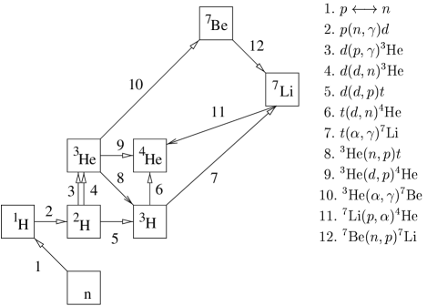
FIG. 1.: The reaction network that determines yields in standard BBN.

The new state of affairs (with corresponding advances in He and Li observations) has been described as a “precision era” for big-bang nucleosynthesis [5]. However, as the observational uncertainties shrink, the uncertainties on the calculated abundances begin to dominate. Although the nucleosynthesis calculation itself is straightforward, and has been well-understood for over three decades now [6, 7, 8, 9, 10, 11], “theoretical” uncertainties arise from its nuclear cross section inputs. These inputs consist of cross sections (Fig. 1) which have been measured in nuclear laboratories since the 1930’s, with accurate enough data for nucleosynthesis work dating mostly from the 1950’s and 1960’s. It is well-known that stellar nucleosynthesis requires cross sections below the Coulomb barrier, which cannot be directly probed in the laboratory because the cross sections are too small. In contrast, BBN occurs at sufficiently high temperatures ($T\sim 10^{9}$ K) that this is not a serious problem, and data are generally present at exactly the energies where they are needed for a BBN abundance calculation without any recourse to theoretical modeling. In fact, there is a sufficiently large body of precise data in the energy range needed for BBN that the results of the calculation have remained nearly the same since the standard code was first run by Wagoner in 1967 [6], despite a slow trickle of new cross section measurements. Nonetheless, some uncertainty remains in the calculations, arising from experimental uncertainties in determining these cross sections. These uncertainties range from about 5% to 25% in the cross sections, and propagate to errors of up to nearly a factor of two (from lower to upper $2\sigma$ limits) in the case of the calculated ⁷Li abundance. (This is true of “standard BBN,” which contains nothing beyond the standard model of particle physics. There are, of course, greater uncertainties if alternative – e.g. baryon-inhomogeneous – scenarios are considered [12, 13].)

The present “industry-standard” error estimation for the inputs was done by Smith, Kawano, and Malaney (hereafter SKM, Ref. [11]) in 1993, using the Monte Carlo error propagation method applied earlier by Krauss and Romanelli [10]. This was a landmark work because it examined all the nuclear inputs critically and in detail, and it placed quantitative error estimates on all the inputs. There has been a small number of new cross section measurements since [14, 15, 16, 17], which have been unevenly incorporated in subsequent work. Subsequent authors have continued to use the SKM rates and errors for most or all reactions. A few have substituted the results of a single new measurement in place of the corresponding SKM evaluation of all experiments for the given reaction.

Because the SKM uncertainties are used so widely to draw quantitative conclusions concerning many aspects of cosmology and particle physics, it is important to examine their assumptions and attempt improvement as well as to maintain some up-to-date set of uncertainties. The SKM work proceeds as follows: Cross section data for the key reactions (Fig. 1) are gathered from an extensive survey of the literature. These data are fitted to standard, if very approximate, theoretical expectations concerning their energy dependence (typically a low-order polynomial, for the low-energy $S$-factor), which has been widely used in previous work [18, 19, 20, 21]. Some arbitrary choices are made concerning inclusion and exclusion of data points in the fits, with a view to making these fits accurate over the energy range critical for BBN. Error estimation begins with formal error estimates on the fitted parameters, but is modified where necessary to include most or all data points within two-sigma error curves. This conservative approach justifies some arbitrariness in weighting the data sets. The SKM errors on the cross sections are summarized (with two exceptions) as uncertainties in the overall normalization, and then propagated through the basic BBN calculation by a Monte Carlo procedure with normalization values drawn from Gaussian distributions.

We begin by listing principles for a better treatment of nuclear data in a BBN calculation, commensurate with the goals of ensuring that the confidence limits being quoted in cosmological work are meaningful, and of making a direct link to the nuclear measurements. Because the energy dependences of the cross sections are not in question in most cases, our main goal is to arrive at a suitable method of estimating errors in the BBN yields. The desirable qualities for such a method are are: 1) Nuclear data, and their published uncertainties, should be incorporated into the BBN calculation as directly as possible, so that errors in the calculation are directly linked to the nuclear data set, and the results of the BBN calculation reflect as few arbitrary choices as possible; 2) minimal assumptions concerning functional forms of cross sections (as functions of energy) should be used, where there are enough data to characterize these functional forms (almost all cases); 3) there should be accounting for correlated errors in the data, since they are ubiquitous; 4) the incorporation of future data with smaller formal errors into the inputs should reduce the uncertainty estimates in the calculation; and 5) the prescription should be no more conservative than necessary, given the precision with which abundances are now being measured. The procedure of SKM, outlined above, does reasonably well on point number 2. Point number 5 is something of a matter of taste (although there is a mismatch in levels of conservatism between SKM and the errors quoted by astronomers). However, the SKM procedure does not answer well to our other requirements. The subjective assignment of errors causes trouble on points 1, 3, and 4. In particular, the conservative SKM method is not re-applicable in a way that narrows error estimates as new data are incorporated in the data set, unless old data are thrown out, and so it does not satisfy point number 4. Poor performance on this point discourages the production of more precise measurements, because it is unclear how new data will affect error estimates on reaction rates.

To improve on the SKM work, we propose a new prescription for treating the nuclear data that uses the measured cross sections directly in the standard big-bang nucleosynthesis calculation. It is a Monte Carlo technique that uses “realizations” of the full nuclear data set for the key reactions identified by SKM and Krauss and Romanelli to derive reaction rates. We extract final nucleosynthesis yields and confidence limits from distributions of yields corresponding to the distributions of cross sections implied in quoted experimental errors. While there may be some question of uniqueness, our method does provide a useful and unambiguous prescription for linking the results of the BBN calculation to its nuclear inputs. This method is very much in accord with the stated goals of earlier work, both of SKM and of Krauss and Romanelli [10], and it reflects increasing computer speed. In the words of Krauss and Romanelli, “unless error estimates are tied to a direct analysis of the data one cannot accurately gauge the margin for improvement.”

The rest of this paper is organized as follows: In Section II, we describe our Monte Carlo method for computing light-element yields and confidence intervals from the nuclear data. In Section III, we discuss the nuclear inputs in detail, emphasizing differences from the analysis of SKM. In Section IV, we discuss the results of a standard BBN calculation using our method. In Section V, we discuss the implications of our work both for the BBN calculation and for cosmology in general.

II method

For our purposes, the nuclear inputs for a BBN calculation come in the form of angle-integrated cross sections, $\sigma(E)$, where $E$ is reaction energy, reported in the published literature. The quantities needed to evolve abundances in a reaction network are thermally-averaged cross sections,

$$\langle\sigma v\rangle=\sqrt{8\over{\pi\mu(kT)^{3}}}\int\sigma(E)\,E\,e^{-E/kT}dE,$$ (1)

where $\mu$ is the reduced mass and $k$ is Boltzmann’s constant.

In the case of charged particles, the procedure typically followed in the past to obtain these thermally-averaged rates has been as follows: One first re-parameterizes the measured cross sections as $S$-factors,

$$S(E)=E\sigma(E)e^{2\pi\zeta},$$ (2)

where $\zeta=Z_{1}Z_{2}\alpha/v$, to remove the strong Coulomb dependence of the cross section. Here, $\alpha$ is the fine structure constant, $Z_{i}$ are atomic numbers of the nuclei, and $v$ is their relative velocity. The resulting function is then fitted to a low-order polynomial plus resonant terms to obtain a form which can be integrated. (This functional form has sometimes been used for extrapolation to low energy, although that is discouraged.) The integration of the nonresonant rate is then performed using a saddle-point approximation with lowest-order corrections [18, 19], or else performed numerically and fitted to the functional form one gets from the saddle-point integration. (The same considerations apply for neutron-induced cross sections, with the exception that they are fitted by a low-order polynomial in velocity before integration, and the integrations are then exact.) Resonant cross sections are fitted to Breit-Wigner or single-level $R$-matrix forms, integrated numerically, and fitted to analytic forms. While these functional forms are useful for disseminating evaluated reaction rates in printed form, and have therefore become somewhat standard, they are not ideal for producing rates valid over a wide range of temperatures or for arbitrary $S(E)$.

Both SKM and Krauss and Romanelli used this sort of procedure, including most of the extant data in the fits, and being careful that the fits were performed over the energy range needed for BBN calculations. They followed it up by estimating uncertainties on the reaction rates, expressed as errors in overall normalization (except for two cases of energy-dependent errors in SKM), which are appropriate to the BBN energy range. They then estimated the corresponding uncertainties in BBN yields by varying the rates according to these error estimates in Monte Carlo BBN yield calculations and examining the distribution of output abundances. The Monte Carlo approach was originally deemed necessary because it is not clear without doing the calculation whether the errors combine linearly. The recent work of Fiorentini et al. [22] indicates that in fact normalization errors on the reaction rates can be propagated linearly through the BBN calculation, and the results are very close to the corresponding Monte Carlo results.

Our method differs from that of these earlier efforts in several ways: we fold the process of characterizing reaction rates into the same Monte Carlo process that calculates abundances, we try to make the least possible number of assumptions about the functional forms of cross-section energy dependences, and we try to keep error estimation based strictly on quoted errors in the nuclear data set, including correlated errors explicitly.

Our Monte Carlo calculations sampled the space of nuclear cross sections indicated by the nuclear data, and the result was a distribution of output abundances, from which we derived confidence limits. Each calculation sampled 25,000 points in this space. (This was a number that gave us smooth 95% cl curves as a function of baryon density.) A single Monte Carlo sample consisted of the following steps:

1. For every measured cross section of every reaction (every $\sigma(E)$ in our database), a random number was drawn from a Gaussian distribution whose mean is the reported cross section at that energy, and whose variance is the reported variance for that point. Also, for each data set (collections of $\sigma(E)$ values from a given experiment), a random number was drawn from a Gaussian distribution whose variance was the normalization error shared by those points, and all cross sections in that data set were multiplied by this random normalization. This provided accounting for correlated errors. The database of cross sections and uncertainties is described in Sec. III below.

2. After “synthetic” cross section data were chosen, smooth representations of these data were created for integration. Specifically, the $S(E)$ (or $\sigma v$, for neutron-induced processes) curve for each reaction was fitted to a piecewise polynomial (in $B$-spline representation) as a function of energy. The spline broke up the energy axis into several (typically less than ten) segments, generally evenly-spaced in $\log E$, assumed a polynomial of order 3–5 within each segment, and forced continuity of derivatives across the segment boundaries. This curve was fitted to the simulated data by the customary weighted linear least-squares technique. Note that this approach is “theory-free” in the sense that the only assumption we have made about the cross sections is that they are sufficiently smooth functions of energy to be represented by the chosen piecewise polynomial. The $S$ factor re-parameterization is only a re-parameterization, and is converted back to cross sections after splines are fitted. Although the number of variables for our smooth representation was chosen by eye for each reaction individually, we expect that small variations in the functional form of the $S$ factor which depend on choices made in the fitting are smoothed out by the subsequent thermal averaging and Monte Carlo sampling.

3. The smooth representation of each cross section was integrated numerically at many different temperatures (ten per decade), and the resulting reaction rates fitted to a smooth representation as a function of temperature. This allowed subsequent calculation of rates by interpolation without expensive integrations.

4. Finally, these reaction rates were fed into a standard BBN code [8, 9], which used them to calculate yields. Note that since independent integrations of different numbers are performed for each Monte Carlo step, any (non-systematic) integration errors are accounted for in the Monte Carlo process.

When the code was finished, we extracted 95% confidence limits from the distribution of yields. This process is similar to a treatment of fitting errors described in Numerical Recipes [23].

We treated three reactions somewhat differently from the rest. First, we used the most recent experimental value for the neutron lifetime, $885.4\pm 2$ s, to derive values for the neutron-proton interconversion rates, choosing Monte Carlo values for this rate according to a Gaussian distribution with this mean and variance. These rates affect only the final ⁴He abundance significantly. This is also the only process ⁴He yields are sensitive to at likely values of baryon density. Lopez and Turner [24] have incorporated in a coherent and consistent way a number of small but important physics and numerical corrections to the weak rates, and we take yields for this nuclide from their work. Second, there was not enough data coverage to use our technique for proton-neutron capture, $p(n,\gamma)d$, so we used a theoretical model of this process as described in Sec. III D 1 below. Finally, the apparent presence of systematic discrepancies in measurements of the ${}^{3}{\rm He}(\alpha,\gamma)^{7}{\rm Be}$ cross section required the special treatment described in Sec. III D 8, after applying our standard technique to a subset of the data.

III nuclear inputs

A The Database

The nuclear data used in our work were obtained from a comprehensive survey of the experimental literature from approximately 1945 onward. Many of the numerical values were obtained from the on-line CSISRS database [25]. However, even in these cases, we incorporated data sets only after reading the original sources carefully. For almost all reactions, the data sets included were the same ones found in SKM. There are three reactions, $d(p,\gamma)^{3}{\rm He}$, ${}^{3}{\rm He}(n,p)^{3}{\rm H}$, and $t(\alpha,\gamma)^{7}{\rm Li}$, for which more recent cross section data than those used by SKM exist. Some subsequent BBN calculations (e.g., Ref. [1]) have incorporated the latest measurement of $t(\alpha,\gamma)^{7}{\rm Li}$ [14] by replacing the SKM fit with a reaction rate and uncertainty based on that measurement alone. These numbers have not found their way into all subsequent work (e.g., Ref. [22]), and we know of no calculations that have incorporated either of the recent TUNL measurements of the $d(p,\gamma)^{3}{\rm He}$ [15, 16] cross section (save one reported in this last experimental reference). One of our goals is to provide a new standard calculation which incorporates these measurements so that they are not ignored in future theoretical work.

Another of our major goals is to incorporate explicitly information concerning known systematic errors in the cross section measurements, which indicate correlations among data from a given experiment. The incorporation of this information into our Monte Carlo calculation is described in Sec. II above. Here, we describe the origin of the numbers used. Data sets which include measurements of the cross section for the same process at several energies contain both shared normalization errors (which affect all points in that data set) and unshared point-to-point errors (which vary from one point to the next, and arise primarily from counting statistics). Because it is generally much more difficult to determine the absolute normalization of a cross section than it is to measure its energy dependence, most of the uncertainty in a given cross section is usually in its normalization. It is therefore important to treat normalization errors in the data properly when combining data sets, especially if the data sets are of different sizes. It is not correct to apply the quoted “total error” for each point in a fit when the correlated errors have been added in (the usual case for published data). Our calculation assumes Gaussian-distributed errors as the simplest assumption in every case, although one might expect that normalization errors, in particular, will not be Gaussian-distributed. Note that in other contexts, one typically allows a floating overall normalization for each data set in fitting nuclear data. Since the energy dependences are well-determined for almost all of the eleven key cross sections, we are only interested in experiments which measure the cross section normalization.

Separate treatment of shared and unshared errors involves some difficulties. These include the fact that systematic effects may not be well-quantified, and the fact that experimental data have often been presented in ways incompatible with this goal. Several of the experimental sources (especially the more recent ones) explicitly state shared normalization errors separately from unshared errors. In some cases, quoted normalization errors had to be subtracted from quoted total errors, which are quadrature sums with unshared errors. Other experimental sources did not explicitly add up the shared errors, but they usually listed the percent contribution from each major item in the error budget separately. These could usually be added up to provide normalization errors, with a small amount of guesswork as to which contributions to place in each category. For example, detector efficiencies and target chemistry are often readily identifiable as sources of shared error, in those cases where they are. Because errors are almost always added in quadrature, our procedure was not strongly dependent on identifying which category (shared or unshared) each individual contribution should be placed in, so long as we were careful that estimates of unshared errors did not become too small. We are confident that the sizes of errors adopted for our database are all roughly correct. Our method required that we exclude a small number of data sets which did not provide enough information for such a breakdown of error sources (but we were biased toward keeping data sets, especially where there were few measurements of a cross section). We also excluded data sets which only represent measurements of relative cross sections. Fortunately, we did not need to exclude a large number of data sets for any reason.

We have not incorporated any of the substantial body of theoretical knowledge (ranging from unitarity constraints to “microscopic” reaction models) which exists for some of these processes into the database, except for the process $p(n,\gamma)d$. The reason for this is that there is little need for theoretical evaluations where we already have large amounts of data, especially since errors are often hard to assign to models. A typical use of theoretical models is to calculate an energy dependence for a cross section, test it by comparison with relative cross section measurements, and then normalize it by absolute cross section measurements. This is more constraining than our approach, since it allows data taken at all energy ranges (and sometimes in other reaction and scattering channels) to affect the evaluated cross section at a given energy, but it would require a significantly larger and less straightforward effort. In this regard, our “theory-free” approach may still provide conservative error estimates for some reactions.

Because of all these concerns, particularly those concerning unknown systematics and arbitrariness of error assignment in experiments, there can probably be no unique evaluation of rates and their errors. We have attempted to make estimates with the desirable qualities listed above, and to improve on previous efforts.

B Reaction Sensitivities

Because our approach to the BBN calculation is very closely tied to the data, we are able to make very precise statements about exactly which inputs the calculated yields are sensitive to (at least for the “standard BBN” calculation we have done). In particular, we have quantified this sensitivity with what we call “sensitivity functions” for each reaction and nuclide. These may be regarded as functional derivatives of BBN yields with respect to reaction $S$ factors. For a given reaction and nuclide, we calculate one of these functions numerically by adding a small amount to the reaction $S$ factor over a narrow bin in energy, and computing the resulting primordial abundance of that nuclide. The sensitivity function is the fractional difference between this yield and the unperturbed yield, as a function of the location of the energy bin. In the limit of very narrow energy bins, this is a functional derivative. The functions indicate quantitatively the exact energies at which each process is important in standard BBN, and therefore the exact energies at which precise cross section measurements are needed to produce precise BBN calculations. We denote the sensitivity functions by $g_{2}(E)$ for D/H and $g_{7}(E)$ for ⁷Li/H, and they are shown for all eleven cross sections below.

The general behavior of these functions is clear: Above some temperature in the vicinity of $10^{9}$ K, the actual reaction rates do not matter because the reactions are in thermal equilibrium, with forward and reverse reactions proceeding at the same rate. When the density and temperature drop to some point at which a particular reaction falls out of equilibrium, its rate may become a determinant of the nuclide abundances. Finally, there comes a point when temperatures and densities are too low for a reaction to change abundances at all. The approximate effective energies of reactions for nuclear burning at a given temperature correspond to the customary “Gamow peak” of nuclear astrophysics [18], and what we see in the sensitivity function is often the Gamow peak, convolved with the distribution of temperatures at which a given reaction is active, but out of equilibrium. The rate sensitivities are also functions of the baryon density, as indicated in the plots of Sec. III D.

C Statistical tests

Our new method for calculating BBN abundances should be examined to test the robustness of its results and the consistency of the input nuclear data. We therefore applied it to fake data drawn from the assumed source distribution of the actual data. We generated (for each reaction) fake data that were Gaussian-distributed about our highest-probability curve. Correlated data were multiplied by appropriate Gaussian-distributed common normalizations. The fake data were placed at the same energies as the actual data, and the distributions were based on the quoted errors of the corresponding actual data. For each collection of fake data, we applied our Monte Carlo curve-fitting method, and computed the means, $\mu(b_{i})$, and standard deviations, $\sigma(b_{i})$, of the $B$-spline coefficients describing the fitted curves. ($b_{i}$ denotes the coefficient of the $i$th basis function. Note that the local support of $B$-spline basis functions [26] makes each of these coefficients a sort of weighted local average of the fitted function, so that $\mu(b_{i})$ and $\sigma(b_{i})$ reflect the means and standard deviations of the fitted curves directly.) After performing this procedure for many ($\geq 1000$) collections of fake data, we computed the means, $\overline{\mu(b_{i})}$, $\overline{\sigma(b_{i})}$ and standard deviations $\Sigma(\mu(b_{i}))$, $\Sigma(\sigma(b_{i}))$ over the fake-data distribution of the $B$-spline coefficient means $\mu(b_{i})$ and standard deviations $\sigma(b_{i})$ derived from each choice of fake data.

Comparison of these numbers with the means and variances of $B$-spline coefficients generated as intermediate numbers by our BBN code indicates that the means reproduce the assumed curves consistently with our error estimates in all but one case. The mean variances $\overline{\sigma(b_{i})}$ of the $B$-spline coefficients generally agree with the standard deviations of $B$-spline coefficients from our BBN procedure (which are $\sigma_{i}$ for the actual data); where they differ, our BBN procedure gives slightly larger standard deviations. The standard deviations of the means, $\Sigma(\mu(b_{i}))$, were virtually always identical to the mean standard deviations, $\overline{\sigma(b_{i})}$. In other words, the distributions of $S$-factor curves from our procedure do not change drastically when the experimental data are drawn from other points in the same distributions from which we assume the actual data to be drawn. Serious errors in reproducing the assumed curves occurred only for ${}^{3}{\rm He}(d,p)^{4}{\rm He}$.

We repeated the same numerical experiment, this time simulating a factor-of-two underestimation of all normalization errors by adding extra scatter to the fake data (doubling all of the normalization errors). In applying our Monte Carlo method to these fake data, we assumed the quoted normalization errors, not the inflated ones. The most noticeable results were an increase in the standard deviations of means $\Sigma(\mu(b_{i}))$ by a factor of about $\sqrt{2}$, and slighly poorer reconstruction of several coefficients for $t(\alpha,\gamma)^{7}{\rm Li}$. Very little else changed. The standard deviations over fake data of the $B$-spline variances, $\Sigma(\sigma(b_{i}))$, also increased in some cases, but were seldom much more than 10% of $\overline{\sigma(b_{i})}$. In other words, the variances of the $S$-factor curves from our BBN procedure are sensitive mainly to the error estimates rather than the quoted cross sections, while the mean curves are less sensitive to the error estimates. Underestimated errors result in $S$-factor curves that vary less than they should in our BBN calculation, but probably never by factors of more than 1.5.

Although the results above suggest that our method is not overly sensitive to unexpected scatter in the data, we still wish to address the question of consistency of the nuclear data. We calculate a chi-squared statistic with the data and the “best-fit” model curve describing the un-altered data. This is not a goodness-of-fit test for our modelling, because the individual curve plays no important role in our calculation. It is, rather, a benchmark by which to examine the consistency of data measured at different energies. Initially, we calculated this chi-squared statistic using the full non-diagonal error matrix, as described in Ref. [27]. However, as this reference shows, chi-squared calculations using the non-diagonal error matrix are not appropriate when the correlations are in the form of shared normalizations. Fits minimizing this statistic are almost always lower than the data when there are large normalization errors.

The statistic that we did apply is the ordinary $\chi^{2}$ statistic, defined as

$$\chi^{2}=\sum_{i}\frac{(S(E_{i})-S_{\rm model}(E_{i}))^{2}}{\sigma_{i}^{2}},$$ (3)

where $S(E_{i})$ are the data for a given reaction, measured at energies $E_{i}$, $S_{\rm model}(E)$ is the best-fit model curve, $\sigma_{i}$ is the quadrature sum of normalization and point-to-point errors for each datum, and the sum is over all data for a given reaction. Because of the correlated errors, we do not expect this statistic to be distributed as a formal chi-squared distribution. We therefore constructed the expected distribution by varying fake data about the best-fit curve according to the quoted uncertainties as above. This allowed us to assess consistency of the data by determining the likelihood of the actual value of $\chi^{2}$, given our assumptions about the distribution from which the actual data were drawn. The results of computing $\chi^{2}$ for each reaction $S$-factor and comparing it to the fake data distribution are shown in Table I. From these results, we conclude that the only clear case of trouble is ${}^{3}{\rm He}(d,p)^{4}{\rm He}$. Note that this cross section has no noticeble effect on the calculated deuterium abundance, and very little effect on the calculated ⁷Li abundance. It is more important for ³He, which is not as yet amenable to high-precision treatment as a product of BBN.

The reader may object that we do not have a procedure to inflate the errors where the $\chi^{2}$ test indicates that they may have been underestimated, or to discard data sets which contribute disproportionately to $\chi^{2}$. We have resisted adopting such procedures for several reasons. The first is that it would be difficult to arrive at a unique and meaningful prescription to determine by how much to inflate errors, or which data to discard. (The customary multiplication by the square root of the $\chi^{2}$ per degree of freedom is not suitable because $\chi^{2}$ is not distributed as a formal $\chi^{2}$ distribution, and because the factor should in principle be a function of energy.) The second reason is that we would like to leave any systematic problems with the existing data, and their properties with regard to generating formal errors for BBN, as distinct issues. A database which performs well on both counts is desirable for producing reliable BBN calculations. On the other hand, discarding data is something we will not do without good reasons from the nuclear physics literature, even though disproportionately large fractions of the $\chi^{2}$ statistics usually do come from individual data sets in our database. Finally, there is only one “two-sigma” unlikely $\chi^{2}$ in Table I, although there are more “one-sigma” unlikely values of $\chi^{2}$ than expected.

TABLE I.: For each reaction, the number of data points, characteristics of the piecewise polynomial descriptions, values of $\chi^{2}$, and probabilities that $\chi^{2}$ exceeds its measured values (based on 20,000 Monte Carlo samples).

		Spline			${Probability}$
Reaction	Points	segments	order	$\chi^{2}$	$ofexceeding\chi^{2}$
p(n,$\gamma$)d	—	1	10	(not fitted to lab data)
d(p,$\gamma$)3Hea	16	5	3	$3.40$	$93\%$
d(d,p)3H	134	6	3	$108.0$	$68.7\%$
d(d,n)3He	130	6	3	$106.7$	$64\%$
3He($\alpha$,$\gamma$)7Beb	118	4	3	$138.3$	$37\%$
3He(d,p)4He	111	9	4	$315.0$	$0.5\%$
3He(n,p)3H	240	5	5	$106.0$	$91\%$
7Li(p,$\alpha$)4He	105	6	3	$193.1$	$11\%$
7Li(p,n)7Be	137	29	3	$223.0$	$16\%$
3H($\alpha$,$\gamma$)7Li	55	6	3	$129.5$	$12\%$
3H(d,n)4He	213	15	3	$292.8$	$13\%$

D Individual Reactions

The following section is dedicated to detailed discussions of the data sets for each individual reaction. For convenience, we have followed the same ordering as SKM in discussing individual reactions. Because the available data have changed very little since the work of SKM, we emphasize differences from their analysis and new insights provided by our examination of the inputs. We also list the references from which we compiled our database. Unless explicitly discussed, any omission was because either a normalization error could not be extracted from the original source, or the experiment measured only relative cross sections (or, trivially, the experiment contained no data in the relevant energy range).

For each reaction, we show in a graph (Figs. 2–12) the input data, the “best-fit” curves and 95% confidence limits inferred from our Monte Carlo procedure (solid curves), and (where available) the corresponding curves from the SKM analysis (dash-dotted curves), and curves from the ENDF-B/VI [28] evaluation (dashed curves). The tick marks below the data in each graph show the region over which the integral must be performed to get the yields correct to one-tenth of the total uncertainty in all abundances (inner tick marks), and to get the yields correct to one part in $10^{5}$ (outer tick marks).

In the lower panels of each graph, we show the sensitivity functions at baryon densities of $\Omega_{B}h^{2}=0.019$ (solid curves) and $\Omega_{B}h^{2}=0.009$ (dashed curves) for D and ⁷Li. They represent very well the contribution of the $S$ factor uncertainties to the final yield uncertainties as functions of reaction energy in the sense that, to a good approximation, the convolutions of these curves with the 95% cross section limits gives the 95% yield limits due to that reaction indicated by the Monte Carlo study described below. The $g$ functions shown in the plots have been multiplied by energy in MeV so that relative areas under the curves can be accurately judged on the logarithmic scale on which we have plotted the nuclear data. Some references contained two or more distinct data sets with different normalization errors; in these cases, an extra number after publication year distinguishes symbols from the same publication. All energies are in the center-of-mass frame.

1 $p(n,\gamma)d$

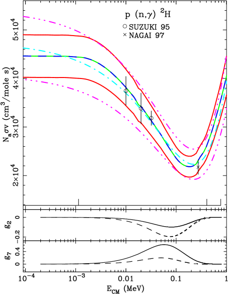
FIG. 2.: Theoretical curve from Hale et al. [29], SKM fit to that curve with $2\sigma$ errors, and current experimental data in the BBN energy range [30, 31]. An explanation of our nuclear data figures may be found near the beginning of Sec. III D.

As noted above, this reaction required special treatment. It could not be subjected to our piecewise splining or Monte Carlo sampling of data points because of an extreme scarcity of data in the $E_{CM}<300$ keV range. This is despite recent efforts to measure this crucial cross section [30, 31] in the relevant energy range, which have so far resulted in only four data points. We have chosen as the cross section for this process its evaluation in the ENDF-B/VI database [29]. This cross section derives from a theoretical model computed sometime around 1970, constrained by $np$ scattering phase shifts, along with a few photodisintegration data (known to have systematic problems), and it has seen a minor update to match the current value of the well-measured thermal-neutron capture cross section [32]. No documentation for this model survives. The crucial energy range for BBN corresponds to a changeover in reaction mechanisms (from $M1$ capture to $E1$ capture) for this process, so one might expect the validity of the evaluation to be most in question there. It has held up remarkably well in light of the recent measurements, but its authors view this as a fortuitous coincidence [33]. SKM estimated a 5% uncertainty on this evaluation, based on uncertainties quoted in earlier tabulations of the cross section for practical use. It is very difficult to trace the origin of this number, but we have adopted a 5% Gaussian-distributed normalization error as the uncertainty in this cross section — both for consistency with SKM, and because it is not too far from an estimate by the evaluation’s authors of “at least 10%” [33]. (Note that the 7% total uncertainty quoted by SKM includes errors in further fitting and integration. We do no further fitting, and we estimate an error of less than 1% in our numerical rate integrations.)

2 $d(p,\gamma)^{3}{\rm He}$

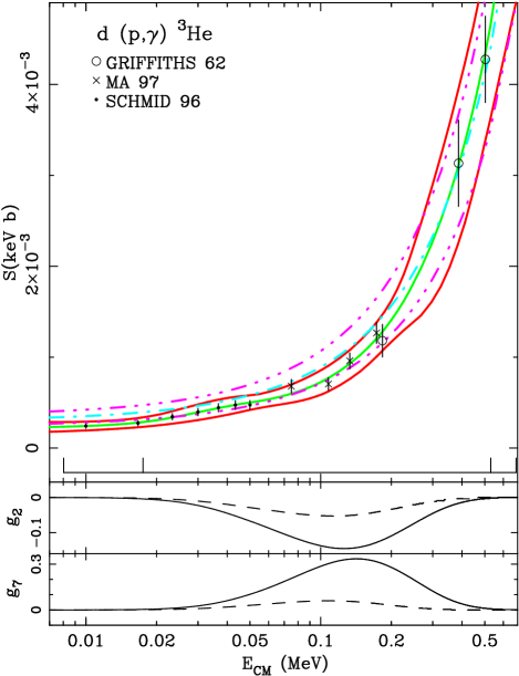
FIG. 3.: $S$ factor data and fits for $d(p,\gamma)^{3}{\rm He}$.

The data set for this reaction is not well suited to our method. Of the three experiments performed before 1990, the experiment of Bailey et al. [34] is only a relative measurement, and not suited to our method; the low-energy experiment of Griffiths et al. [35] deconvolved thick-target data with a simple model of combined $S$- and $P$-wave capture at a sharp nuclear surface. The resulting energy dependence is in conflict with both the more recent measurements of Schmid et al. [15] and the three-body microscopic calculation of Viviani et al. [36]. The recent TUNL experiments [15, 16] also suggest that these earlier thick ice target experiments used the wrong stopping powers, resulting in cross sections about 15% too high. We excluded the Griffiths et al. and Bailey et al. data sets for these reasons, but only after checking that their omission did not alter our results drastically. As indicated below, this reaction contributes a large portion of our uncertainty estimates. The only other experiment in our database for this reaction is from Ref. [37].

The sparseness of the data may be a cause for concern regarding our treatment of this cross section. However, it is encouraging that our splines indicate much the same energy dependence as the microscopic calculation [36, 16], so the sparseness is probably not such a big problem. Our errors reflect the $\sim 8\%$ normalization errors in the best measurements of the cross section.

3 $d(d,n)^{3}{\rm He}$

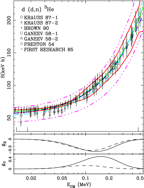
FIG. 4.: $S$ factor data and fits for $d(d,n)^{3}{\rm He}$.

The deuteron-deuteron reactions have been measured very extensively for fusion applications, and they are especially well-constrained below about 60 keV by the precise measurements of Brown and Jarmie [38]. The SKM errors were based on an apparent discrepancy between these data and those of Krauss et al. [39]. Brown and Jarmie make a similar assessment of the situation, and recommend renormalizing the Krauss et al. data to their more precise data (which we do not do). It is important to note that most of the error in both cases is contained in normalizations, so the case is not a 10% discrepancy between ten data points with $8\%$ errors and eleven points with 1.5% errors. Note that the sensitivity functions peak at 100 keV or above, beyond the Brown and Jarmie data. With the exception of Krauss et al. (with an $8\%$ claimed normalization error), all of the data in this region date from before 1960, and their large errors and scatter are responsible for the large contribution of this reaction to the uncertainties in BBN yields. Other data for this reaction are from Refs. [40, 41, 42].

4 $d(d,p)t$

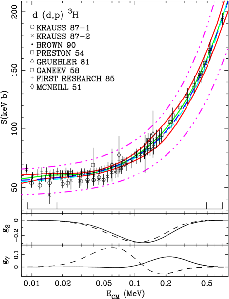
FIG. 5.: $S$ factor data and fits for $d(d,p)t$.

This cross section is generally measured concurrently with that of $d(d,n)^{3}{\rm He}$, so most of the discussion for that reaction carries over to this one. The sensitivity functions here are more complicated, but there is still a large contribution at energies greater than 100 keV. There are also fewer data above 100 keV in this case, reflecting the use of neutron-specific detection methods in some $d(d,n)^{3}{\rm He}$ experiments. Again, few of the data which are present in this range come from modern experiments. The data for this reaction were taken from Refs. [38, 39, 40, 41, 42, 43, 44].

5 ${}^{3}{\rm He}(n,p)t$

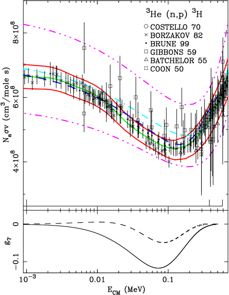
FIG. 6.: $S$ factor data and fits for ${}^{3}{\rm He}(n,p)t$.

The data set for this reaction consists of cross sections for both the forward (Refs. [45, 46, 47, 48]) and reverse (Ref. [17, 49]) processes. We used reverse data that had been converted to forward cross sections through exact detailed balance relations, along with direct data. The SKM fit included numbers from Alfimenkov [50], which we did not obtain, but the important difference between our analysis and that of SKM is that they excluded the very precise measurement of Borzakov et al. [45], which owes its small quoted uncertainty to a normalization from ${}^{6}{\rm Li}(n,\alpha)^{3}{\rm He}$ data intended for metrological use [51, 52]. SKM excluded this data set because it decreases with energy more quickly than the other data, ending lower than any of them at 100 keV. This, combined with the small quoted errors, would have forced their second-order polynomial fit below the data at higher energies. However, this is not a problem for our piecewise spline approach, which decouples errors arising from different experiments at different energies. The extensive and much-needed data which Brune et al. [17] published recently for this cross section also agree more closely with the Borzakov et al. than with SKM.

6 $t(d,n)^{4}{\rm He}$

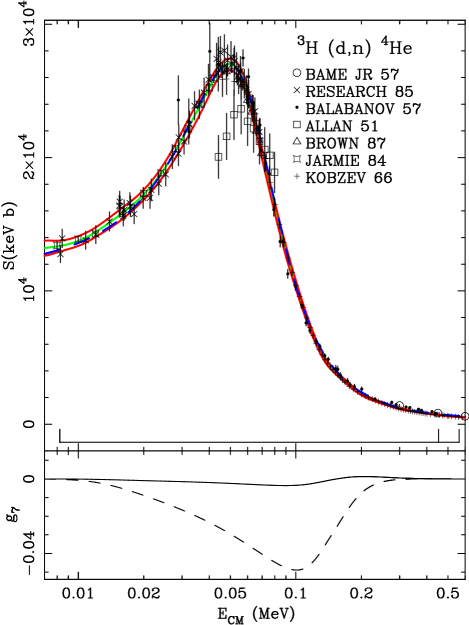
FIG. 7.: $S$ factor data and fits for $t(d,n)^{4}{\rm He}$.

The definitive measurement of the cross section for this process, up to 70 keV, is by the Los Alamos group [53, 54], and it has a quoted normalization error of 1.4%. Other measurements in our database come from Refs. [42, 55, 56, 57, 58]. As SKM point out, there are no modern experiments on the high-energy side of the resonance. However, this reaction does not contribute noticeably to the uncertainty in D or ⁷Li yields.

7 ${}^{3}{\rm He}(d,p)^{4}{\rm He}$

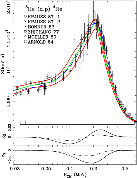
FIG. 8.: $S$ factor data and fits for ${}^{3}{\rm He}(d,p)^{4}{\rm He}$.

There is considerable scatter in the data for this process, as reflected in the very low probability of the $\chi^{2}$ statistic. In the case of the Bonner et al. measurement [59], this may be attributable to energy straggling in the gas target’s Al window. In any case, there is little else to say here except to point out that our piecewise spline seems to represent the data about as well as the SKM $R$-matrix fit. This reaction contributes a large portion of the uncertainty in the ³He yield. Other data used for this reaction are from Refs. [39] and [60, 61, 62]. The low-energy data of Schröder et al. [63], intended to probe electron screening, were omitted here because they did not measure the absolute cross section.

8 ${}^{3}{\rm He}(\alpha,\gamma)^{7}{\rm Be}$

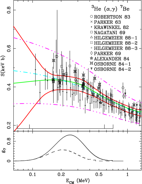
FIG. 9.: $S$-factor data and fits for ${}^{3}{\rm He}(\alpha,\gamma)^{7}{\rm Be}$. Note that the data of Kräwinkel et al. [64] have been renormalized as suggested by Hilgemeier et al. [65].

The apparent discrepancy at $2\sigma$ between experiments that observe capture gamma rays from this process (Refs. [64, 65, 66, 67, 68, 69]) and those that observe photons from the ⁷Be decay (Refs.[69, 70, 71]) is well-known from discussions of the solar neutrino problem [72]. Our direct approach to the data makes no use of the (well-understood) theory of this process, and the activation technique has only been used at energies too high to affect big-bang nucleosynthesis (although the Volk et al. [71] results are quoted as extrapolated $S(0)$ values only). However, the energy dependence of this reaction is sufficiently well-determined from the capture photon experiments to justify the use of an “activation method” curve obtained by renormalizing the fit of the capture-photon-derived cross sections to match the activation points.

After the main run, we re-ran our Monte Carlo sampling, renormalizing the ${}^{3}{\rm He}(\alpha,\gamma)^{7}{\rm Be}$ cross section from the capture-photon measurements by the mean of the activation measurements, and drawing the renormalization from a Gaussian distribution based on the variance of the activation measurements. For this purpose, we use the reference of all cross sections to zero energy found in Adelberger et al. [72]. The effect of this discrepancy (amounting to a systematic shift of 13%) is easy to understand; all ⁷Li produced at high $\Omega_{B}$ comes from this reaction, so changes in its rate result directly in changes of the final ⁷Li yield. The result is a shift of 11% in our confidence limits for ⁷Li, a significant fraction of the widths of these limits, at high $\Omega_{B}$. (See below.) If the activation measurements are correct, this would exacerbate the problem of ⁷Li depletion in halo stars — a point which has not previously arisen in discussions of this problem because it represents a much smaller fraction of the widths of the SKM ⁷Li limits, and because SKM dropped the activation data from their evaluation altogether.

9 $t(\alpha,\gamma)^{7}{\rm Li}$

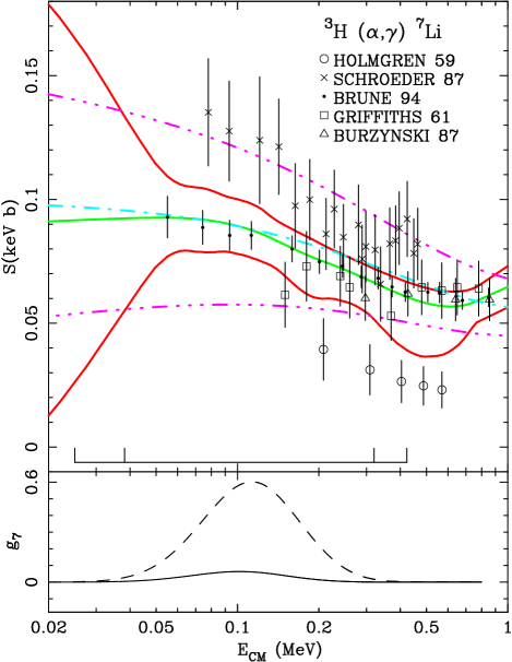
FIG. 10.: $S$ factor data and fits for $t(\alpha,\gamma)^{7}{\rm Li}$.

A precise new measurement of the cross section for this process has been completed by Brune et al. [14] in the time since the publication of SKM. Some subsequent calculations have incorporated the reaction rate derived from that measurement by its authors (e.g., Copi et al. [1]), using as the uncertainty the 6% uncertainty in the experiment’s cross section normalization. Krauss and Romanelli [10] pointed out that it is not always the best policy to base calculations on only the most recent measurement, and we agree. The previous data, Refs. [73, 74, 75, 76], do show a great deal of scatter, and our best-fit curve tends to follow the more-precise Brune et al. data, as it should. Relative to the SKM yields, this has little effect at high baryon density, but it decreases the ⁷Li yield slightly at very low baryon density, where this process makes most of the ⁷Li. We have omitted the Coulomb-breakup measurement of Utsunomiya et al. [77] because the Coulomb-breakup process is not completely understood for this reaction (as discussed in SKM) and because the cross section energy dependence derived from this method disagrees with the Brune et al. data. We note that the problem with normalization of the Schröder et al. [74] and Griffiths et al. [75] data sets mentioned by SKM seems to have gone away in the intervening time [78].

10 ${}^{7}{\rm Be}(n,p)^{7}{\rm Li}$

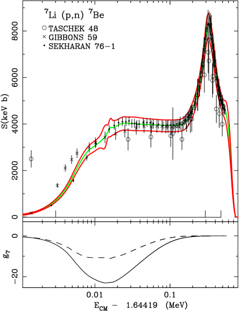
FIG. 11.: $S$ factor data and fits for ${}^{7}{\rm Li}(p,n)^{7}{\rm Be}$.

We fitted the cross section for the reverse of this process, since there are no direct data in the energy region of interest for BBN. This may not be the ideal choice, since the curve has a very large second derivative just above threshold. We fit data for ${}^{7}{\rm Li}(n,p)^{7}{\rm Be}$ from Sekharan et al. [79], Taschek and Hemmendinger [80], and Gibbons and Macklin [49], which extend from threshold to well past the lowest-energy resonance. We also cut off these data sets at about 700 keV above threshold (where they no longer affect BBN yields), so that only data in the critical range affect the $\chi^{2}$ calculations. Although this reaction contributes very little to our error budget (see Sec. IV below), it is important to recognize the scarcity of data and the lack of detailed error analysis in the original sources.

11 ${}^{7}{\rm Li}(p,\alpha)^{4}{\rm He}$

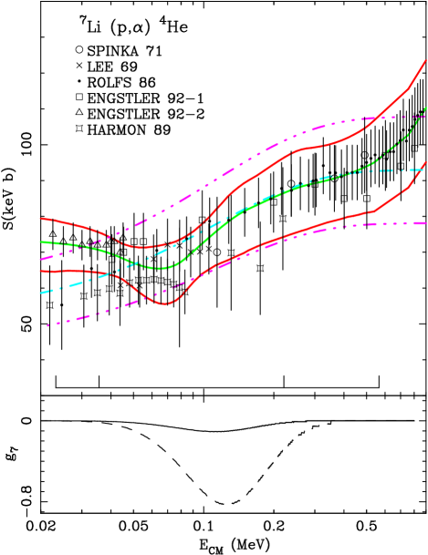
FIG. 12.: $S$-factor data and fits for ${}^{7}{\rm Li}(p,\alpha)^{4}{\rm He}$.

The low-energy cross section for this process is represented by a small number of measurements, Refs. [81, 82, 83, 84, 85], and is determined over most of the energy interval of interest to us by the data of Rolfs et al. [83]. We have kept the data of Engstler et al. [84] below 50 keV in our fit, even though the slight rise in this data set relative to that of Harmon [85] has been attributed to electron screening effects. (The data of Harmon were normalized to the ${}^{6}{\rm Li}(p,\alpha)^{3}{\rm He}$ cross section in such a way that they have been “corrected” for screening to some extent [84].) The fact that our $S$-factor curves follow the small error bars of the low-energy Engstler et al. data is not too distressing, since the sensitivity function for lithium production for this reaction is very small below 40 keV, and a true correction for screening would require a thorough theoretical treatment, e.g., $R$-matrix techniques with a direct reaction mechanism. It is not clear that simply extrapolating fits to simple functions from higher energies is valid, or that the data of Harmon et al. reflect a true correction for screening.

E Recommended Rates and Errors

A disadvantage of our method, relative to earlier efforts, is that it requires the whole nuclear database and a larger amount of computer time, as well as a significant modification of existing BBN code. Reaction rate uncertainties are also harder to quote than in the SKM prescription, since uncertainties at different temperatures are neither completely correlated nor completely uncorrelated. In any case, the rates produced by our code are not suitable for any use significantly different from the standard BBN calculation, and our method is specific to the BBN context, where only a few cross sections — well-represented at the right energies by available data — are needed. We note, in particular, that the “flaring” of our piecewise polynomial fits at high and low energy does not contain any physical information at all, but only the fact that polynomial interpolations always blow up beyond the limits of the data they were fitted to. For general use (especially outside the BBN energy region), we suggest using rates from a more general compilation, such as the NACRE compilation [86], intended to succeed the Caughlin and Fowler [21] charged-particle reaction rates.

IV results

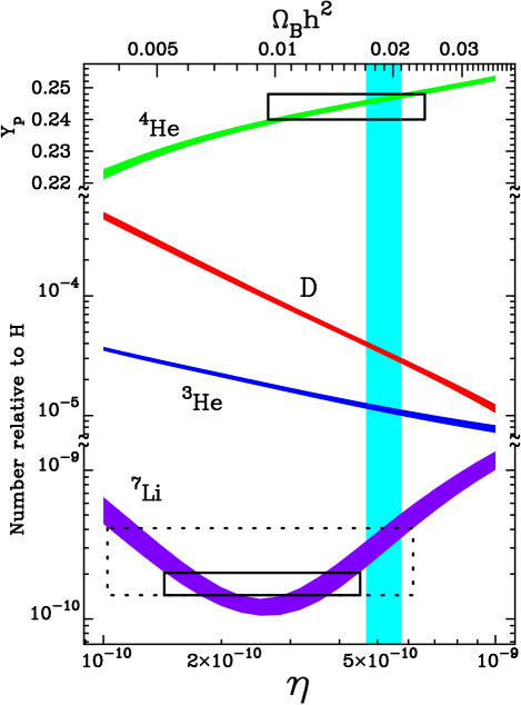
FIG. 13.: Summary of the 95% confidence intervals for the BBN predictions for D, ³He, ⁴He and ⁷Li. The ⁴He uncertainty comes from Ref. [24]. Boxes indicate 95% cl abundances from observation [87, 88, 89]. The vertical band indicates our 95% cl baryon density inferred from the Burles and Tytler  [2, 3] deuterium observations.

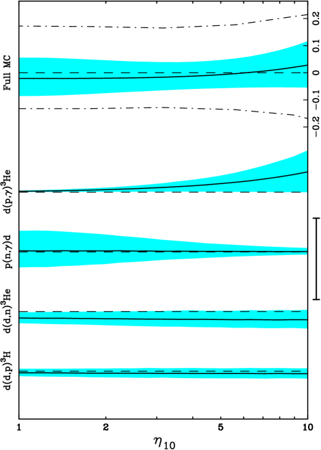
FIG. 14.: Fractional changes (solid curves) and revised 95% confidence limits (shaded regions) in D/H from our full Monte Carlo calculation and from Monte Carlo studies of individual reactions, relative to the SKM yields and errors (dashed lines). For comparison, the vertical bar at the side of the figure indicates the $1\sigma$ uncertainty in the Burles and Tytler D/H measurements [2]. All curves are on the same scale.

In discussing the results of applying our prescription, we concentrate on the predictions of ⁷Li and D yields. On the one hand, the observational status of ³He is not such as to motivate precise comparisons with the calculation. On the other, the errors in ⁴He, especially at higher values of $\Omega_{B}$, are dominated by the uncertainty in the weak coupling constant and by uncertainties in calculating the matrix elements for the weak processes. These errors and theoretical uncertainties have been analyzed exhaustively by Lopez and Turner [24], and we have not included all the apparatus of their treatment in our BBN code; we take their results for this nuclide to be definitive.

Our most important results, apparent from Figs. 13, 14, and 15, are reductions by factors of up to three in the width of the 95% confidence intervals for both the ⁷Li and D yields relative to SKM. The median values of our yields are almost identical to those obtained from the SKM rates, the difference being well within our estimated errors. These small changes can generally not be attributed to any one reaction, but to some nonlinear addition of changes from several reactions, as indicated in Fig. 15.

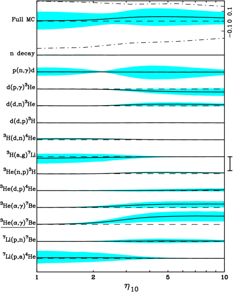
FIG. 15.: Changes (solid curves) and 95% confidence intervals (shaded regions) in $\log(^{7}{\rm Li/H})$ from our full Monte Carlo calculation and from Monte Carlo studies of individual reactions, relative to the SKM yields and errors (dashed lines). The vertical bar on the side indicates $1\sigma$ error in the Spite-plateau abundance [87]. The underlined reaction label indicates the individual-variation result using the alternate rate for ${}^{3}{\rm He}(\alpha,\gamma)^{7}{\rm Be}$, as described in the text. All curves are shown on the same scale.

We did not expect a huge change either in the size of the error estimates or in the calculated most-likely BBN yields. We did expect some reduction in the error estimate because we did not go out of our way to be conservative. The reduction in the size of our error estimates is largely a side-effect of our method of handling the nuclear data, chosen as a way of relating uncertainties in the calculated yields to uncertainties in the nuclear data.

We also studied the error contributions of individual reactions by setting all rates but one to their SKM values, and applying our Monte Carlo technique to that reaction alone. As shown in Figs. 14 and 15, this indicates the relative importance of each reaction as a function of baryon density (much as in the figures of Krauss and Romanelli [10]). This shows exactly which reaction rates need improvement to reduce the errors on BBN yields. In turn, the knowledge of which cross sections need improvement can be combined with the sensitivity functions of Sec. III and Figs. 2 through 12 to indicate the specific energies at which they need improvement. The “most wanted” for the deuterium abundance are, from most to least important at $\Omega_{B}h^{2}=0.019$: $d(d,n)^{3}{\rm He}$ above 100 keV; $d(p,\gamma)^{3}{\rm He}$ everywhere; $d(d,p)^{3}{\rm H}$ above 100 keV, and $p(n,\gamma)d$ at 30–200 keV. For ⁷Li, the leading contributions to the uncertainty at $\Omega_{B}h^{2}=0.019$ are from $p(n,\gamma)d$ at 20–150 keV, ${}^{3}{\rm He}(\alpha,\gamma)^{7}{\rm Be}$ at 150-375 keV (and overall normalization), $d(p,\gamma)^{3}{\rm He}$ everywhere, and $d(d,n)^{3}{\rm He}$ above 100 keV. At $\Omega_{B}h^{2}=0.009$, the uncertainty in ⁷Li comes mainly from ${}^{3}{\rm H}(\alpha,\gamma)^{7}{\rm Li}$ and ${}^{7}{\rm Li}(p,\alpha)^{4}{\rm He}$.

Taking this list one step further, we have generated fake data for some of these reactions (following the best-fit curve) and placed it in our database. In each case, fake data were placed on twenty evenly-spaced intervals between 5 and 500 keV center-of-mass. We then re-did the single-reaction Monte Carlo for that reaction, and reduced the size of the normalization error on the fake data set until the uncertainty estimate due to that reaction was reduced by half. The sizes of the normalization uncertainties required by this criterion are given in Table II. We assumed that unshared errors can be made arbitrarily small, and left them out. Similar fake data sets modeling proposed experiments could be used to determine what effect they would have on the BBN error estimates in our formalism.

TABLE II.: Size of normalization error necessary in a new data set (of twenty points evenly-spaced from 5 to 500 keV) for its addition to our database to reduce the single-reaction error estimate on the indicated BBN yields by half at $\Omega_{B}h^{2}=0.019$.

Reaction	$Desirederrorincrosssection$	BBN product
$d(p,\gamma)^{3}{\rm He}$	$3.2\%$	D
‘$d(d,n)^{3}{\rm He}$	$2.0\%$	D
$d(d,p)^{3}{\rm H}$	$1.6\%$	D
${}^{3}{\rm He}(\alpha,\gamma)^{7}{\rm Be}$	$2.3\%$	7Li

While the ³He chemical evolution and abundance measurements are too uncertain to motivate high-precision comparisons with the calculation [5, 90, 91, 92], we have also examined the results of our calculations for this nuclide and for its reaction-rate dependences. The results are indicated in Fig. 16. The slope of the dependence of this abundance on baryon density has changed relative to the SKM rates. At low $\Omega_{B}$, this reflects the reduced rate of ${}^{3}{\rm He}(n,p)^{3}{\rm H}$ at about 100 keV in our calculations (a result of our fit emphasizing more precise measurements, but reinforced by very recent measurements). At high $\Omega_{B}$, this reflects the reduced rate of $d(p,\gamma)^{3}{\rm He}$ indicated by recent improved measurements. These effects cancel in the middle of the Copi et al. [1] concordance interval, so that the disagreement with SKM is not serious in the likely range for $\Omega_{B}$. Since much of the post-big-bang evolution of D/H and ³He/H is expected to consist of the burning of deuterium into ³He, the sum of these two number densities is often considered in comparing them to the BBN predictions. Therefore, we also show the limits on this sum from our Monte Carlo in Fig. 17.

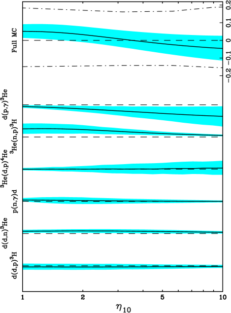
FIG. 16.: Fractional changes (solid curves) and 95% confidence intervals (shaded regions) in ³He/H from our full Monte Carlo calculation and from Monte Carlo studies of individual reactions, relative to the SKM yields and errors (dashed lines). All curves are shown on the same scale.

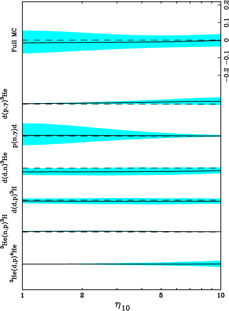
FIG. 17.: Fractional changes (solid curves) and 95% confidence intervals (shaded regions) in (³He+D)/H from our full Monte Carlo calculation and from Monte Carlo studies of individual reactions, relative to the SKM yields (dashed lines). All curves are shown on the same scale.

V conclusions

In summary, we have applied a new Monte Carlo approach to the use of nuclear data in big-bang nucleosynthesis calculations. This approach has the virtues of coupling the results of BBN calculations and their error estimates closely to the available nuclear data, of explicitly handling correlated errors in the data set, of allowing easy use of new data, and of taking some of the data-evaluation process out of human hands. We have also abandoned the explicit conservatism of the previous “industry-standard” error estimation, but the chief virtue of our method is the close coupling of the BBN calculation to the nuclear data, particularly with regard to incorporating new data.

Application of our method has resulted in a reduction in the estimated uncertainty in the BBN calculation. The old estimates of the uncertainties were larger than the quoted uncertainties in recent astronomical observations of BBN nuclides, so that uncertainties in the nuclear inputs dominated inferences from individual observations. Given our prescription, the uncertainties in the calculation are once again smaller than the quoted errors on any of the current observations, and this strengthens the constraints which can be placed on BBN. The constraints that can be derived by applying our calculation to current observations have been discussed in a previous paper [93].

The most important result of our earlier paper is that useful inferences can now be made where nuclear uncertainties formerly precluded any strong conclusions. An example is the question of whether observed lithium abundances are consistent with low deuterium observations, in the absence of lithium depletion on the Spite plateau. The conservative uncertainty estimates would also not allow any determination of the baryon density based on BBN to better than about 10%; our prescription reduces the uncertainty in this quantity so that even given observational errors of a few percent in deuterium, the uncertainty on the baryon density would be dominated by astronomical observations.

We have subsequently found that the calculated BBN yields in Ref. [93] suffer from a programming error which we have now corrected. The error resulted in overestimates of the uncertainties by up to a factor of about 1.5 in Figure 1 of that paper. Discussion in the earlier paper concentrated on uncertainties at $\Omega_{B}h^{2}=0.019$; at that baryon density, correction of the programming error reduces the estimated uncertainty on D/H by a factor of 1.6 and the estimated uncertainty on ⁷Li/H by a factor of 1.2. Consequences of this error for cosmological implications are relatively unimportant, because the uncertainty estimates on our preliminary calculation are already smaller than those on astronomical observations.

With regard to the nuclear data, we point out that any lingering problems with the nuclear database will probably have to be settled by new experiments. The low-energy $p(n,\gamma)d$ cross section is an important gap; the ${}^{3}{\rm He}(d,p)^{4}{\rm He}$ cross section is a less important gap, but it is clearly the case with the worst systematic problems in our nuclear database. Further reactions that contribute to lithium and deuterium yield uncertainties are listed in Sec. IV. The importance of improving various components of the nuclear database relative to improving the astronomical observations can be seen by examining Figs. 14–17.

It is possible to improve on our work. We have explicitly tried to work very directly with the nuclear inputs, and we have therefore avoided theoretical modelling, which is not essential in the face of such copious data. With more theoretical inputs — for example, radiative-capture models and multi-channel $R$-matrix fits — one could include much more data, from higher energies and from scattering channels, and introduce some cross-talk between reaction channels. Solely in terms of gathering and processing data, this would be a much larger undertaking than what we have done. It could probably not be done piecemeal, because important theoretical parameters often have to be determined by examining data in several reaction and scattering channels, and over a wide range in energy. Depending on implementation, theoretical inputs may also present a more difficult problem in terms of propagating errors through to BBN reaction rates.

Improvement may also be possible in our handling of correlated normalization errors. We have also avoided any fancier error estimation than applying quoted errors in a well-defined way. In particulary, we have not fit with floating normalizations because we were wary of altering the most important pieces of information for BBN. In place of floating-normalization methods, we have introduced a Monte Carlo method for making families of smooth curves to characterize data with normalizations that vary in the expected way. Although we do believe that this characterizes the uncertainties in the database in a reasonable way, it is worth noting that the individual curve fitted through each realization of the data does not recognize the presence of correlated errors.

In conclusion, our results indicate that our method of coupling BBN error estimates to the nuclear data may be fruitful not only for providing a useful and unambiguous prescription for such error estimates, but also for making comparison between light-element abundances and BBN calculations more meaningful. While our prescription for handling the nuclear data is not unique, it is simple, repeatable, and direct. Such a method is needed for the program of “precision cosmology.” We hope that our proposal will result at least in a more critical stance toward uncertainty estimates in BBN, and perhaps improved prescriptions that incorporate the better qualities of our method.

- [1] C. J. Copi, D. N. Schramm, and M. S. Turner, Science 267, 192 (1995).
- [2] S. Burles and D. Tytler, Astrophys. J. 499, 699 (1998).
- [3] S. Burles and D. Tytler, Astrophys. J. 507, 732 (1998).
- [4] H. Reeves, J. Audouze, W. A. Fowler, and D. N. Schramm, Astrophys. J. 179, 909 (1973).
- [5] D. N. Schramm and M. S. Turner, Rev. Mod. Phys. 70, 303 (1998).
- [6] R. V. Wagoner, W. A. Fowler, and F. Hoyle, Astrophys. J. 148, 3 (1967).
- [7] R. V. Wagoner, Astrophys. J. 179, 343 (1973).
- [8] L. H. Kawano, FERMILAB-PUB-88/34-A, 1988, (unpublished).
- [9] L. H. Kawano, FERMILAB-PUB-92/04-A, 1992, (unpublished).
- [10] L. M. Krauss and P. Romanelli, Astrophys. J. 358, 47 (1990).
- [11] M. S. Smith, L. H. Kawano, and R. A. Malaney, Astrophys. J. Suppl. 85, 219 (1993), denoted SKM through much of the text.
- [12] K. Jedamzik and G. M. Fuller, Astrophys. J. 452, 33 (1995).
- [13] H. Kurki-Suonio, K. Jedamzik, and G. J. Mathews, Astrophys. J. 479, 31 (1997).
- [14] C. R. Brune, R. W. Kavanagh, and C. Rolfs, Phys. Rev. C 50, 2205 (1994).
- [15] G. J. Schmid, B. J. Rice, R. M. Chasteler, M. A. Godwin, G. C. Kiang, L. L. Kiang, C. M. Laymon, R. M. Prior, D. R. Tilley, and H. R. Weller, Phys. Rev. C 56, 2565 (1997).
- [16] L. Ma, H. J. Karwowski, C. R. Brune, Z. Ayer, T. C. Black, J. C. Blackmon, E. J. Ludwig, M. Viviani, A. Kievsky, and R. Schiavilla, Phys. Rev. C 55, 588 (1997).
- [17] C. Brune, K. I. Hahn, R. W. Kavanagh, and P. R. Wrean, Phys. Rev. C 60, 015801 (1999).
- [18] W. A. Fowler, G. R. Caughlan, and B. A. Zimmerman, Ann. Rev. Astron. Astrophys. 5, 525 (1967).
- [19] W. A. Fowler, G. R. Caughlan, and B. A. Zimmerman, Ann. Rev. Astron. Astrophys. 13, 69 (1975).
- [20] M. J. Harris, W. A. Fowler, G. R. Caughlan, and B. A. Zimmerman, Ann. Rev. Astr. Ap. 21, 165 (1983).
- [21] G. R. Caughlan and W. A. Fowler, At. Data Nucl. Data Tables 40, 283 (1988).
- [22] G. Fiorentini, E. Lisi, S. Sarkar, and F. L. Villante, Phys. Rev. D 58, 063506 (1998).
- [23] W. H. Press, S. A. Teukolsky, W. T. Vetterling, and B. P. Flannery, Numerical Recipes, 2nd ed. (Cambridge University Press, New York, 1992).
- [24] R. Lopez and M. S. Turner, Phys. Rev. D 59, 103502 (1999).
- [25] EXFOR Systems Manual: Nuclear Reaction Data Exchange Format, Nuclear Data Centers Network, National Nuclear Data Center, Brookhaven National Laboratory, Upton, NY, 1996, report No. BNL-NCS-63330, compiled and edited by V. McLane.
- [26] C. de Boor, A Practical Guide to Splines (Springer, New York, 1978).
- [27] G. D’Agostini, Nucl. Instrum. Meth. A 346, 306 (1994).
- [28] ENDF/B-VI Summary Documentation, Cross Section Evaluation Working Group, National Nuclear Data Center, Brookhaven National Laboratory, Upton, NY, 1991, edited by P. F. Rose.
- [29] G. M. Hale, D. C. Dodder, E. R. Siciliano, and W. B. Wilson, Los Alamos National Laboratory, ENDF/B-VI evaluation, Mat # 125, Rev. 2, Oct. 1997; retrieved from the ENDF database at the NNDC Online Data Service.
- [30] T. S. Suzuki, Y. Nagai, T. Shima, T. Kikuchi, H. Sato, T. Kii, and M. Igashira, Astrophys. J. 439, L59 (1995).
- [31] Y. Nagai, T. S. Suzuki, T. Kikuchi, T. Shima, T. Kii, H. Sato, and M. Igashira, Phys. Rev. C 56, 3173 (1997).
- [32] S. F. Mughabghab, M. Divadeenam, and N. E. Holden, Neutron Cross Sections (Academic Press, New York, 1981), Vol. 1.
- [33] G. Hale, private communication.
- [34] G. M. Bailey, G. M. Griffiths, M. A. Olivo, and R. L. Helmer, Can. J. Phys. 48, 3059 (1970).
- [35] G. M. Griffiths, M. Lal, and C. D. Scarfe, Can. J. Phys. 41, 724 (1963).
- [36] M. Viviani, R. Schiavilla, and A. Kievsky, Phys. Rev. C 54, 596 (1996).
- [37] G. M. Griffiths, E. A. Larson, and L. P. Robertson, Can. J. Phys. 40, 402 (1962).
- [38] R. E. Brown and N. Jarmie, Phys. Rev. C 41, 1391 (1990).
- [39] A. Krauss, H. W. Becker, H. P. Trautvetter, and C. Rolfs, Nucl. Phys. A465, 150 (1987).
- [40] A. S. Ganeev, A. M. Govorov, G. M. Osetinskii, A. N. Rakivnenko, I. V. Sizov, and V. S. Siksin, Sov. J. At. Energy. Suppl. 5, 21 (1958).
- [41] G. Preston, P. F. D. Shaw, and S. A. Young, Proc. Roy. Soc. 226, 206 (1954).
- [42] First Research Group, Chin. J. Nuc. High En. Phys., 9, 723, 1985, original in Chinese; all information from CSISRS.
- [43] W. Grüebler, V. König, P. A. Schmelzbach, B. Jenny, and J. Vybiral, Nucl. Phys. A369, 381 (1981).
- [44] K. G. McNeill and G. M. Keyser, Phys. Rev. 81, 602 (1951).
- [45] S. B. Borzakov, H. Malecki, L. B. Pikel’ner, M. Stempinski, and E. I. Sharapov, Sov. J. Nucl. Phys. 35, 307 (1982).
- [46] D. G. Costello, S. J. Friesenhahn, and W. M. Lopez, Nucl. Sci. Eng. 39, 409 (1970).
- [47] J. H. Coon, Phys. Rev. 80, 488 (1950).
- [48] R. Batchelor, R. Aves, and T. H. R. Skyrme, Rev. Sci. Inst. 26, 1037 (1955).
- [49] J. H. Gibbons and R. L. Macklin, Phys. Rev. 114, 571 (1959).
- [50] V. P. Alfimenkov et al., JINR, R3-80-394, 1980.
- [51] D. B. Gayther, Ann. Nucl. Energy 4, 515 (1977).
- [52] G. P. Lamaze, R. A. Schrack, and O. A. Wasson, Nucl. Sci. Eng. 68, 183 (1977).
- [53] R. E. Brown, N. Jarmie, and G. M. Hale, Phys. Rev. C 35, 1999 (1987).
- [54] N. Jarmie, R. E. Brown, and R. A. Hardekopf, Phys. Rev. C 29, 2031 (1984).
- [55] S. J. Bame, Jr. and J. E. Perry, Jr., Phys. Rev. 107, 1616 (1957).
- [56] D. L. Allan and J. J. Poole, Proc. Roy. Soc. A204, 488 (1951).
- [57] E. M. Balabanov, I. I. Barit, L. N. Katsaurov, I. M. Frank, and I. V. Shtranikh, Sov. J. At. Energy. Suppl. 5, 43 (1958).
- [58] A. P. Kobzev, V. I. Salatskiy, and S. A. Telezhnikov, Sov. J. Nucl. Phys. 3, 774 (1966).
- [59] T. W. Bonner, J. P. Conner, and A. B. Lillie, Phys. Rev. 88, 473 (1952).
- [60] L. Zhichang, Y. Jingang, and D. Xunliang, Chin. J. Sci. Tech. At. Energy 3, 229 (1977), original in Chinese; from CSISRS database.
- [61] W. Möller and F. Besenbacher, Nucl. Instrum. Meth. 168, 111 (1980).
- [62] R. R. Arnold, J. A. Phillips, G. A. Sawyer, E. J. Stovall, Jr., and J. L. Tuck, Phys. Rev. 93, 483 (1954).
- [63] U. Schröder, S. Engstler, A. Krauss, K. Neldner, C. Rolfs, and E. Somorjai, Nucl. Instrum. Meth. B40/41, 466 (1989).
- [64] H. Kräwinkel et al., Z. Phys. A304, 307 (1982).
- [65] M. Hilgemeier, H. W. Becker, C. Rolfs, H. P. Trautvetter, and J. W. Hammer, Z. Phys. A329, 243 (1988).
- [66] P. D. Parker and R. W. Kavanagh, Phys. Rev. 131, 2578 (1963).
- [67] K. Nagatani, M. R. Dwarakanath, and D. Ashery, Nucl. Phys. A128, 325 (1969).
- [68] T. K. Alexander, G. C. Ball, W. N. Lennard, H. Geissel, and H. B. Mak, Nucl. Phys. A427, 526 (1984).
- [69] J. L. Osborne, C. A. Barnes, R. W. Kavanagh, R. M. Kremer, G. J. Mathews, J. L. Zyskind, P. D. Parker, and A. J. Howard, Nucl. Phys. A419, 115 (1984).
- [70] R. G. H. Robertson, P. Dyer, T. J. Bowles, C. J. Maggiore, and S. M. Austin, Phys. Rev. C 27, 11 (1983).
- [71] H. Volk, H. Kräwinkel, R. Santo, and L. Wallek, Z. Phys. A310, 91 (1983).
- [72] E. G. Adelberger et al., Rev. Mod. Phys. 70, 1265 (1998).
- [73] H. D. Holmgren and R. L. Johnston, Phys. Rev. 113, 1556 (1959).
- [74] U. Schröder, A. Redder, C. Rolfs, R. E. Azuma, L. Buchmann, C. Campbell, J. D. King, and T. R. Donoghue, Phys. Lett. B 192, 55 (1987).
- [75] G. M. Griffiths, R. A. Morrow, P. J. Riley, and J. B. Warren, Can. J. Phys. 39, 1397 (1961).
- [76] S. Burzyński, K. Czerski, A. Marcinkowski, and P. Zupranski, Nucl. Phys. A473, 179 (1987).
- [77] H. Utsunomiya et al., Phys. Rev. Lett. 65, 847 (1990).
- [78] K. I. Hahn, C. R. Brune, and R. W. Kavanagh, Phys. Rev. C 51, 1624 (1995).
- [79] K. K. Sekharan, H. Laumer, B. D. Kern, and F. Gabbard, Nucl. Instrum. Meth. 133, 253 (1976).
- [80] R. Taschek and A. Hemmendinger, Phys. Rev. 74, 373 (1948).
- [81] H. Spinka, T. Tombrello, and H. Winkler, Nucl. Phys. A164, 1 (1971).
- [82] C. C. Lee, J. Kor. Phys. Soc. 2, 1 (1969), original in Korean; data from CSISRS.
- [83] C. Rolfs and R. W. Kavanagh, Nucl. Phys. A455, 179 (1986).
- [84] S. Engstler, G. Raimann, C. Angulo, U. Greife, C. Rolfs, U. Schröder, E. Somorjai, B. Kirch, and K. Langanke, Z. Phys. A342, 471 (1992).
- [85] J. F. Harmon, Nucl. Instrum. Meth. B40/41, 507 (1989).
- [86] C. Angulo et al., Nucl. Phys. A656, 3 (1999).
- [87] P. Bonifacio and P. Molaro, Mon. Not. R. Astron. Soc. 285, 847 (1997).
- [88] Y. I. Izotov and T. X. Thuan, Astrophys. J. 500, 188 (1998), also see ibid 497, 227 (1998).
- [89] K. A. Olive, E. Skillman, and G. Steigman, Astrophys. J. 483, 788 (1998), also see K. A. Olive and G. Steigman, Astrophys. J. (Suppl. ) 97, 490 (1995).
- [90] D. N. Schramm, in Generation of Large-Scale Cosmological Structure, edited by D. N. Schramm and P. Galeotti (Kluwer, Dordrecht, 1997), p. 127.
- [91] R. T. Rood, T. M. Bania, D. S. Balser, and T. L. Wilson, Space Science Reviews 84, 185 (1998).
- [92] D. S. Balser, T. M. Bania, R. T. Rood, and T. L. Wilson, Astrophys. J. 510, 759 (1998).
- [93] S. Burles, K. M. Nollett, J. W. Truran, and M. S. Turner, Phys. Rev. Lett. 82, 4176 (1999).