Stellar Dynamics in the Galactic centre:
Proper Motions and Anisotropy

Abstract

We report a new analysis of the stellar dynamics in the Galactic centre, based on improved sky and line-of-sight velocities for more than one hundred stars in the central few arcseconds from the black hole candidate SgrA*. The main results are:

$\bullet$ Overall the stellar motions do not deviate strongly from isotropy. For those 32 stars with a determination of all three velocity components the absolute, line of sight and sky velocities are in good agreement, consistent with a spherical star cluster. Likewise the sky-projected radial and tangential velocities of all 104 proper motion stars in our sample are also consistent with overall isotropy.

$\bullet$ However, the sky-projected velocity components of the young, early type stars in our sample indicate significant deviations from isotropy, with a strong radial dependence. Most of the bright HeI emission line stars at separations from 1” to 10” from SgrA* are on tangential orbits. This tangential anisotropy of the HeI stars and most of the brighter members of the IRS16 complex is largely caused by a clockwise (on the sky) and counter-rotating (line of sight, compared to the Galaxy), coherent rotation pattern. The overall rotation of the young star cluster probably is a remnant of the original angular momentum pattern in the interstellar cloud from which these stars were formed.

$\bullet$ The fainter, fast moving stars within $\approx{}1^{\prime\prime}$ from SgrA* appear to be largely moving on radial or very elliptical orbits. We have so far not detected deviations from linear motion (i.e. acceleration) for any of them. Most of the SgrA* cluster members also are on clockwise orbits. Spectroscopy indicates that they are early type stars. We propose that the SgrA* cluster stars are those members of the early type cluster that happen to have small angular momentum and thus can plunge to the immediate vicinity of SgrA*.

$\bullet$ We derive an anisotropy-independent estimate of the Sun-Galactic centre distance between 7.8 and 8.2 kpc, with a formal statistical uncertainty of $\pm 0.9{\ {\rm kpc}}$.

$\bullet$ We explicitly include velocity anisotropy in estimating the central mass distribution. We show how Leonard-Merritt and Bahcall-Tremaine mass estimates give systematic offsets in the inferred mass of the central object when applied to finite concentric rings for power law clusters. Corrected Leonard-Merritt projected mass estimators and Jeans equation modelling confirm previous conclusions (from isotropic models) that a compact central mass concentration (central density $\geq$10 ^12.6M_☉ pc${}^{{\ -3}}$) is present and dominates the potential between 0.01 and 1 pc. Depending on the modelling method used the derived central mass ranges between 2.6 and $3.3\times 10^{{\ 6}}M_{{\sun}}$ for R${}_{{\sun}}=8.0{\ {\rm kpc}}$.

1 Introduction

High spatial resolution observations of the motions of gas and stars have in the past decade substantially strengthened the evidence that central dark mass concentrations reside in many and perhaps most nuclei of nearby galaxies (Kormendy and Richstone 1995, Magorrian et al. 1998, Richstone et al. 1998). These dark central masses are very likely massive black holes. The most compelling evidence for this assertion comes from the dynamics of water vapor maser cloudlets in the nucleus of NGC 4258, and from the stellar dynamics in the centre of our own Galaxy (Greenhill et al. 1995, Myoshi et al. 1995, Eckart and Genzel 1996, 1997, Genzel et al. 1997, Ghez et al. 1998). In both cases the gas and stellar dynamics indicate the presence of an unresolved central mass whose density is so large that it cannot be stable for any reasonable length of time unless it is in form of a massive black hole (Maoz 1998).
The case of the Galactic centre is particularly intriguing, as it is very close (8 kpc). With the highest spatial resolution observations presently available in the near-infrared ($\leq$0.1”), spatial scales of a few light days can be probed. Measurements of both line-of-sight velocities (through Doppler shifts in spectral lines) and sky/proper motions are available and pose very strong constraints on the central mass concentration. The following results have emerged.

$\bullet$ The mean stellar velocities (or velocity dispersions) follow a Kepler law ($\langle$v${}^{{\ 2}}\rangle$ $\propto$ R${}^{{\ -1}}$) from projected radii R from 0.1” to $\approx$20”, providing compelling qualitative evidence for the presence of a central point mass (Sellgren et al. 1990, Krabbe et al. 1995, Haller et al. 1996, Genzel et al. 1996, 1997, Eckart and Genzel 1996, 1997, Ghez et al. 1998).

$\bullet$ The positions of the dynamical centre (maximum velocity dispersion) and of the maximum stellar surface number density agree with the position of the compact radio source SgrA* (size less than a few AU, Lo et al. 1998, Bower and Backer 1998) to within $\pm$0.1” (Ghez et al. 1998).

$\bullet$ Projected mass estimators and Jeans equation modeling of the stellar velocity data indicate that the central mass ranges between 2.2 and $3\times 10^{{\ 6}}M_{\odot}$. It has a mass to luminosity ratio of $M/L>100M_{\sun}/L_{\sun}$ and a density $\geq 2\times 10^{{\ 12}}M_{\sun}{\ {\rm pc}}^{{\ -3}}$ (Genzel et al. 1997, Ghez et al. 1998).

The Galactic centre mass modeling has so far assumed that the stellar velocity ellipsoid is isotropic. An initial comparison of line-of-sight and proper motion velocity dispersions indeed suggests that there are no coarse deviations from isotropy (Eckart and Genzel 1996, 1997). However, to make a more detailed assessment, it is necessary to obtain more accurate stellar motions than were available two years ago. These improved motions -for line-of-sight and sky components - are now in hand and will be analysed in the present paper.

2 Observations and Data Analysis

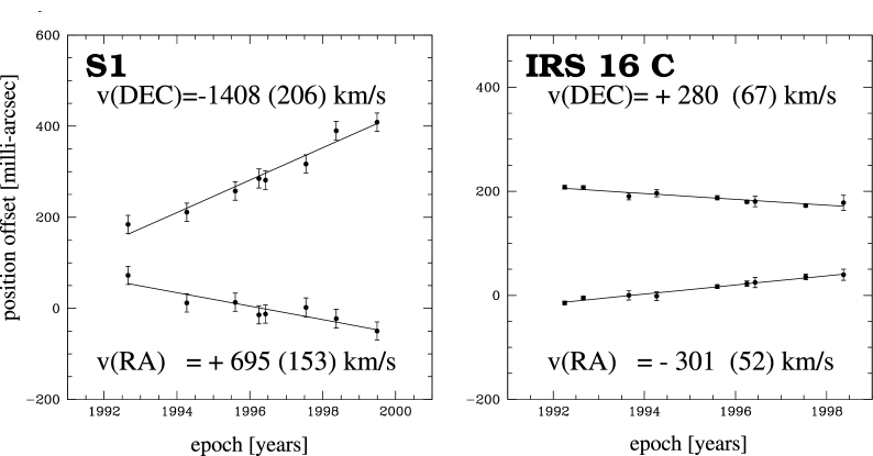
Figure 1: Examples of the proper motions derived from the 1992 to 1998 data NTT data sets obtained with the MPE SHARP camera. Shown are position-time plots for source S1 close to SgrA* (left) and the bright HeI emission line star IRS16 C (right). The two panels show x-(=RA) and y-(=Dec) position offsets, along with the best-fitting proper motions (straight lines). For each epoch the average and 1$\sigma$ dispersion of a number position measurements are plotted.

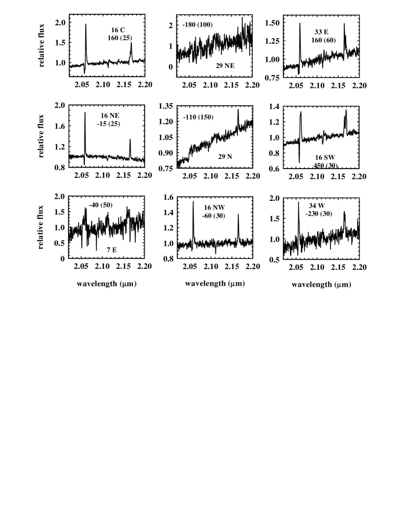
Figure 2: K-band spectra of early type stars in the central $\approx{}10^{\prime\prime}$ obtained in spring 1996 with the MPE 3D spectrometer on the ESO-MPG 2.2m telescope . The spectral resolving power is $\lambda$/$\Delta\lambda=2000$, Nyquist sampled at twice that resolution. Most of the spectra were obtained by subtracting from the ‘on-star‘ spectrum ($0.3^{{\prime\prime}}$ to $1.2^{\prime\prime}$ aperture) an ‘off-star‘ spectrum scaled to the same area, in order to remove local nebular emission. The name is given for each star, as is the stellar velocity in km/s, with the 1 $\sigma$ uncertainty in parentheses.

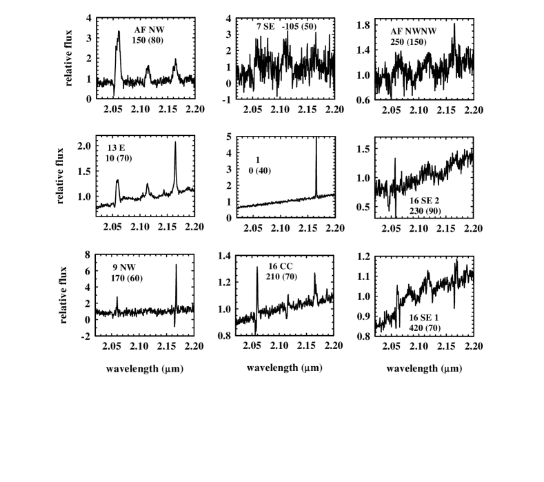
Figure 3: see Fig. (2)

2.1 Proper Motions

In our earlier papers (Eckart et al. 1992, 1993, 1994, 1995) we have described the data acquisition and reduction that allowed us to obtain stellar positions with a precision of $\approx$10 milli-arcseconds per measurement (Eckart and Genzel 1996, 1997, Genzel et al. 1997). We used the MPE-SHARP camera (Hofmann et al. 1993) on the 3.5m New Technology Telescope (NTT) of the European Southern Observatory (ESO). SHARP contains a 256² pixel NICMOS 3 detector. Each pixel projects to 25 or 50 milli-arcseconds on the sky in order to (over-)sample the $\approx$ 0.15” FWHM diffraction limited image of the NTT in K-band. The raw data for each data set consist of several thousands of short exposure frames (0.3 to 0.5 seconds integration time). First we processed the data from nights with very good seeing (0.4 to 0.8” ) in the standard manner (dead pixel correction, sky subtraction, flat-fielding etc.). Next we co-added with the simple-shift-and-add algorithm (SSA: for details see Christou 1991 and Eckart et al. 1994). The individual short exposure frames typically contain only a few bright speckles so that the SSA algorithm is well suited for our purpose. The bright infrared sources IRS7 or IRS16NE serve as reference sources. For the present study we analysed $\approx$82 independent data sets from a total of 9 observing runs in 1992.25, 1992.65, 1993.65, 1994.27, 1995.6, 1996.25, 1996.43, 1997.54 and 1998.37. For the central arcsecond region around SgrA* (the ’SgrA* cluster’) we also analysed an additional data set from 1999.42. Eckart and Genzel (1996, 1997) and Genzel et al. (1997 have previously analysed and discussed the data until 1996.43.

The diffraction limited core of the stellar SSA images contains up to 20 percent of the light. Determinations of the relative pixel offsets from IRS16NE in raw SSA images or from diffraction limited maps after removing the seeing halo give consistent results (see Eckart and Genzel 1996, 1997 for details). These ‘CLEANed’ SSA maps produce similar results as other data reductions (Knox-Thompson, triple correlation) but give much higher dynamical range (see Eckart et al. 1994 for a detailed discusssion). This is essential in the crowded Galactic centre region where the difference between the brightest and faintest stars in our images is almost 10 magnitudes. We solved for the relative offsets, rotation angle, and for the linear and quadratic distortions between individual frames from an over-determined system of non-linear equations for a reference list of relatively isolated bright stars (Eckart and Genzel 1996, 1997). Our final near-infrared reference frame is tied to an accuracy of $\pm$30 milli-arcsecs to the VLA radio frame through 5 stars that show SiO and H ₂O maser activity and are common to both wavelength bands (Menten et al. 1997). The resulting combined systematic errors in our proper motion velocity estimates probably are about 30 km/s. In the best cases these systematic effects now dominate the error budget.

The new 1997 and 1998 data sets are in excellent agreement with the extrapolation of the data we have published before and significantly improve the uncertainties. As examples we show in Fig. (1) the relative RA- and Dec-position offsets as a function of time between 1992 and 1998 for two selected stars. IRS16 C is a bright and isolated, HeI emission line star (Krabbe et al. 1991, 1995). Its position vs. time diagram in Fig. (1) is an example of the quality of the data on bright isolated stars. S1 is a faint star in the ‘SgrA* cluster’ that is very close to SgrA* ($\approx$0.1”). It shows the fastest proper motion ($\approx$1470 km/s) in the entire sample.

2.2 3D Spectroscopy

We observed the Galactic centre with the MPE-3D near-infrared spectrometer (Weitzel et al. 1996) in conjunction with the tip-tilt adaptive optics module ROGUE (Thatte et al. 1995). 3D is a field imaging spectrometer which obtains spectra simultaneously for 256 spatial pixels covering a square region of the sky (16x16 pixels). The fill factor is over 95Ḟor further details of the instrument and data reduction we refer to Weitzel et al. (1996). We observed the Galactic centre in March 1996 at the 2.2m ESO-MPG telescope on La Silla, Chile. During the run the seeing on the seeing monitor ranged between 0.3” and 0.8”. The pixel scale was 0.3”. We observed the short-wavelength part of the K-band (1.9-2.2$\mu$m) at $\lambda$/$\Delta\lambda$=2000, Nyquist sampled with two settings of a piezo driven flat mirror. We covered the central $\approx$16”x10” centered on SgrA* by an overlapping set of frames, each with a field of view of 4.8”x4.8”. At each position we set up a sequence on-source (piezo step 1), off-source (piezo step 1), on-source (piezo step 2), off-source (piezo step 2) etc. with an integration time per step of 200 seconds. Due to the combined effects of seeing and pixel scale the resulting FWHM spatial resolution of the final combined data set was 0.6”. We employed the standard 3D data analysis package (based on GIPSY: van der Hulst et al. 1992). We performed wavelength calibration, sky subtraction, spectral and spatial flat fielding, dead and hot pixel correction and division by a reference stellar spectrum obtained during the observations. We corrected for the effects of a spatially varying fringing or ‘channel’ spectrum due to interference in the saphire coating of the NICMOS 3 detector by applying suitable flat fields from a set of flatfields at different settings of the piezo mirror. Based on obervations of calibration lamps and OH sky lines during the different observing nights the final velocity calibration is accurate to $\pm 16km/s.$

In the observed field we identified 21 emission line stars from continuum subtracted images of the 2.058$\mu$m n=2 ¹P- n=2 ¹S and 2.11$\mu$m n=4 ^3,1S - n=3 ^3,1P HeI lines and the 2.166$\mu$m n=7-4 HI (Br$\gamma$) line. Most of the stars are identical with those found in the $\approx$1”, R=1000 3D data set of Krabbe et al. (1995) and Genzel et al. (1996) ( see also Blum, Sellgren and dePoy 1995 a,b and Haller et al.1986) but the resolution, quality and nebular rejection is now much superior. Three new stars were identified: (-2.1”, -4.1”) (13S SE), (+1.6”, +0.3”) (16 CC) and (-8.3”, -5.7”) (all offsets are in RA and Dec from SgrA*). We extracted from the data cube spectra of individual stars by typically averaging 3 to 16 pixels on the star, for effective apertures between 0.3” and 1.2”. In most cases, we subtracted a suitable ‘off-star’ spectrum (scaled to the same aperture area) to eliminate the effect of local nebular line emission. Fig. (2) and Fig. (3) show the final spectra for 18 of the 21 stars.

To determine stellar velocities we fitted Gaussians to the 2.058$\mu$m and 2.11$\mu$m HeI lines and the 2.166$\mu$m Br$\gamma$ line.In a few cases we also used in addition the 2.137/2.143$\mu$m MgII lines and the 2.189$\mu$m HeII line. A number of the stars clearly display P-Cyg profiles in the 2.058$\mu$m HeI transition (Fig. (2) and Fig. (3)) . In these cases we fitted the profile with a double Gaussian (absorption and emission). As the absorption structure is well resolved an unambiguous emission line centroid (assumed to be the stellar velocity) can thus be easily obtained. For most stars we determined the final stellar velocities from averaging the values obtained from 3 (or 4) lines. The agreement between the fits to the different lines is generally good or even excellent. We list the final velocities in Table 1 and the insets of Fig. (2) and Fig. (3). The new velocity determinations agree with those of Genzel et al. (1996) but the uncertainties are typically half of those in our earlier work. The best cases have an uncertainty of $\pm$25 km/s.

2.3 A Homogenized Data Set

To obtain a homogenized ‘best’ data set of stellar velocities for further analysis we combined the new 1992-1998 NTT proper motions and 2.2m line-of-sight velocity data described in the last two paragraphs with the 1995-1997 Keck proper motion data of Ghez et al. (1998) and with other relevant line-of-sight velocity data sets (see Genzel et al. 1996 and references therein). Table 1 gives the results. The following explanations and comments for Table 1 are in order.

$\bullet$ Columns 1 through 3 contain the projected separation R, x(=RA)-offset and y (=Dec)-offset between star and SgrA* (epoch 1994/1995, all in arcseconds). As for the NTT, the Keck astrometry is established with H₂O/SiO maser stars that are visible in both wavelength bands and is accurate to $\pm$10 milli-arcseconds (see Ghez et al. 1998, Menten et al. 1997).

$\bullet$ Columns 4 through 15 contain the x- and y-proper motions and their respective 1$\sigma$ errors (km/s, for a Sun-Galactic centre distance of $R_{{\sun}}=8.0{{\rm kpc}}$). Whenever two measurements are available, we first list the velocity from the Keck observations and then that from the NTT observations. Columns 12 through 15 give the final combined proper motions obtained from averaging motions from the two sets (if available) with 1/$\sigma^{{2}}$ weighting. The agreement between Keck and NTT data sets generally is very good (see discussion by Ghez et al. 1998) and is in accordance with the measurement uncertainties. We thus assume that the final measurement error of the combined set is given by 1/ $\surd$ (1/$\sigma_{{1}}^{{2}}$ + 1/$\sigma_{{2}}^{{2}}$). We have found, however, from a comparison of the two data sets that stars with $>$200 km/s velocity uncertainty at $R\geq 1^{\prime\prime}$ (and $>$400 km/s at $R\leq 1^{\prime\prime}$) are highly unreliable. We therefore have eliminated such stars from the final set.

$\bullet$ Columns 16 and 17 give the line of sight velocity and its 1$\sigma$ error.

$\bullet$ Column 18 assigns a weight to each data point, based on its reliability, the velocity errors and the agreement between different data sets. The weight is approximately proportional to 1/error² as appropriate for white noise but ‘quantized’ in order to not place too much weight on the few data points with the smallest statistical errors. While this weighting scheme is subjective it is in our opinion a fair representation of the quality of the different data points in the presence of significant systematic errors. We have also tried another, more formal weighting scheme. Here we have assigned the weight $w=1/(1+({{\rm error}}/\sigma_{{0}})^{{2}}$), where ‘error’ is the x/y-averaged proper motion velocity uncertainty. $\sigma_{{0}}=250R^{{-0.5}}$ is a measure of the sample dispersion at R. This weighting scheme also gives essentially the same weights for different data points as long as their individual errors are much smaller than the sample velocity dispersion. For large errors the weight scales as 1/error² as for white noise. We have applied both weighting schemes in the various estimates discussed in the text. The results are basically identical.

$\bullet$ Column 19 lists the ‘popular’ name of the star.

$\bullet$ Column 20 lists an identification; ‘p’ stands for a star with a measured proper motion, ‘early’ denotes that the star is a young early type star (e.g. HeI/HI emission lines), and ‘CO’ denotes that the star is a late type star.

$\bullet$ Column 21 lists the source(s) of measurement for the specific data point (Keck (K) and NTT (N) for proper motions, LaSilla (LS), or ‘all’).

$\bullet$ Column 22 lists the K-magnitude of the star, and column 23 makes a statement on its variability. If available, we used the K-magnitudes from the comprehensive variability study of Ott et al. (1999), otherwise we list the magnitudes of Ghez et al. (1998), corrected for $\delta$m_K=-0.4 to account for a small calibration offset between the Ott et al. and Ghez et al. sets. If the value in the last column is 0, the star was not or not significantly variable in the 1992 to 1998 monitoring campaign of Ott et al. A value of 1 indicates that the star showed a statistically significant but weak variability. A value of 2 indicates that the star was strongly variable in the Ott et al. observations.

3 Kinematics of the Galactic Centre Star Cluster

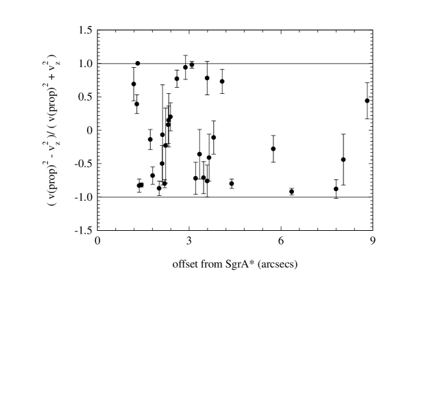
Figure 4: The anisotropy parameter $\gamma_{{pz}}=(v_{{prop}}^{{2}}-v_{{z}}^{{2}})/(v_{{prop}}^{{2}}+v_{{z}}^{{2}})$ for all 32 stars with all three velocity components measured. Error bars are determined through error propagation from the velocity uncertainties in Table 1.

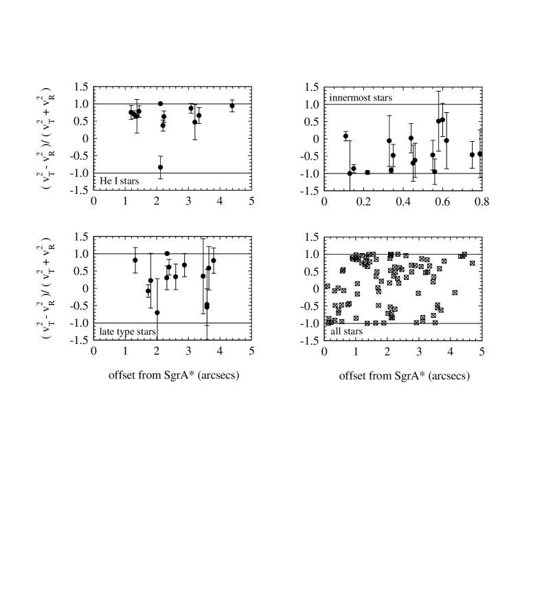
Figure 5: The anisotropy parameter $\gamma_{{TR}}=(v_{{T}}^{{\ 2}}-v_{{R}}^{{2}})/(v_{{T}}^{{2}}+v_{{R}}^{{2}}$) for the 12 HeI stars within $R\leq 5``$ (top left), for the 14 late type stars within $R\leq 5``$ (bottom left), for all stars inside 5“ with proper motions (bottom right) and for stars within $R\leq 0.8``$ of SgrA* (top right). Error bars are determined through error propagation from the velocity uncertainties in Table 1.

The velocity determinations in Table 1 are significantly improved over our earlier work and over Ghez et al. (1998). Many light-of-sight and sky velocities now have errors less than 50 ${\rm km\,s}^{-1}$, with the best velocity determinations ($\pm$20 to 25 km/s) mainly limited by systematic effects (e.g. establishing reference frame from the moving stars themselves and removing distortions in the imaging), rather than by statistical errors (positional accuracy of stellar positions). Of the $2\times 104$ proper motions in Table 1, 48 (23%) are determined to 4$\sigma$ or better. 5 proper motions are determined at the $\geq$10$\sigma$ level. Of the 227 line-of-sight velocities 38 (17%) are determined to 4$\sigma$ or better. For 14 (of 29) HeI emission line stars and for 18 late type stars we now have determinations of all three velocity components. With this improved data set it is now possible to investigate in more detail the kinematic parameters of individual stars and/or small groups of stars. In order to remove as well as possible measurement and calibration bias and zero point offsets, we subtract in all of our calculations below for each velocity measurement i the mean velocity of the sample $\langle v\rangle$ linearly and the velocity uncertainty error (v_i) in squares when computing velocity dispersions etc.,

$$(v_{{i}}^{{2}})_{{\rm intrinsic}}=(\{v_{{i}}-\langle v\rangle\}^{{2}})_{{\rm measured}}-error^{{2}}(v_{{i}}).$$ (1)

3.1 Tests for Anisotropy

As proposed by Eckart and Genzel (1996, 1997), a first simple (but coarse) test for anisotropy in the data (and/or a Sun-Galactic centre distance significantly different from $R_{{\sun}}=8{{\rm kpc}}$) is to compare the sky and line-of-sight velocities of individual stars. Fig. (4) is a plot of $\gamma_{{pz}}$=(v${}_{{prop}}^{{2}}$ - v${}_{{z}}^{{2}}$)/ (v${}_{{prop}}^{{2}}$ + v${}_{{z}}^{{2}}$) as a function of projected separation R for the 32 stars with three measured velocities. Here v_prop is the root mean square of the x- and y-sky motions, $v_{{z}}$ is the line-of-sight motion. In this plot stars with $\gamma_{{pz}}=-1$ have v${}_{{z}}\gg v_{{prop}}$ stars with $\gamma_{{pz}}$=+1 have $v_{{z}}\ll v_{{prop}}$. Fig. (4) shows no obvious sign for such an anisotropy. This is probably not surprising as the line-of-sight and sky velocities both contain linear combinations of the intrinsic radial and tangential components of the velocity ellipsoid. The result in Fig. (4) that the sample expectation value for the proper motion velocity dispersion is the same (within statistical uncertainties) as the line-of-sight dispersion, $<v_{prop}^{2}>\simeq<v_{z}^{2}>$, is consistent with the assumption that we are observing a spherically symmetric cluster. The virial theorem guarantees that this results holds independent of internal anisotropy (see equations  (7)  (8)  (9)) .

To investigate intrinsic kinematic anisotropies it is therefore necessary to explicitly decompose the observed motions into projections of the intrinsic velocity components. Assuming that the velocity ellipsoid of a selected (sub-) sample of stars separates in spherical coordinates and denoting the components of velocity dispersion parallel and perpendicular/tangential to the radius vector r as $\sigma_{{r}}$ and $\sigma_{{t}}$, the line-of-sight component $\hat{\sigma}_{{z}}(R,z)$ is then given by

$$\hat{\sigma}_{{z}}^{{2}}=\sigma_{{r}}^{{2}}(r)\cos^{{2}}\theta+\sigma_{{t}}^{{2}}(r)\sin^{{2}}\theta,$$ (2)

where $\cos\theta={{{\bf{r}}}}\cdot{{{\bf{z}}\/}}/r$ and ${}{\bf z\/}$ is the unit vector along the line-of-sight. The components of the velocity dispersion parallel (R) and perpendicular (T) to the projected radius vector on the sky R are given by

$$\hat{\sigma}_{{R}}^{{2}}=\sigma_{{r}}^{{2}}(r)\sin^{{2}}\theta+\sigma_{{t}}^{{2}}(r)\cos^{{2}}\theta,$$ (3)

and

$$\hat{\sigma}_{{T}}^{{2}}=\sigma_{{t}}^{{2}}(r)\quad.$$ (4)

Given the spatial density distribution $n(r)$ of the selected sample of stars (assumed to be spherically symmetric) the line-of-sight averaged, density weighted value of the projected radial velocity dispersion of the sample at $R$, $\sigma_{{R}}$, can then be computed from the relationship

$$\Sigma(R)\sigma_{{R}}^{{2}}(R)=\int_{-\infty}^{\infty}n(z)(\sigma_{{r}}^{{2}}(r)\sin^{{2}}\theta+\sigma_{{t}}^{{2}}(r)\cos^{{2}}\theta){{\rm d}{z}}=2\int_{R}^{\infty}[\sigma_{{r}}^{{2}}(r)(R/r)^{{2}}+\sigma_{{t}}^{{2}}(r)(1-(R/r)^{{2}}]\frac{n(r)r{{\rm d}{r}}}{(r^{{2}}-R^{{2}})^{{1/2}}}\quad$$ (5)

where $\Sigma(R)$ is the stellar surface density at R,

$$\Sigma(R)=2\int_{R}^{\infty}\frac{n(r)r{{\rm d}{r}}}{(r^{{2}}-R^{{2}})^{{1/2}}}\quad$$ (6)

Similar equations hold for $\sigma_{{T}}^{{2}}(R)$ and $\sigma_{{z}}^{{2}}(R)$. The global expectation value of the projected radial dispersion is given by

$$\langle\sigma_{{R}}^{{2}}\rangle=(2\pi/N)\int_{0}^{\infty}\int_{0}^{\pi}n(r)r^{{2}}(\sigma_{{r}}^{{2}}(r)\sin^{{2}}\theta+\sigma_{{t}}^{{2}}(r)\cos^{{2}}\theta)\sin\theta{{\rm d}{\theta}}{{\rm d}{r}}=2/3\langle\sigma_{{r}}^{{2}}\rangle+1/3\langle\sigma_{{t}}^{{2}}\rangle\quad,$$ (7)

where N is the number of stars in the selected sample. Likewise one finds

$$\langle\sigma_{{z}}^{{2}}\rangle=(2\pi/N)\int_{0}^{\infty}\int_{0}^{\pi}n(r)r^{{2}}(\sigma_{{r}}^{{2}}(r)\cos^{{2}}\theta+\sigma_{{t}}^{{2}}(r)\sin^{{2}}\theta)\sin\theta{{\rm d}{\theta}}{{\rm d}{r}}=1/3\langle\sigma_{{r}}^{{2}}\rangle+2/3\langle\sigma_{{t}}^{{2}}\rangle,$$ (8)

and

$$\langle\sigma_{{T}}^{{2}}\rangle=\langle\sigma_{{t}}^{{2}}\rangle$$ (9)

(Leonard & Merritt 1989). Deviations of the velocity ellipsoid from isotropy are commonly expressed in terms of the anisotropy parameter $\beta=1-\sigma_{{t}}^{{2}}/\sigma_{{r}}^{{2}}$. Its globally averaged value is given by

$$\langle\beta\rangle=1-\langle\sigma_{{t}}^{{2}}\rangle/\langle\sigma_{{r}}^{{2}}\rangle=3(\langle\sigma_{{R}}^{{2}}\rangle-\langle\sigma_{{T}}^{{2}}\rangle)/(3\langle\sigma_{{R}}^{{2}}\rangle-\langle\sigma_{{T}}^{{2}}\rangle)\quad.$$ (10)

An isotropic cluster ($\langle\beta\rangle$=0) has $\langle\sigma_{{r}}\rangle$=$\langle\sigma_{{t}}\rangle$ and $\langle\sigma_{{R}}\rangle$=$\langle\sigma_{{T}}\rangle$. A cluster with only radial orbits ($\langle\beta\rangle$=1) has $\langle\sigma_{{t}}\rangle$=$\langle\sigma_{{T}}\rangle$=0 or $\langle\sigma_{{R}}\rangle\gg\langle\sigma_{{T}}\rangle$. A cluster with only tangential orbits ($\langle\beta\rangle$ = -$\infty$) has $\langle\sigma_{{r}}\rangle$ =0 and $\langle\sigma_{{R}}\rangle$= $\langle\sigma_{{T}}\rangle$/$\surd$3. Thus radial anisotropy is easier to see in the proper motions than tangential anisotropy. Table 2 gives the values of $\langle\sigma_{{R}}\rangle$, $\langle\sigma_{{T}}\rangle$, $\langle\sigma_{{R}}\rangle$/$\langle\sigma_{{T}}\rangle$ and $\langle\beta\rangle$, computed for all stars with proper motions and for different ranges of projected radii from SgrA*. Errors in these quantities are derived from statistics and error propagation. Below we use Monte Carlo simulations to investigate the uncertainties in the derived anisotropy parameters more throroughly. The proper motions of the entire sample of stars as well as the stars in the range R$\geq$3” are consistent with isotropy. At R=1 to 3” there is a (marginal) trend for the stars to be more on tangential orbits. In the central arcsecond the stars on average appear to be on radial orbits. The statistical significance of this departure from isotropy for the 17 stars at R$\leq$0.8” from SgrA* appears to be 3.3$\sigma$ in terms of propagated errors for $\beta$ (Table 2); however, the Monte Carlo simulations of Section 4.3 below show that the distribution of $\beta$ is very broad and the isotropic $\beta=0$ is still within somewhat more than 1$\sigma$ equivalent for such a small sample. Excluding the faint stars in the SgrA* cluster at R$\leq$ 1” the remaining proper motions between R=1” and 5” deviate from isotropy in the direction of tangential orbits at the 2$\sigma$ level.

A second and more sensitive test for anisotropy is a comparison of the projected radial (v_R) and projected tangential (v_T) components of the sky velocities of individual stars. Fig. (5) gives plots of $\gamma_{TR}=(v_{{T}}^{{2}}-v_{{R}}^{{2}})/(v_{{T}}^{{2}}+v_{{R}}^{{2}})$ for different selections of our data. Considering all 104 proper motions, Fig. (5) (bottom right) indicates a fairly even distribution of $\gamma_{{TR}}$s, without obvious overall bias indicating anisotropy, perhaps a slight predominance of tangential orbits (compare Fig. (9)). The same is true if only the late type stars of the proper motion sample are considered (Fig. ( 5), bottom left).

A different and fairly clearcut picture emerges when one considers the (much younger) early type stars. Fig. (5) (top left) clearly indicates that with one exception all bright HeI emission line stars within R=5” are on projected tangential orbits ($\gamma_{{TR}}$$\approx$+1) and therefore (see the discussion after equation  (10) ), largely on true tangential or circular orbits. In contrast, more than half of the faint (m_K$\approx$13 to 16) stars within 1” of SgrA* (SgrA* cluster) are predominantly on radial ($\gamma_{{TR}}\leq$ 0) orbits (top right panel of Fig. (5)). We conclude that the early type stars in our proper motion set do show significant anisotropy.. We will show below that the main cause of the tangential anisotropy is a global rotation of the early type stars.

3.2 Orbits for the innermost stars

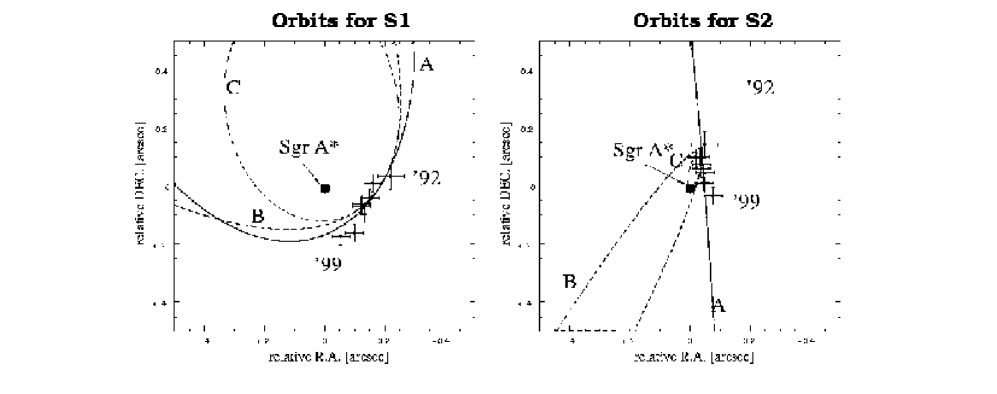
Figure 6: Possible orbits for S1 and S2, the stars closest to SgrA*. The positions of S1(left) and S2 (right) between 1992 and 1999 and their uncertainties are shown as crosses. Three possible bound orbits in the potential of a 2 to $3\times 10^{{6}}M_{{\sun}}$ point mass are shown. Orbit A (continuous curve) has the largest possible separation from SgrA* and orbit B (short dashes) the largest line of sight velocity. The assumption that S1 and S2 are in the same plane of the sky as the central mass and have no line of sight velocity results in the orbit with the largest curvature (orbit C, dash-dotted).

We have also modeled the orbits of several of the individual fast moving stars in the SgrA* cluster. As an example we plot in Fig. (6) the measured 1992-1999 NTT positions of S1 and S2 with respect to SgrA*, along with the projection of a few possible trajectories. The three plotted orbits represent extreme choices of the orbital parameters in the potential of a central compact mass. For orbit A we assumed the largest possible current separation from SgrA* for bound orbits with $v_{z}=0$. For orbit B we took the largest line of sight velocity at $z=0$ under the boundary condition that S1 and S2 are still bound to SgrA*. The assumption that S1/S2 are in the same plane of the sky as the central mass and have no line of sight velocity results in the orbit with the largest curvature (orbit C). Although no unique orbit can yet be determined from the data, our analysis shows that most of the high velocity stars in the SgrA* cluster can be bound to a central mass of $~{}3\times 10^{{6}}M_{{\sun}}$ with a distribution of line of sight positions and velocities that is consistent with the projected dimensions and velocity dispersion of the cluster. Orbits with radii of curvature comparable to their projected radii from SgrA* (orbit C) can already be excluded for these stars. S1, S2 and several other fast moving stars around SgrA* must be on plunging (radial) orbits or on very elliptical/parabolic orbits with semi-axes much greater than the current projected separations from SgrA*, as already indicated by the analysis of the velocities in the preceding paragraph. The stellar orbits in the central cluster will not be simple closed ellipses. Especially for orbits with large eccentricities, node-rotation due to the non-Keplerian potential in the extended stellar cluster as well as relativistic periastron rotations will make the trajectories for the individual stars ‘rosette’-like. A more detailed analysis of orbits has to await longer time baselines for the proper motion measurements and the detection of orbit curvature (= acceleration), as well as measurements of the line of sight velocities of the central stars.

3.3 Anisotropy and Relaxation Time

These deviations from isotropy for the early-type stars are consistent with their young ages as compared to the relaxation time. Within the central stellar core, the two-body relaxation time for a star of mass m₁₀ (in units of 10 M_⊙) is given by

$$t_{{r}}(m)=10^{{7.58}}\sigma_{{100}}^{{3}}/(\rho_{{6.6}}m_{{10}}\{lnN_{{\ast}}/13\})\quad({\rm yrs}).$$ (11)

Here $\rho_{{6.6}}$ is the density of the nuclear star cluster (in units of $4\times 10^{{6}}M_{\sun}{{\rm pc}}^{{-3}}$) and $\sigma_{{100}}$ is the velocity dispersion in units of 100 km/s within the core radius of 0.38 (+0.25,-0.15) pc (Genzel et al. 1996). N_∗ is the number of stars in the core ($\approx{}3to5\times 10^{{5}}$). The life-time of the upper main sequence phase scales approximately as $t_{{ms}}\approx{}10^{{7.2}}m_{{10}}^{{-1.9}}{{\rm yr}}$ and the duration of the red-/blue-giant or supergiant phases is typically 10 to 30% of $t_{{ms}}$ (e.g. Meynet et al. 1994). The ratio of relaxation time to stellar life time thus is

$$\chi=t_{{r}}/t_{{ms}}\approx{}2.4m_{{10}}^{{0.9}}.$$ (12)

A number of authors have shown have shown that the HeI emission line stars are high mass (30 to 120 M_☉), post main sequence blue supergiants (Allen et al. 1990, Krabbe et al. 1991, 1995, Najarro et al. 1994, 1997, Libonate et al. 1995, Blum, Sellgren and dePoy 1995 a,b, Tamblyn et al. 1996, Ott et al. 1999). Their ages range between $t\approx{}2{{\rm and}}9\times 10^{{6}}$ yrs (Najarro et al. 1994, 1997, Krabbe et al. 1995). The massive stars are probably the ‘tip of the iceberg’ of a component of young stars of total mass $\approx$10⁴ M_☉ that were formed a few million years ago in an extended starburst episode (Krabbe et al. 1995). The massive stars are somewhat older than their main sequence age. Their main sequence life time is much greater than the dynamical time scale ($t_{ms}\gg t_{{\rm dyn}}\simeq 10^{3}{\rm yr}$) but they have not had time to dynamically relax through multiple interactions with other stars ($\chi\gg 1$). Their present kinematic properties thus reflect the initial conditions with which they were born and the starburst must have been triggered near their present orbits. The situation is different for the observed late type stars. For M-giants of mass 1.5 to 3 M_☉ (and ages $\geq$10⁹ years) and for luminous asymptotic giant branch (AGB) stars of mass 3 to 8 M_☉ (and ages $\geq$10⁸ years), $\chi$ is comparable to or smaller than unity. Such stars should have had sufficient time to be scattered and relax in the central potential.

4 Monte Carlo Simulations

Because the velocity measurement errors are often large and the number of measured velocities is still relatively small, we need to investigate the expected errors in the velocity anisotropy in more detail to get a more quantitative estimate whether the observed anisotropy is statistically significant. Therefore we now describe theoretical ’measurements’ on Monte Carlo star clusters with comparable numbers of stars. The next subsection describes the models from which the artificial data are drawn.

4.1 Anisotropic distribution functions

We construct some simple anisotropic, scale-free spherical distribution functions $f(\varepsilon,h)$ for stars with specific energy $\varepsilon$ and specific angular momentum $h$ in a potential $\psi$. These are computed from the formula (for a derivation and its generalization to non integer index $n$, see, e.g., Pichon & Gerhard, in preparation):

$$f(\varepsilon,h)=(-\varepsilon)^{n+{\frac{1}{2}}}{\frac{\sqrt{2}\ }{{4\pi\sqrt{\pi}}\,{\Gamma}({\frac{3}{2}}+n)}}\left.\left({\frac{{{\rm d}{}}}{{{\rm d}{\,}}{r^{2}\psi}}}\right)^{n+2}r^{2n+4}\rho(r)\,\right|_{r^{2}\psi\rightarrow h^{2}/2}\,,$$ (13)

where specific energy and angular momentum are given by

$$\varepsilon={\textstyle{\frac{1}{2}}}(v_{r}^{2}+v_{t}^{2})-\psi\quad{\rm and}\quad h=r\,v_{t}.$$ (14)

Neglecting the self gravity of the star cluster in the vicinity of the central black hole we write

$$\psi(r)=\frac{GM}{r}\,,\quad{\rm and}\quad\rho(r)=\rho_{0}{\left(\frac{r}{r_{0}}\right)^{-5/2}}\,,$$ (15)

where $M$ is the black hole mass and $G$ the Gravitational constant. The slope of the cluster density profile is chosen to provide a compromise between the observed m(K)$\leq$15 number counts (see below) and the observed distribution of the innermost SgrA* cluster stars.

The resulting distribution from Eqs. (13)-(15) reads

$$f(\varepsilon,h) \propto (-\varepsilon)^{n+{\frac{1}{2}}}h^{2n-1}={\frac{3\,\sqrt{-\varepsilon}}{64\,h\,{{\pi}^{3}}}},{\frac{35\,{{\left(-\varepsilon\right)}^{{\frac{3}{2}}}}\,h}{128\,{{\pi}^{3}}}},{\frac{231\,{{\left(-\varepsilon\right)}^{{\frac{5}{2}}}}\,{h^{3}}}{256\,{{\pi}^{3}}}},{\frac{1287\,{{\left(-\varepsilon\right)}^{{\frac{7}{2}}}}\,{h^{5}}}{512\,{{\pi}^{3}}}},{\frac{46189\,{{\left(-\varepsilon\right)}^{{\frac{9}{2}}}}\,{h^{7}}}{7168\,{{\pi}^{3}}}},{\frac{96577\,{{\left(-\varepsilon\right)}^{{\frac{11}{2}}}}\,{h^{9}}}{6144\,{{\pi}^{3}}}}$$ (16)

$$\propto (-\varepsilon)[h/h_{c}(\varepsilon)]^{2n-1}$$ (17)

for $n=0,1,\cdots 5$. Here $h_{c}(\varepsilon)$ denotes the angular momentum of the circular orbit at energy $\varepsilon$. The units are such that the total mass and scale-radius, $r_{0}$, of the star cluster are unity and $GM=1$ . For this simple scale-free cluster in a Keplerian potential the distribution functions are also derived in Sections 2.2 and 3.1 of Gerhard (1991).

The velocity dispersion corresponding to Eq. (13) is

$${\frac{\partial}{\partial r^{2}\psi}}\left(\sigma_{r}^{2}\rho r^{2n+6}\right)=r^{2n+4}\rho,$$ (18)

and together with the Jeans equation

$$\frac{d}{{{\rm d}{r}}}\left(\rho\sigma_{r}^{2}\right)+\frac{2\beta}{r}\rho\sigma_{r}^{2}=-\frac{\rho\,GM}{r^{2}}\,,$$ (19)

this implies

$$\beta_{\star}=1/2-n\,,$$ (20)

where the _⋆ subscript refers to the fact that this is the intrinsic anisotropy of the model. These simple models are therefore scale-free and have constant anisotropy parameters $\beta_{\star}$, which in the following will be chosen to match the range of values found for the Galactic centre data set.

4.2 Monte Carlo star clusters

Figure 7: left panel: Sky projection of 250 proper motions drawn from a star cluster with $\rho\propto r^{-2.5}$ and $\beta_{\star}=1/2$ (radial anisotropy) and right panel: $\beta_{\star}=-1/2$ (tangential anisotropy) in the potential of a point mass. The distinction between radially and tangentially anisotropic clusters is clearly visible. Radially anisotropic clusters are more easily recognizable on the basis of the proper motion patterns than tangentially anisotropic clusters. Note that it may appear incorrectly that most stars are moving outwards because the inner plunging orbits have longer vectors and seem to be moving radially outwards as the arrows overshoot the centre.

Figure 8: Histograms of $\gamma_{TR}=(v_{T}^{2}-v_{R}^{2})/(v_{T}^{2}+v_{R}^{2})$ for a total number of 25 stars drawn from the simulations described in Section 4. Dark histograms show the mean number of stars per bin averaged over 50 draws of 25 stars each out of a 5000 stars cluster. The added light histogram shows the mean relative errors of the bin values. From top to bottom and left to right: $\beta_{\star}=0.5,0,-0.5,-3.5$. Note that the isotropic model shows more stars on projected tangential than on projected radial orbits.

Figure 9: Left panel: Theoretical $\gamma_{tr}$ probability distribution (pdf) for star clusters with constant anisotropy given by $\beta_{\star}=1/2,-1/2,-3/2,-5/2,-7/2,-9/2$, corresponding to expectation values for $\gamma_{tr}$ of $n/(n+1)=0,1/2,$ $2/3,3/4,4/5$,and $5/6$ and variance of ${({1+2\,n})/{{{(1+n)}^{2}}\,/(2+n)}}={{1}/{2}},{{1}/{4}},{{5}/{36}},{{7}/{80}},{{3}/{50}}$ and ${{11}/{252}}$. These distributions are very non Gaussian and peaked near $\pm 1$. The $\beta_{\star}=1/2$ curve is symmetric (rather than that for the isotropic model) because we have defined $\gamma_{tr}$ in terms of the total $v_{t}^{2}$ on the sphere rather than one half that. For these pdfs the mean and standard deviation are well–defined for all values of $\beta_{\star}$. Right panel: Projected $\gamma_{TR}$ pdf for 2000 stars in clusters with $\beta_{\star}=1/2,0,-1/2,-7/2$ (dashed, full, dotted, and long dash-dotted lines). As for $\gamma_{tr}$, none of these curves is uniform. Note that all pdfs have significant tails for $\gamma_{TR}=-1$ because even purely tangential orbit may project to projected radial orbits on the sky. Most of the difference between the various models is in the relative number of stars in the radial and tangential peaks near $\pm 1$: The most tangentially anisotropic model (long dash-dotted line) has the most stars for $\gamma_{TR}\in[0.5,1[$, whereas the radially anisotropic cluster (dashed line) is overabundant in near radial proper motions. The curve for the isotropic cluster is nearly symmetric.

\begin{picture}(20.0,16.0)\centerline{\hbox{\psfig{width=398.33858pt}}} \end{picture}

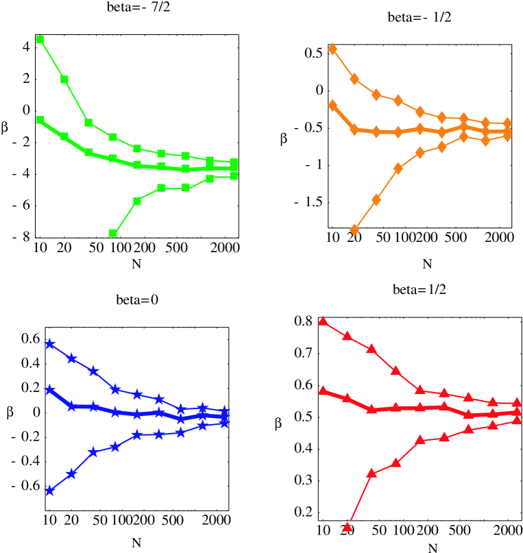
Figure 10: Median (thick line) and first and third quartiles (thin lines) for the distribution of $\langle\beta\rangle$ values determined by Eq. (10), from simulated proper motion samples, as a function of sample size (per bin) and for several values of true $\beta_{\star}$ for the underlying star cluster. The asymmetric width of the confidence bands reflects the asymmetric nature of the anisotropy parameter $\beta$. For small samples Eq. (10) allows unphysical derived values for $\beta$. Note the drift of the median as a function of $N$ which also reflects the fact that the pdf of $\hat{}\beta$ has inherited that of $\beta$, with both skewed towards negative values. See Eq. ( 23) and Fig. (11). The rather slow convergence of the estimator as a function of the number of stars for models with more negative $\beta$ is striking; this follows indirectly from Eq. (23) which has no well-defined moments.

Figure 11: Left Panel: Theoretical $\beta$ probability distribution (pdf) for $\beta_{\star}=1/2,-1/2\cdots-9/2$ as labelled. These distributions are very skewed, and their means and standard deviations are ill-defined. Right Panel: Monte Carlo estimate of the probability distribution of $\hat{}\beta$ for models corresponding to $\beta_{\star}=1/2,0,-1/2$ and $-7/2$. The distributions result from applying Eq. (10) to the values of $\langle v_{R}^{2}\rangle$ and $\langle v_{T}^{2}\rangle$ obtained for many random realizations of 20 stars from the respective star cluster models.

We generate $N$ stars sampled regularly in radius with a cumulative mass profile corresponding to Eq. (15). These are also required to obey Eq. (16), i.e. the number of stars at radius $r$ within ${{\rm d}{r}}$ with radial velocity $v_{r}$ within ${{\rm d}{v}}_{r}$ and tangential velocity $v_{t}$ within ${{\rm d}{v}}_{t}$ is given by

$${{\rm d}{N}}=8\pi^{2}\,r^{2}v_{t}\,f({\textstyle{\frac{1}{2}}}(v_{r}^{2}+v_{t}^{2})-\psi(r),rv_{t}){{\rm d}{r}}{{\rm d}{v}}_{t}{{\rm d}{v}}_{r}\,.$$ (21)

Given a triplet $(r,v_{r},v_{t})$, we generate a random position vector ${\bf{r}}=r\{\cos(\theta)\cos(\phi),\cos(\theta)\sin(\phi),\sin(\theta)\}$ where $z$ is along the line-of-sight as before, $\phi$ is a random number uniform in $[0,2\pi[$ and $\sin(\theta)$ is a random number uniform in $[-1,1[$. We also construct $v_{\theta}=v_{t}\cos(\chi)$ and $v_{\phi}=v_{t}\sin(\chi)$ where $\chi$ is a random number uniform in $[0,2\pi[$. The velocity vector then reads ${\bf{v}}=v_{r}{\bf{e_{r}}}+v_{\theta}{\bf{e_{\theta}}}+v_{\phi}{\bf{e_{\phi}}}$. It is then straightforward to project the components of ${\bf{r}}$ and ${\bf{v}}$ onto the plane of the sky.

Fig. (7) displays sky projections of the proper motion vectors of 250 stars drawn from $\beta_{\star}=1/2$ and $-1/2$ clusters, respectively. The length of each arrow is proportional to the magnitude of the projected proper motion. The figure shows that a radially anisotropic cluster is readily recognized by the many stars with radial proper motions: intrinsically radial orbits remain radial when projected onto the sky, and the number of radial proper motions is a good indicator of the number of radial orbits. By contrast, intrinsically tangential orbits may appear tangential or radial in the sky plane, depending on the orientation of their orbital planes. Correspondingly, the projection of the tangentially anisotropic cluster in Fig. (7), while showing fewer radial and more tangential proper motion vectors, still contains a significant number of the former. Therefore, tangentially anisotropic clusters are more difficult to recognize and discriminate from each other in terms of their apparent proper motion distributions. Once the model is sufficiently tangential, the ratio of radial to tangential proper motions is largely determined by the projection rather than by the intrinsic anisotropy.

4.3 Anisotropy estimators

From the Monte Carlo sample of stars we can estimate the previously used anisotropy indicators $\gamma_{TR}$, and $\langle\beta\rangle$ (Eq. (10) ). The histograms of the estimated $\gamma_{TR}$ in Fig. (8) confirm the above discussion quantitatively: (i) They show that radially anisotropic models are more easily recognized by their proper motion anisotropy than tangentially anisotropic models. Nonetheless, strongly tangentially anisotropic clusters are recognizable in terms of their many stars with $\gamma_{TR}$ near +1. (ii) The distribution of $\gamma_{TR}$ is slightly skewed towards positive values even for near-isotropic clusters. (iii) The histograms are always bimodal, i.e., have peaks near $\gamma_{TR}=\pm 1$. This is also recognizable in the data; cf. the bottom right panel of Fig. (5).

These histograms are discrete realizations of the probability distribution for $\gamma_{TR}$, and this in turn derives from the marginal probability distribution for the intrinsic quantity $\gamma_{tr}={(v_{t}^{2}-v_{r}^{2})}/{(v_{r}^{2}+v_{t}^{2})}$, i.e., the number of stars with $\gamma_{tr}$ in a small interval ${\rm d}\gamma_{tr}$. Once the distribution function is known this is straightforward to compute:

$${\rm pdf}(\gamma_{tr}){\rm d}\gamma_{tr}\propto\left\{\int f\left(\varepsilon(v_{r}[v_{t},\gamma_{tr}],v_{t}),rv_{t}\right)\frac{\partial v_{r}}{\partial\gamma_{tr}}\,v_{t}\,{{\rm d}{v}}_{t}\right\}\,{\rm d}\gamma_{tr}\,,$$

which yields (after normalization)

$${\rm pdf}(\gamma_{tr}){\rm d}\gamma_{tr}={\frac{n!(\sqrt{1+\gamma_{tr}})^{2n-1}}{\pi\,(2n-1)!!\sqrt{1-{\gamma_{tr}}}}}{\rm d}\gamma_{tr}\quad{\rm where}\quad(n)!!=n(n-2)(n-4)\cdots 1\,.$$ (22)

This pdf is illustrated in Fig. (9); it is strongly non-Gaussian and skewed for both $n>0$ and for an isotropic cluster. The reason why the isotropic curve is not symmetric is because we have defined $\gamma_{tr}$ in terms of the total $v_{t}^{2}$ on the sphere rather than one half that. The main point of this diagram is the non-uniform and sometimes bimodal shape of the distribution. The distribution of the observed $\gamma_{TR}$ pdf after projection is also shown in in Fig. (9) as a histogram for 5000 stars. Relative to the intrinsic pdf the number of (projected) radial orbits has been boosted, as discussed above; the distribution is now always bimodal. Thus in diagrams like Fig. ( 6) we should expect to always find an overabundance of stars near $\gamma_{TR}=\pm 1$ compared to values near $\gamma_{TR}\simeq 0$, with the ratio $N(\gamma_{TR}\mathrel{\hbox to0.0pt{\lower 3.0pt\hbox{$\mathchar 536\relax$}\hss}\raise 2.0pt\hbox{$\mathchar 316\relax$}}1)/N(\gamma_{TR}\mathrel{\hbox to0.0pt{\lower 3.0pt\hbox{$\mathchar 536\relax$}\hss}\raise 2.0pt\hbox{$\mathchar 318\relax$}}-1)$ containing the information about anisotropy.

Fig. (10) shows the median and first and third quartiles for the distribution of $\langle\beta\rangle$ values determined by Eq. (10) from simulated proper motion samples, as a function of sample size and for several values of true $\beta_{\star}$ for the underlying star cluster. These confidence bands are especially wide for negative values of $\beta_{\star}$ because it is a very asymmetric indicator of anisotropy. Indeed the marginal propability distribution for the $\beta$ values as determined from individual stellar velocities is given by (following the derivation of Eq. (22))

$$pdf(\beta){{\rm d}{\beta}}={\frac{\sqrt{2}\,2^{2n}\,n!(\sqrt{1-\beta})^{2n-1}}{\pi\,(2n-1)!!{(3-2\beta)^{n+1}}}}{{\rm d}{\beta}}\,.$$ (23)

This pdf is illustrated on the left panel of Fig. (11). Eq. ( 23) does not have any moments (i.e. the pdf does not fall off fast enough as a function of $\beta$ to allow for, say the mean and the variance to be computed). This implies that any estimator for its central value will be unreliable. The pdf for $\langle\beta\rangle$ estimated via Monte Carlo simulations, has inherited these asymmetries; see the right panel of Fig. ( 11). Because of the observed skewness we expect the mean and the median to overestimate the anisotropy, especially for more negative $\beta_{\star}$ models, as was indeed seen in Fig. (10).

We are now in a position to discuss the inferred anisotropies of the Galactic Centre star cluster (Fig. (5) and Table 2) in more detail. Comparing with the distributions in Fig. (9), the evidence for radial anisotropy in the central 0.”8 rests on the absence of stars with $\gamma_{TR}\simeq 1$, and the case for the tangential anisotropy of the HeI stars on the absence of stars with $\gamma_{TR}\simeq-1$. Based on the Monte Carlo models the evidence for anisotropy of the orbits is fairly solid. With larger proper motion samples, it may be best to compare with these distributions directly to estimate the anisotropy. The values for $\beta$ estimated from Eq. (10), on the other hand, are quite uncertain. With this estimator being a quotient of observable dispersions, its distributions are very broad (Fig. (11)). The Monte Carlo simulations indicate that a sample of 500 stars with $v/\sigma(v)$ greater than 3 will be required in order to determine even $\beta_{\star}=1/2$ to an accuracy of $\pm 0.2$.

In summary, the number of observed stars and the quality of the derived velocities is already sufficient to state with some certainty that anisotropies in the orbits of (early type) stars are indeed present. To be consistent with the observed distribution of $\gamma_{TR},$ the model clusters (assuming sphericity and cylindrical symmetry of the velocity ellipsoid) require fairly strong radial anisotropy at small radii, and tangential anisotropy for larger radii. However, the data are not yet suited to place accurate quantitative constraints on the anisotropy parameter $\beta$ and its radial dependence.

5 Global Rotation of the Early Type Cluster

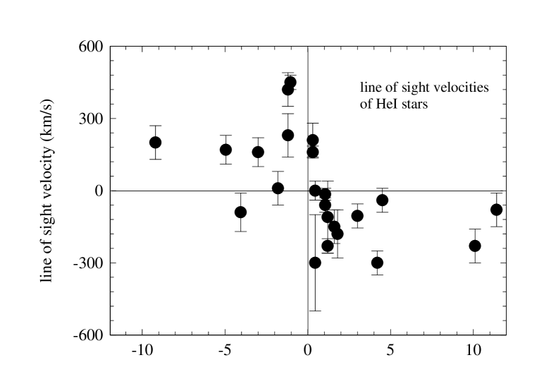
Figure 12: Line of sight velocities of all HeI stars in Table 1, as a function of Dec-offset from SgrA*. Error bars a $\pm 1\sigma$.

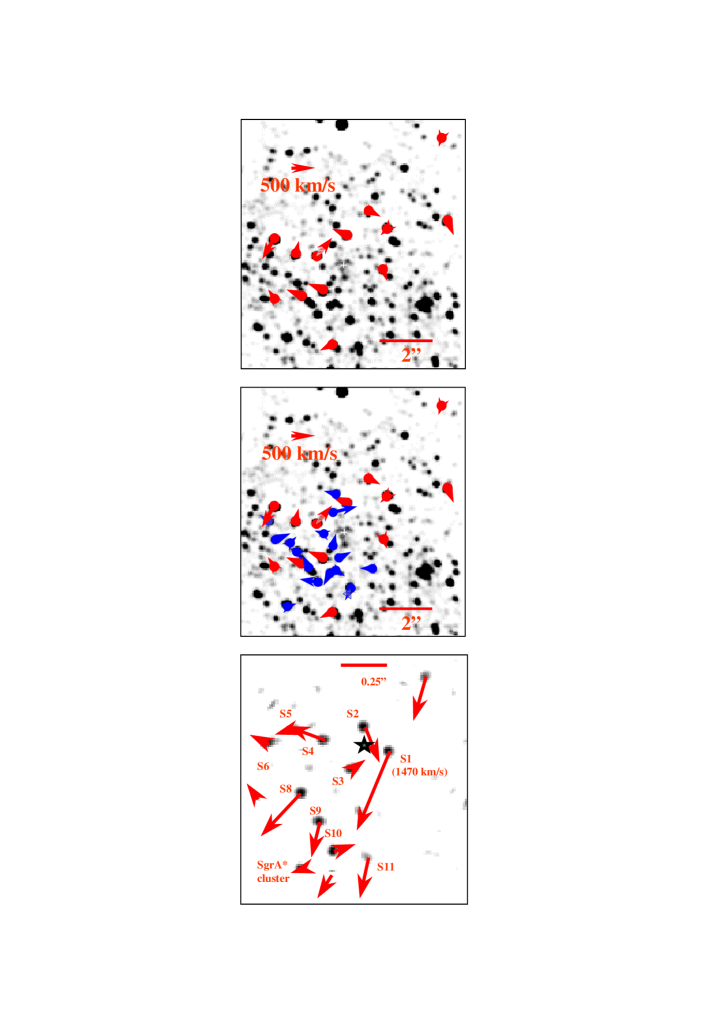
Figure 13: Proper motion vectors on K-band images of the central star cluster. North is up and East is to the left. Top: proper motion vectors of all HeI stars with three velocities, overlayed on a grey scale SHARP map at $0.15``$ resolution. The length and direction of each arrow denotes the magnitude and direction of the proper motion for each star. For comparison a 500 km/s motion (for $R_{{\sun}}=8.0{{\rm kpc}}$) is shown in the upper left. To indicate the uncertainties in direction for the best stars, a shaded cone is shown for IRS 16C. The white cross denotes the location of SgrA*. The middle panel shows in addition the vectors for all stars in the IRS 16 complex that have K-magnitude $\leq 13$. This criterion likely selects primarily early type stars. Proper motion vectors within $\approx{}0.7``$ of SgrA* (the ‘SgrA* cluster‘), overlayed on the 0.05“ resolution K-band map of Ghez et al. (1998) are given in the bottom panel. The asterisk marks the position of SgrA*. The $1\sigma$ positional uncertainty of the radio source on the infrared map is between $\pm$10 and $\pm$30 milli-arseconds (1$\sigma$). The identifications of the sources (S1-S11, Table 1) are given. The length of the proper motion of S1 corresponds to 1470 km/s for $R_{{\sun}}=8.0{{{\rm kpc}}}$.

As a group, the early type stars (= the starburst component) exhibit a well-defined overall angular momentum. The line-of-sight velocities of the 29 emission line stars follow a rotation pattern: blue-shifted radial velocities north, and red-shifted velocities south of the dynamic centre ( Fig. (12)). The apparent rotation axis is approximately east-west, within $\pm$20^∘. The early type stars thus are in a counter-rotation with respect to general Galactic rotation, the latter showing blue-shifted material south and red-shifted material north of the Galactic centre. The rotation is fast (average $\approx$150 km/s) and is consistent with a Keplerian boundary for a 2 to 3 million solar mass central mass (Fig. (12)). Our results confirm and improve the earlier conclusions of Genzel et al. (1996). Note that the late type stars also show an overall rotation, but that is slow (few tens of km/s) and consistent with Galactic rotation (McGinn et al. 1989, Sellgren et al. 1990, Haller et al. 1996, Genzel et al. 1996).

Eckart and Genzel (1996) have argued that the HeI stars also show a coherent pattern in their proper motions. Such a pattern is now confidently detected in the data (Fig. (13)). It is the origin for much of the tangential anisotropy discussed above. 11 of the 13 proper motion vectors for the emission line stars display a clockwise pattern, with only IRS16 NE and IRS 16NW moving counter-clockwise. A number of authors have argued that most of the members of the IRS16 complex (located between SgrA* and 4” east of it, and between 3.5” south of SgrA* and 1.5” north of it) belong to the early type cluster, with the HeI stars just being a sub-sample of the brightest emission line objects. This assertion is confirmed as well. Most of the brighter stars in the IRS16 complex (m${}_{{K}}\leq$13) show a clock-wise streaming pattern (Fig. (13) middle panel). In Fig. (13) (bottom panel) we overlay the proper motions vectors of Table 1 on the 0.05” resolution K-band Ghez et al. (1998) image of the SgrA* cluster. The preference of stars to be on radial/highly elliptical orbits that was discussed in the last section can be checked here from a graphical representation. Fig. (13) also suggests that the majority of stars in the SgrA* cluster have a similar projection of angular momentum along the line-of-sight, L_z, as the much brighter HeI stars and the IRS 16 cluster members. Speckle spectrophotometry (Genzel et al. 1997) and very recent high resolution VLT spectroscopy (Eckart et al. 1999) show that the brighter members of the SgrA* cluster lack 2.3-2.5$\mu$ m CO overtone absorption features and thus are clearly not late type stars. They are probably early type stars. If they are on the main sequence they would be of type B0 to B2. The SgrA* cluster members thus are probably part of the early type star cluster but are on plunging, radial or very elliptical orbits. The only alternative explanation of the observed radial anisotropies and net angular momentum is that the SgrA* cluster stars are rotating as a group, like the HeI stars, but with a rotation axis lying in or near the plane of the sky. While this explanation seems relatively implausible, measurements of proper motion curvature and radial velocities are required to make a decisive test.

However, the early type cluster cannot simply be modeled as an inclined, rotating thin disk. The fit of the best Keplerian disk model (inclination 40^o , v_rot=200 r^-0.5) to the HeI star velocities is poor. There are no HeI stars seen at Galactocentric radii greater than ~ 12”. Because the HeI stars should be phase-mixed along their orbits (§2.2), a better description of their distribution, and perhaps the entire early type cluster, probably is a dynamically hot and geometrically thick, rotating torus at radii from 1” to 10” (0.039 to 0.39 pc).

Most of the stars in the torus will have a fairly large angular momentum L and approximately the same sign of L_z. In the distribution of different L’s there is a small fraction of stars, however, with much smaller L and still the same sign(L_z). This sub-population is necessarily small and may thus not contain very massive stars. The low-L stars are able to pass much closer to SgrA* than the majority of the early type star cluster. In our interpretation, it is these stars on largely radial, plunging orbits that make up the SgrA* cluster. As the bright, more massive stars are on average at larger distances from SgrA*, it is possible to detect fairly easily this central sub-sample of fainter, fast moving stars. One would expect to find the same types of stars also at larger radii from SgrA*. However, the present proper motion data sets are biased against such fainter stars because of the presence of the brighter early type stars (especially the IRS 16 cluster) and of late type stars at yet larger true radii.

In summary of this section, we conclude that the majority of the HeI emission line stars and the bright (early type) stars in the IRS 16 cluster show a coherent clockwise and counter-Galactic rotation. Their circular (tangential) velocities dominate over their radial velocities. The young stars are arranged in a thick torus of mean radius $\approx$0.2 pc. This torus was presumably first formed $\approx$7 to 9 million years ago when one or several infalling, tidally disrupted clouds collided and were highly compressed. This lead to an episode of active star formation in the central parsec. From the presence of bright AGB stars in the same region (Krabbe et al. 1995, Genzel et al. 1996, Blum, Sellgren and dePoy 1996) it is likely that there were other such phases of active star formation in the more distant past (a few 10² million years ago).

6 Projected mass estimator and Anisotropy.

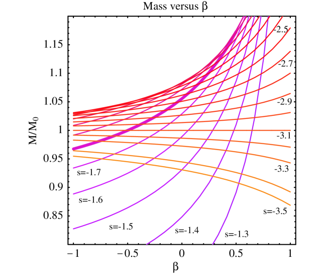
Figure 14: Leonard-Merritt mass estimates (in units of the true underlying mass) as a function of $\beta$ for different power law slopes of clusters as labelled (the thicker curve corresponds to $\rho\propto r^{-1.8}$). Note that for all power law clusters but that corresponding to $\rho\propto r^{-3}$, the mass estimate is typically biased and gives an overestimate or underestimate of the real mass. In particular note that the Bahcall Tremaine estimate (corresponding to $\beta=0$) is also offset for all slopes but $3$ and $1.62$. For instance for $\beta=0$ and $\rho\propto r^{-1.8}$, the relative mass discrepency reads $M_{{LM}}/M_{0}\approx 1.05$ but for $\beta=-5$ it reaches $\approx 0.89$ while a purely radial cluster would lead to an overestimation of 60 % as shown in Table 3. In practice our estimate of the mass of the black hole should be rescaled downward by about 5-10 % to account for this bias in the relevant radial range.

Table 3. Correction factor ${M_{{\rm LM}}}/{M_{0}}$ for LM mass estimator versus $\beta$ (horizontally) and $s$ (vertically). Note the steep rise near $\beta=1$ for shallower density profiles. The function (${M_{{\rm LM}}}/{M_{0}})(\beta,s)$ is illustrated in Fig. (14) $s\setminus\beta$ -5 -4 -3 -2 -1 0 0.25 0.5 0.75 1 -1.2 0.43 0.43 0.44 0.46 0.49 0.57 0.62 0.71 0.93 2.3 -1.4 0.67 0.67 0.69 0.71 0.75 0.85 0.91 1. 1.2 2. -1.5 0.74 0.75 0.77 0.79 0.83 0.93 0.99 1.1 1.3 1.9 -1.6 0.81 0.81 0.83 0.85 0.89 0.99 1. 1.1 1.3 1.8 -1.7 0.85 0.86 0.88 0.9 0.93 1. 1.1 1.2 1.3 1.7 -1.8 0.89 0.9 0.91 0.93 0.97 1.1 1.1 1.2 1.3 1.6 -1.9 0.92 0.93 0.94 0.96 0.99 1.1 1.1 1.2 1.3 1.5 -2. 0.94 0.95 0.96 0.98 1. 1.1 1.1 1.2 1.3 1.4 -2.2 0.97 0.98 0.99 1. 1. 1.1 1.1 1.1 1.2 1.3 -2.4 0.99 1. 1. 1. 1. 1.1 1.1 1.1 1.2 1.2 -2.5 1. 1. 1. 1. 1. 1.1 1.1 1.1 1.1 1.2 -2.6 1. 1. 1. 1. 1. 1.1 1.1 1.1 1.1 1.1 -2.8 1. 1. 1. 1. 1. 1. 1. 1. 1. 1.1 -3. 1. 1. 1. 1. 1. 1. 1. 1. 1. 1. -3.5 0.98 0.98 0.98 0.97 0.95 0.93 0.92 0.91 0.89 0.87

Leonard and Merritt (1989) have shown that an anisotropy-independent, projected mass estimator can be constructed from radially complete proper motion data. Starting from the Jeans equation for a spherically symmetric, non-rotating system,

$$GM(r)=-r\sigma_{{r}}^{{2}}\{{{\rm d}{\log}}n(r)/{{\rm d}{\log}}r+{{\rm d}{\log}}\sigma_{{r}}^{{2}}/{{\rm d}{\log}}r+2(1-\sigma_{{t}}^{{2}}/\sigma_{{r}}^{{2}})\}\quad,$$ (24)

one can construct the spatially averaged, stellar tracer density ($n(r)$) weighted expectation value $G\langle M(r)\rangle$. This estimator, henceforth referred to as the Leonard-Merritt (LM) estimator, is independent of any assumptions about anisotropy,

$$G\langle M(r)\rangle_{{LM}}=\langle r(2\sigma_{{r}}^{{2}}+2\sigma_{{t}}^{{2}})\rangle=(16/3\pi)\{2\langle R\sigma_{{R}}^{{2}}\rangle+\langle R\sigma_{{T}}^{{2}}\rangle)\quad.$$ (25)

Table 2 lists the LM-estimator obtained from 95 proper motion stars within $5^{\prime\prime}$ of SgrA*. The estimated mass is $2.9\pm 0.4\times 10^{{6}}M_{\sun}$. It is quite insensitive to the weighting scheme of the data. We also list LM-estimates for different projected annuli (although this is formally not appropriate, see below).

For comparison, the Bahcall-Tremaine (1981, BT) estimator for an isotropic cluster around a point mass gives a mass of $3.1\pm 0.3\times 10^{{6}}M_{\sun}$ for the 2x95 proper motions within $R=5^{\prime\prime}$ (Table 2). For purely radial orbits the mass would be twice as large. Note however that formally the BT estimator is defined for radial velocities only and as such the application to proper motions is inappropriate. The virial theorem mass estimate (VT) of the same data gives $2.5-2.6\times 10^{{6}}M_{\sun}$ (Table 2, see Bahcall and Tremaine 1981, or Genzel et al. 1996 for a discussion). The BT estimator requires prior knowledge of the orbit structure. In the region outside 3” from SgrA* where from our proper motion analysis the orbit structure is approximately isotropic, the agreement between all three estimators is fair (at somewhat more than $1\sigma$).

6.1 Correction for the Leonard-Merritt mass estimate

Unfortunately, the Leonard-Merritt mass estimate assumes that the cluster is of finite mass and that we have access to the full radial extent of the cluster. Here the density profile behaves roughly as a power law over the finite range of radii for which data is available. For such a mass model in a Keplerian potential the implementation of Leonard-Merritt mass estimate on concentric rings yields a biased (systematically offset) measure of the mass. Indeed the derivation of this estimator involves an integration by part of integrals of the form

$$\int\limits_{0}^{\infty}r^{4}\frac{{\rm d}\rho\sigma^{2}(r)}{{\rm d}r}{\rm d}r=-4\int\limits_{0}^{\infty}\rho(r)r^{3}\sigma^{2}(r){\rm d}r+\left[\rho(r)r^{4}\sigma^{2}(r)\right]_{0}^{\infty}$$ (26)

For finite mass systems the second term of the right hand side of Eq. (26) vanishes. In the context of the Galactic centre we still compute

$${\int_{r_{1}}^{r_{2}}\rho(r)r^{3}\sigma^{2}(r){\rm d}r}/{\int_{r_{1}}^{r_{2}}\rho(r)r^{2}\sigma^{2}(r){\rm d}r}$$ (27)

over a finite radial range $r_{1},r_{2}$ and even though both numerator and denominator diverge as $r_{1}\rightarrow 0$ and $r_{1}\rightarrow\infty$, the ratio is well defined and equals the value corresponding to finite $r_{1}$ and $r_{2}$. On the other hand

$$\left[\rho(r)r^{4}\sigma^{2}(r)\right]_{r_{1}}^{r_{2}}/{\int_{r_{1}}^{r_{2}}\rho(r)r^{2}\sigma^{2}(r){\rm d}r}$$ (28)

is also finite but non zero except for $s=-3$. As a consequence the ratio $M_{{\rm LM}}/M_{0}$ will typically be a function of $\beta$ and $s$, the slope of the local power law corresponding to the range for which data is available. A straightfoward calculation yields

$$\frac{M_{{\rm LM}}}{M_{0}}={\frac{{2^{4+s}}\,{\Gamma}({{-s}/{2}})\,\left(\left(3-s\right)\,\left(1-s-\beta\right)\,{\Gamma}(-s)-{\Gamma}(2-s)\right)}{3\,{\sqrt{\pi}}\,\left(1-s-2\,\beta\right)\,{\Gamma}({{-s/2-1/2}{}})\,{\Gamma}({{1/2-s/2}{}})\,{\Gamma}({{3/2-s/2}{}})}}$$ (29)

Relevant relative mass estimates versus $\beta$ for different power law index are shown in Fig. (14). In practice Eq. (29) is used to correct for the offset in the measured $M_{{\rm LM}}$. Table 3 gives a few values relevant for the Galactic centre.

Note that ${M_{{\rm LM}}}={M_{0}}$ for $\beta=0$ when $s$ is $-3$ or the root of

$$16\,{}{\Gamma}({{s}/{2}})\,\left(\left(1-s\right)\,\left(3-s\right)\,{}{\Gamma}(s)-{}{\Gamma}(2-s)\right)=3\,{2^{1-s}}\,{\sqrt{\pi}}\,{}{\Gamma}({{-s/2-1/2}{}})\,{{{}{\Gamma}({{3/2-s/2}{}})}^{2}}$$ (30)

which yields $s\approx-1.62$. More generally there is a non trivial curve (i.e. which differs from ${s=-3}$) corresponding to $M_{{\rm LM}}/M_{0}=1$ in the $(\beta,s)$ plane.

We conclude that the LM-estimator is not independent of $\beta$ or $s$ when applied to truncated data set even though each shell yields the same mass estimate for a Keplerian potential. We do need to estimate $\beta$ and $s$ independently to correct for the offset. Since $\beta$ varies with radius for the Galactic centre the correction will affect the mass profile.

The mass estimators are derived by averaging over the entire star cluster, while the observed stars in the Galactic centre are presumably part of a more extended stellar system. To test for possible systematic effects, we have therefore also carried out Monte Carlo simulations for the LM-estimator. Again, as in Section 4.2, we have used a power law distribution of tracer stars with $n\propto r^{-2.5}$ as for the kinematically measured stars. The left panel of Fig. (15) shows the median and quartiles of the distribution of $M_{LM}$ values derived for many star cluster realizations, as a function of sample size and for $\beta_{\star}=0.5,0,-0.5$, and $-3.5$. The true mass of the central black hole that dominates the potential of these clusters is $M=1$. The right panel of Fig. (15) shows, for $N=800$ stars, the effect of estimating the central mass from five concentric annuli aranged linearly as a function of radius. Note that the mass profile is indeed flat (within the statistical uncertainties) as expected for a Keplerian potential and offset by the amount predicted by Eq. (29).

These simulations suggest that applying the LM-estimator to a central sub-volume of the actual star cluster around the black hole gives the correct hole mass if the distribution of orbits is strongly tangential, independent of power law slope (all radial shells should then be independently sufficient). For isotropic and radially anisotropic orbit distributions and power law slopes near -2 the LM-estimator gives somewhat biased (too high) values for the central mass. The value of $M=2.9\times 10^{6}M_{\odot}$ derived for the central mass from all stars inside 5” (an approximately overall isotropic sample) thus is likely systematically high by about $5-10\%$.

Figure 15: Left: Median and quartiles for the distribution of values for the mass estimator $M_{LM}$ (Eq. (10)) from simulated proper motion samples, as a function of sample size and for several underlying anisotropy values $\beta_{\star}=0.5,0,-0.5,-3.5$ of the simulated star cluster. The true central mass is unity and the offset induced by the LM estimation is clearly visible there and in accordance with the theoretical prediction from Table (6). Mass determinations reliable at the 10% level require samples of at least 40, 35, 25, and 15 stars for $\beta_{\star}=0.5,0,-0.5,-3.5$. Right: Central mass estimates $M_{LM}$ derived in five annuli on the sky for a total number of 800 stars. anisotropy values are $\beta_{\star}=0.5,-0.5,$ and $-3.5$, as labelled (plain,dash-dot,long dash,dash) corresponding to (triangle,star,diamond,square).

6.2 Estimate of the Sun-Galactic centre distance R_☉

The expectation values of the first moments of the projected velocity dispersions are related to each other through their mutual dependence on the intrinsic radial and tangential velocity dispersions. One can write

$$\langle R\sigma_{{z}}^{{2}}\rangle=(1/3)\langle R\sigma_{{R}}^{{2}}\rangle+(2/3)\langle R\sigma_{{T}}^{{2}}\rangle\quad.$$ (31)

The z-velocity is determined directly through the Doppler shifts of the stars. The R- and T-velocities depend on the assumed Sun-Galactic centre distance R_☉. For a spatially and kinematically spherical system it is therefore possible to derive the distance to the Galactic centre from equation (31), without any prior assumptions on the anisotropy. The relationship is

$$(R_{{\sun}}/8{{\rm kpc}})=(\langle R\sigma_{{z}}^{{2}}\rangle_{{8}}/\{1/3\langle R\sigma_{{R}}^{{2}}\rangle_{{8}}+2/3\langle R\sigma_{{T}}^{{2}}\rangle_{{8}}\})^{{0.5}}\quad.$$ (32)

Here $\langle$ $\rangle_{{8}}$ refers to the values calculated under the assumption that the Galactic centre distance is 8.0 kpc, as assumed for the proper motions in Table 1. Taking only those 32 stars for which we have all three velocity components we find $R_{{\sun}}=8.95\pm 1.6{{{\rm kpc}}}$. Taking all 104 proper motion stars within $R\leq 8.8^{\prime\prime}$ and all 71 stars with z-velocities within the same projected radius we find R_☉=8.2$\pm$0.9 kpc. The specific moment analysis in equation (32) as applied to these samples is appropriate if the motions are completely dominated by a central point mass. In that case $R\sigma^{{2}}\approx$const and data points at different R (but the same quality) are appropriately given the same weight. In the Galactic centre the mass distribution is a sum of a central point mass and a near-isothermal stellar cluster of velocity dispersion $\sigma_{{0}}$=50 to 55 km/s derived from the stellar velocities outside the sphere of influence of the black hole (Genzel et al. 1996). It may thus be more appropriate to subtract $\sigma_{{0}}^{{2}}$ before computing the expectation values in equations (26) and (27). In that case we obtain $R_{{\sun}}=7.9\pm 0.85{{\rm kpc}}$. The difference between these two last estimates arises since the line-of-sight velocity data are biased to a larger $\langle R\rangle$ than the proper motions so that the effect of removing $\sigma_{{0}}$ has a larger impact on the z-velocities. This differentially decreases slightly the distance estimate relative to that obtained for $\sigma_{{0}}=0$. All errors do not contain a possible systematic term from deviations from spherical symmetry.

Our analysis is in excellent agreement with other recent estimates for the Galactic centre distance which range between 7.2 and 9.0 kpc with a best weighted average of 8.0$\pm$0.5 kpc (see the review of Reid 1993). The statistical uncertainty of our estimate rivals the best other methods available for determining R_☉: cluster parallaxes through H₂O maser proper motions, global modeling of the Galaxy, globular cluster dynamics, RR-Lyrae stars, Cepheids, planetary nebulae and OB stars in HII regions (Reid 1993) and clump giant stars (Paczynski & Stanek 1998).

7 Jeans modeling of the central mass distribution

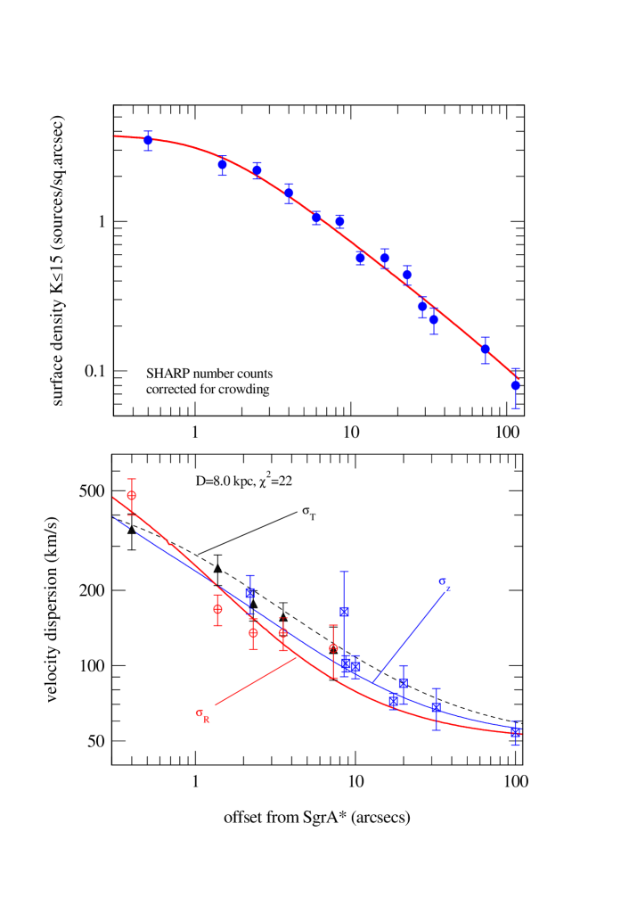
Figure 16: Surface density and velocity dispersions as a function of projected separation from SgrA*, along with the best fitting anisotropic Jeans model described in section 7. The observed m(K)$\leq$15 surface density counts and their 1$\sigma$ uncertainties are shown in the left inset (see also Table 4). These counts come from Schmitt (1995) and have been corrected for the effects of crowding and bright stars. The continuous curve is the model of Eq. (33) with the parameters in Table 5, integrated along the line of sight as described in equations  ( 5) and  (6). The right inset shows observations of the projected tangential velocity dispersionss (T: triangles, this paper, Table 2), projected radial velocity dispersions (R: circles, this paper, Table 2) and line of sight velocity dispersions (z: rectangles with crosses, Table 4). The data for the line of sight dispersions come from this paper (HeI stars), from Genzel et al. (1996), Haller et al. (1996), Lindqvist et al. (1992), Sellgren et al. (1990) and McGinn et al. (1989). The best anisotropic Jeans model integrated along the line of sight (Table 5) gives the black, thin dashed curve for the projected tangential (T) data points, the red, thick continuous curve for the projected radial ( R ) data points and the blue, thin continuous curve for the line-of-sight (z) data points. The model assumes a distance of 8 kpc and gives a total $\chi^{{2}}$ of 21.6, or a reduced $\chi^{{2}}$/N of 0.83.

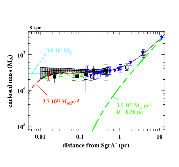
Figure 17: Mass distribution in the central 10 pc of the Galaxy obtained from stellar and gas dynamics (for $R_{{o}}=8.0{{{\rm kpc}}}$). The different data points (all with $\pm$1$\sigma$ uncertainties) are as follows. Bold ‘G’ denotes mass estimates from the ionized and neutral gas dynamics (Serabyn and Lacy 1985, Güsten et al. 1987, Lacy et al. 1991, Herbst et al. 1993, Roberts and Goss 1993). Rectangles with crosses and down-pointing triangles denote the isotropic mass modeling of Genzel et al. (1996, 1997), including Jeans modeling of stellar radial velocities (early and late type stars, filled down pointing triangles) and Bahcall-Tremaine estimators of the NTT proper motions until 1996 (open down pointing triangles). Open rectangles (with crosses) are Bahcall-Tremaine estimators of the line of sight velocity data only. Open up-pointing triangles are the Bahcall-Tremaine estimators of the 1995-1996 proper motion data of Ghez et al. (1998). The new anisotropy independent mass estimates from the present work are given as filled black rectangles (Leonard-Merritt estimators of the proper motions in (Table 1, Table 2) and as large black crosses connected by a continuous curve (Jeans model, Table 5). For comparison several model curves are shown. The green, thick dashed curve represents the mass model for the (visible) stellar cluster ($M/L(2\mu m)=2,r_{{\rm core}}=0.38{{\rm pc}}$, $\rho(r=0)=3.5\times 10^{{6}}M_{{\sun}}{{\rm pc}}^{{\ -3}}$). The light blue, continuous curve is the sum of this stellar cluster, plus a point mass of $3.0\times 10^{{6}}M_{{\sun}}$. The red, dashed curve is the sum of the visible stellar cluster, plus an $\alpha=5$ Plummer model ($\rho(r)=\rho(0)(1+(r/r_{{0}})^{{2}})^{{-\alpha/2}})$ of a dark cluster of central density $3.7\times 10^{{12}}M_{{\sun}}{{\rm pc}}^{{-3}}$ and $r_{{0}}=0.0058{{\rm pc}}$.

We have also carried out a full Jeans modeling of the data set, explicitly allowing for the anisotropy term in equation  (24). It is clear that the number of stars is still too small to unambiguously determine the radial profiles of anisotropy and mass for all different stellar components (and including rotation). Here we only give a simplified overall model which is consistent with all the data. Our model proceeds from a parameterized Ansatz for the different quantities, as described earlier in Genzel et al. (1996),

$$n(r)=2n_{{0}}/(\pi r_{{0}}\{1+(r/r_{{0}})^{{\alpha}_{r}}\}),\quad\sigma_{{r}}^{{2}}(r)=\sigma_{{r0}}^{{2}}(r/r_{{0}})^{{-2\alpha}_{\sigma r}}+\sigma_{{0}}^{{2}}\quad{\rm and}\quad\sigma_{{t}}^{{2}}(r)=\sigma_{{t0}}^{{2}}(r/r_{{0}})^{{-2\alpha}_{\sigma t}}+\sigma_{{0}}^{{2}}\quad.$$ (33)

To compare to the observed surface density distribution $\Sigma(R)$, and observed velocity dispersions $\sigma_{{z}}(R)$, $\sigma_{{R}}(R)$ and $\sigma_{{T}}(R)$ the expressions in equation  (33) were numerically integrated along the line of sight and weighted with the density distribution, as described in equations  (5) and  (6) . The data were averaged in annuli centered around SgrA* to yield 13 values for $\Sigma(R)$ between R=0.5 and 114”, 8 values for $\sigma_{{z}}(R)$ between R=2 and 100” and 5 values each for $\sigma_{{R}}(R)$ and $\sigma_{{T}}(R)$ between R=0.4 and 7.3”. Best fit values for the 8 parameters in the expressions above were then determined from a $\chi^{{2}}$ minimization. They are listed in Table 5. The surface density measurements come from number counts with the SHARP speckle camera to m(K)=15 and are corrected for crowding and incompleteness (Schmitt 1995). The data points and their statistical errors are listed in Table 4. The R- and T- velocity dispersion values are from Table 2. The line of sight velocity dispersions are listed in Table 4 as well. The two data points at R=2.2 and 8.5” are derived from the HeI star velocities in Table 1. In addition we have taken late type star velocity dispersions from Genzel et al. (1996) and references therein. The 13 surface density measurements in Table 4 constrain the 3 parameters of the density distribution given in expression Eq. (33) very well. Likewise the 18 velocity dispersion measurements also give good constraints on the 5 parameters of the dispersion expressions in Eq. (33).

Fig. (16) shows the surface density and velocity data, along with the best fit model whose parameters are given in Table 5. Table 5 also lists the best anisotropic mass model, along with the logarithmic gradients and the $\beta$ -anisotropy parameter that were used in the Jeans equation (Eq. (24 )) to derive that mass model.

8 Discussion and Conclusions

The connected black crosses in Fig. (17) depict the mass distribution obtained from the Jeans-model with anisotropy (and its (1$\sigma$) uncertainty). For comparison we also show the LM-mass estimators from Table 2, BT estimators for the z- and proper motions (this paper, Genzel et al. 1996, 1997, Ghez et al. 1998), the isotropic Jeans mass model of Genzel et al.(1996) and a few of the mass estimates determined from the gas motions (Guesten et al. 1987, Serabyn and Lacy 1985, Lacy et al. 1991, Herbst et al. 1993, Roberts et al. 1993). The mass inside of the innermost bin ($r=0.01{{\rm pc}}$) of our best Jeans model is $3.25\times 10^{{6}}M_{\sun}$. It is consistent with the Leonard-Merritt mass estimator of the entire proper motion sample inside $5^{\prime\prime},M_{{LM}}=2.9\pm 0.4\times 10^{{6}}M_{\sun}$ (Table 2, see also Section 6). When corrected for the bias discussed above that mass becomes about $2.6-2.8\times 10^{{6}}M_{\sun}$. Systematic effects and the method of modelling dominate the accuracy to which the central mass can be determined. In Fig. (17) we plot a central mass of $3.0\times 10^{6}M_{\sun}$. This value is a compromise between the bias-corrected LM-estimate and the Jeans estimate. Its overall (systematic plus statistical) uncertainty is $\pm 0.5\times 10^{6}M_{\sun}$. It is reassuring that the results of our simple anisotropic modeling and of previous isotropic models are in good agreement within the respective errors. Our results confirm that the mass distribution is flat between $0.01$ and $0.5{{\rm pc}}\/$.

Nonetheless, there are still significant uncertainties in this analysis.

(i) The parametric form of the model fitted to the data is not unique.

(ii) We have so far not distinguished between early and late type stars. Yet it is fairly clear that early and late type stars have different spatial distributions and kinematics (see Plate 1 in Genzel et al. 1996). In the Jeans analysis, we require the density distribution and kinematics of an equilibrium tracer population. The proper motions stars are heavily influenced by spatial selection biases; thus it is not appropriate to use their inferred number density distribution in the Jeans equation. Their role is to provide local velocity measurements for the population that they represent. The early-type stars contribute much to these kinematic measurements; if they are more centrally concentrated than the overall population measured by the SHARP number counts, this will have the effect of underestimating the central mass.

(iii) The version of the Jeans equation we have used in expression  (24) neglects rotation. Yet we have discussed above the strong evidence for coherent motion of the HeI star cluster. The late type stars have only a small overall rotation. Including rotation and distinguishing in the analysis between late and early type stars would thus be desirable (as in Genzel et al. 1996 for the isotropic case). Unfortunately this is not possible, because of the large number of free parameters (3 more for density distribution, approximately 8 more for velocity distribution) and the relatively poor constraints on a number of the parameters. There are no early type stars outside 11”, there are very few late type stars inside 5”and the accuracy of the proper motion R- and T-velocity dispersions is low if all proper motions without a stellar type identification are discarded. We have run models with explicit inclusion of rotation but found it to be overall a poorer fit than the models without rotation. To deliberately deemphasize the rotation signature of the HeI star cluster we have arbitrarily given the z-velocity dispersion value at $R=8.5^{\prime\prime}$ (Table 4) a low weight.

The central dark mass concentration is most likely a point mass. Any configuration other than a point mass must have a central density of $\rho(0)\geq 3.7\times 10^{{12}}M_{\sun}{{\rm pc}}^{{-3}}$and a core radius of $r_{{0}}\leq 5.8$ milli-parsec . For this estimate we have adopted a Plummer model with a density profile that decreases as $r^{{-5}}$ outside of the core radius. In a configuration with a point mass and the visible stellar cluster $(\rho_{{\ast}}(0)=3.5\times 10^{{6}}M_{\sun}{{\rm pc}}^{{-3}},\alpha=1.8,r_{{0}}=0.17{{\rm pc}}$) as the two main components of the mass distribution any additional mass within $\approx 0.2-0.5{{\rm pc}}$ of SgrA* must be less than $\approx 1\times 10^{{6}}M_{\sun}$, or 32% of the point mass. If one takes the LM-mass distribution instead (Table 2), that limit would be between $1.1$ and $2.2\times 10^{{6}}M_{\sun}.$ Backer (1996) has shown that the proper motion of SgrA* itself is $\leq 16{\rm km\,s}^{-1}$, or fifty to one hundred times smaller than the fast moving stars in its vicinity. Thus the mass enclosed within the radio size of SgrA* ($r\leq 1AU$) is $\geq 10^{{3}}$ or $\geq 10^{{5}}M_{\sun}$, depending on whether the radio source is in momentum or energy equilibrium with the fast moving stars (Genzel et al. 1997, Reid 1999). Even the more conservative of these two limits implies a central density in excess of $10^{{18}}M_{\sun}{{\rm pc}}^{{-3}}$.

Our results confirm and strengthen recent work on the central mass distribution (cf. Eckart and Genzel 1996, 1997, Genzel et al. 1997, Genzel and Eckart 1997 , Ghez et al. 1998). From these papers and from Maoz (1998) it appears that the most likely configuration of the central mass concentration is a massive, but currently inactive black hole. With the parameters given above any dark cluster of stellar remnants (neutron stars, stellar black holes), low luminosity stars (e.g. white dwarfs) or sub-stellar objects would have a lifetime less than $\approx{}10^{{7}}$ years. This is much smaller than the ages of most of the stars in the Galactic centre, requiring that we happen to observe the Galactic centre in a highly improbable, special period. In addition, the very steep outer density distribution of such a dark cluster implied by the mass distribution in Fig. (17) $(\rho\approx{}r^{{-\alpha}}$with $\alpha\geq 5)$ is inconsistent with any known observed dynamical system. It is also inconsistent with the results of physical models, including those of core-collapsed clusters (see the discussion of Genzel et al. 1997). Maoz (1998) points out that the only possible - albeit highly implausible - alternatives to a central black hole are a concentration of heavy bosons and a compact cluster of light $(\leq 0.005M_{\sun})$ ‘mini’-black holes.

Acknowledgements. We would like to thank David Merritt for making us aware of the mass estimators first laid out in his paper with Peter Leonard in 1989, as well as for comments on the present manuscript. We also appreciate the willingness of the ESO Director General and his staff to let us bring the SHARP camera to the NTT in 1997 and 1998. We thank Niranjan Thatte, Alfred Krabbe, Harald Kroker and the entire MPE-3D team for their help with the 3D observations on the ESO-MPG 2.2m and for developing the new data reduction tools necessary to analyse the data set presented here. We are also grateful to the NTT-team and especially to U.Weidenmann and H.Gemperlein for their interest and technical support of SHARP at the NTT. CP would like to thank E. Thiébaut for many valuable discussions. We thank Lowell Tacconi-Garman and Linda Tacconi for comments on and help with the manuscript. We are grateful to the referee for his valuable and helpful comments. Funding from the Swiss NF is gratefully acknowledged.

References

- [1] Allen, D.A., Hyland, A.R. and Hillier, D.J. 1990, MNRAS 244, 706
- [2] Backer, D.C. 1996, in Unsolved Problems of the Milky Way, eds. L.Blitz and P.Teuben, Proc. of IAU 169 (Kluwer:Dordrecht), 193
- [3] Bahcall, J.N. and Tremaine S.C. 1981, Ap.J. 244, 805
- [4] Blum, R.D., DePoy, D.L. and Sellgren, K. 1995b, Ap.J. 441, 603
- [5] Blum, R.D., Sellgren, K. and DePoy, D.L. 1995a, Ap.J. 440, L17
- [6] Blum, R.D., Sellgren, K. and DePoy, D.L. 1996, A.J. 112, 1988
- [7] Bower, G.C. and Backer, D.C. 1998, Ap.J. 496, L97
- [8] Christou, J.C. 1991, Experimental Astr. 2, 27
- [9] Eckart, A., Genzel, R., Krabbe, A., Hofmann, R., van der Werf, P.P. and Drapatz, S. 1992, NATURE 355, 526
- [10] Eckart, A. Genzel, R., Hofmann, R., Sams, B.J. and Tacconi-Garman, L.E. 1993, Ap.J. 407, L77
- [11] Eckart, A. , Genzel, R., Hofmann, R., Sams, B.J., Tacconi-Garman, L.E. and Cruzalebes, P. 1994, in ‘The Nuclei of Normal Galaxies’, eds. R.Genzel and A.I. Harris, NATO ASI Kluwer :Dordrecht), 305
- [12] Eckart, A. Genzel, R., Hofmann, R., Sams, B.J. and Tacconi-Garman, L.E. 1995, Ap.J. 445, L26
- [13] Eckart, A. and Genzel, R. 1996, NATURE 383, 415
- [14] Eckart, A. and Genzel, R. 1997, MNRAS 284, 576
- [15] Eckart, A., Ott, T. and Genzel, R. 1999, Astr.Ap. 352, L22
- [16] Genzel, R., Thatte, N., Krabbe, A., Kroker, H. and Tacconi-Garman, L.E. 1996, Ap.J.472, 153
- [17] Genzel, R., Eckart, A., Ott, T. and Eisenhauer, F. 1997, MNRAS 291, 219
- [18] Gerhard, O.E., 1991, MNRAS 250, 812
- [19] Ghez, A., Klein, B., Morris, M. and Becklin, E., 1998, Ap.J. 509, 678
- [20] Greenhill, L.J., Jiang, D.R., Moran, J.M., Reid, M.J., Lo, K.Y. and Claussen, M.J. 1995, Ap.J. 440, 619
- [21] Güsten R., Genzel, R., Wright, M.C.H., Jaffe, D.T., Stutzki, J. and Harris, A.I. 1987, Ap.J. 318, 124
- [22] Haller, J.W., Rieke, M.J., Rieke, G.H., Tamblyn, P., Close,L. and Melia,F. 1996, Ap.J. 456, 194
- [23] Heisler, J., Tremaine, S. and Bahcall, J.N. 1985, Ap.J. 298, 8
- [24] Herbst, T.M., Beckwith, S.V.W., Forrest, W.J. and Pipher, J.L. 1993, A.J.105,956
- [25] Hofmann, R., Blietz, M., Duhoux, P., Eckart, A., Krabbe, A. and Rotaciuc, V. 1993, in ‘Progress in Telescope and Instrumentation Technologies’, ed. M.H. Ulrich, ESO Report 42, 617
- [26] Kormendy, J. and Richstone, D. 1995, Ann.Rev.Astr.Ap.1995, 581
- [27] Krabbe, A. Genzel, R., Eckart, A., Najarro, F., Lutz, D. et al. 1995, Ap.J.Lett. 447, L95
- [28] Krabbe, A., Genzel, R., Drapatz, S. and Rotaciuc, V. 1991, Ap.J. 382, L19
- [29] Lacy, J.H., Achtermann, J.M. and Serabyn, E. 1991, Ap.J. 380, L71
- [30] Leonard, P.J.T. and Merritt, D. 1989, Ap.J. 339, 195
- [31] Libonate, S., Pipher, J.L., Forrest, W.J. and Ashby, M.L.N. 1995, Ap.J. 439, 202
- [32] Lindqvist, M., Habing, H. and Winnberg, A. 1992, Astr.Ap. 259, 118
- [33] Lo, K.Y., Shen, Z.-Q., Zhao, J.-H. and Ho, P.T.P. 1998, Ap.J. 508, L61
- [34] Maoz, E. 1998, Ap.J. 494, L131
- [35] McGinn, M.T., Sellgren K., Becklin, E.E. and Hall, D.N.B. 1989, Ap.J. 338, 824
- [36] Menten, K.M., Eckart, A., Reid, M.J. and Genzel, R. 1997, Ap.J. 475, L111
- [37] Myoshi, M., Moran, J.M., Hernstein, J., Greenhill, L., Nakai, N., Diamond, P. and Inoue, M. 1995, Nature 373, 127
- [38] Magorrian, J. et al. 1998, A.J. 115, 2285
- [39] Meynet, G., Maeder, A, Scahller, G., Schaerer, D. and Charbonnel, C. 1994, Astr.Ap.Suppl. 103, 97
- [40] Najarro, F., Hillier, D.J., Kudritzki, R.P., Krabbe, A., Lutz, D., Genzel, R., Drapatz, S. and Geballe, T.R. 1994, Astr.Ap.285, 573
- [41] Najarro, F., Krabbe, A., Genzel, R., Lutz, D., Kudritzki, R.P. and Hillier, D.J. 1997, Astr.Ap. 325, 700
- [42] Ott, T., Eckart, A. and Genzel, R. 1999, Ap.J. in press
- [43] Paczynski, B., Stanek, K.Z. 1998, ApJ 494, L219
- [44] Reid, M. 1993, Ann.Rev.Astr.Ap. 31, 345
- [45] Reid, M.J. 1999, in The Central Parsec, 1998 Tucson Galactic Center Wokshop, eds. H.Falcke, A.Cotera, W.Duschl, F.Melia and M.Rieke, ASP conf. Series, in press
- [46] Richstone, D. et al. 1998, NATURE 395, 14
- [47] Rieke, G.H. and Rieke, M.J. 1988, Ap.J. 330, L33
- [48] Roberts, D.A. and Goss, W.M. 1993, Ap.J.(Suppl.) 86, 133
- [49] Schmitt, J. 1995, Diploma Thesis, Ludwig-Maximilian University, Munich
- [50] Sellgren, K., McGinn, M.T., Becklin, E.E. and Hall, D.N.B. 1990, Ap.J. 359, 112
- [51] Serabyn, E. and Lacy, J.H 1985, Ap.J. 293, 445
- [52] Tamblyn, P., Rieke, G.H., Hanson, M.M., Close, L.M., McCarthy, D.W. and Rieke, M.J. 1996, Ap.J. 456, 206
- [53] Thatte, N., Weitzel, L., Cameron, M., Tacconi-Garman, L.E., Krabbe, A. and Genzel, R. 1995, SPIE conference proceedings, Ed.G.C.Holst 2224, 279
- [54] van der Hulst, J.M., Terlouw, J.P., Begeman, K., Zwitser, W. and Roeelfsema, P.R. 1992, in Astronomical Data Analysis Software and Systems I, eds. D.M.Worall, C.Biemesderfer and J.Barnes, ASP Conf.Ser. 25, 131
- [55] Weitzel, L., Krabbe, A. , Kroker, H., Thatte, N., Tacconi-Garman, L.E., Cameron, M. and Genzel, R. 1996, Astr.Ap.(Suppl.) 119, 531
- [56] Wollman, E.R., Geballe, T.R., Lacy, J.H., Townes, C.H. and Rank, D.M. 1977, Ap.J. 218, L103