Starburst-driven galactic winds: I. Energetics and intrinsic X-ray emission

Abstract

Starburst-driven galactic winds are responsible for the transport of mass, in particular metal enriched gas, and energy out of galaxies and into the inter-galactic medium. These outflows directly affect the chemical evolution of galaxies, and heat and enrich the inter-galactic and inter-cluster medium.

Currently several basic problems preclude quantitative measurements of the impact of galactic winds: the unknown filling factors of, in particular, the soft X-ray emitting gas prevents accurate measurements of densities, masses and energy content; multiphase temperature distributions of unknown complexity bias X-ray determined abundances; unknown amounts of energy and mass may reside in hard to observe $T\sim 10^{5}{\rm\thinspace K}$ and $T\sim 10^{7.5}{\rm\thinspace K}$ phases; and the relative balance of thermal vs. kinetic energy in galactic winds is not known.

In an effort to address these problems we have performed an extensive hydrodynamical parameter study of starburst-driven galactic winds, motivated by the latest observation data on the best-studied starburst galaxy M82. We study how the wind dynamics, morphology and X-ray emission depend on the host galaxy’s ISM distribution, starburst star formation history and strength, and presence and distribution of mass-loading by dense clouds. We also investigate and discuss the influence of finite numerical resolution on the results of these simulations.

We find that the soft X-ray emission from galactic winds comes from low filling factor ($\eta\mathrel{\hbox to0.0pt{\lower 3.0pt\hbox{$\sim$}\hss}\raise 2.0pt\hbox{$<$}}2$ per cent) gas, which contains only a small fraction ($\mathrel{\hbox to0.0pt{\lower 3.0pt\hbox{$\sim$}\hss}\raise 2.0pt\hbox{$<$}}10$ per cent) of the mass and energy of the wind, irrespective of whether the wind models are strongly mass-loaded or not. X-ray observations of galactic winds do not directly probe the gas that contains the majority of the energy, mass or metal-enriched gas in the outflow.

X-ray emission comes from a complex phase-continuum of gas, covering a wide range different temperatures and densities. No distinct phases, as are commonly assumed when fitting X-ray spectra, are seen in our models. Estimates of the properties of the hot gas in starburst galaxies based on fitting simple spectral models to existing X-ray spectra should be treated with extreme suspicion.

The majority of the thermal and kinetic energy of these winds is in a volume filling hot, $T\sim 10^{7}{\rm\thinspace K}$, component which is extremely difficult to probe observationally due to its low density and hence low emissivity. Most of the total energy is in the kinetic energy of this hot gas, a factor which must be taken into account when attempting to constrain wind energetics observationally. We also find that galactic winds are efficient at transporting large amounts of energy out of the host galaxy, in contrast to their inefficiency at transporting mass out of star-forming galaxies.

1 Introduction

Starbursts, episodes of intense star formation lasting $\mathrel{\hbox to0.0pt{\lower 3.0pt\hbox{$\sim$}\hss}\raise 2.0pt\hbox{$<$}}10^{8}$ years, are now one of the cornerstones of the modern view of galaxy formation and evolution. Starbursts touch on almost all aspects of extra-galactic astronomy, from the processes of primeval galaxy formation at high redshift to being a significant mode of star formation even in the present epoch, and covering systems of all sizes from dwarf galaxies to the dust-enshrouded starbursts in ultraluminous merging galaxies (see Heckman 1997 for a recent review).

An inescapable consequence of a starburst is the driving of a powerful galactic wind (total energy $10^{54}\leq E\leq 10^{58}{\rm\thinspace erg}$, velocity $v\mathrel{\hbox to0.0pt{\lower 3.0pt\hbox{$\sim$}\hss}\raise 2.0pt\hbox{$>$}}10^{3}\hbox{${\rm\thinspace km}{\rm\thinspace s}^{-1}\,$}$) from the host galaxy into the inter-galactic medium (IGM) due to the return of energy and metal-enriched gas into the inter-stellar medium (ISM) from the large numbers of massive stars formed during the burst (Chevalier & Clegg 1985, hereafter CC; McCarthy, Heckman & van Breugel 1987).

The best developed theoretical model for starburst-driven galactic winds, elaborated over the years by various workers (see the review by Heckman, Lehnert & Armus 1993. See also Tomisaka & Bregman 1993; Suchkov et al. 1994), is of outflows of supernova-ejecta and swept-up ISM driven by the the mechanical energy of multiple type II supernovae and stellar winds from massive stars. This paradigm is very successful at explaining almost all of the observed properties of galactic winds, and can reproduce quantitatively what is known of the kinematics and energetics of observed local starburst-driven outflows.

Galactic winds are unambiguously detected in many local edge-on starburst galaxies (Lehnert & Heckman 1996), and their presence can even be inferred in starbursts at high redshift (e.g. Pettini et al. 1999). Filamentary optical emission line gas, soft thermal X-ray emission and non-thermal radio emission, all extended preferentially along the minor axis of the galaxy and emanating in a loosely collimated flow from a nuclear starburst, are all classic signatures of a galactic wind. In the closest and brightest edge-on starburst galaxies the outflow can be seen in all phases of the ISM, from cold molecular gas to hot X-ray emitting plasma (Dahlem 1997).

Galactic winds are of cosmological importance in several ways:

1. The transport of metal-enriched gas out of galaxies by such winds affects the chemical evolution of galaxies and the IGM. This effect may be extremely important in understanding the chemical evolution of dwarf galaxies where metal ejection efficiencies are expected to be higher (Dekel & Silk 1986; Bradamante, Matteucci & D’Ercole 1998).

2. Galactic winds may also be responsible for reheating the IGM, evidence of which is seen in the entropy profiles of gas in the inter-cluster medium (ICM) of groups and clusters (Ponman, Cannon & Navarro 1999). A substantial fraction of the metals now in the ICM were probably transported out of the source galaxies by early galactic winds (e.g. Loewenstein & Mushotzky 1996).

3. Galactic winds are an extreme mode of the “feedback” between star formation and the ISM. This feedback is a necessary, indeed vital, ingredient of the recipes for galaxy formation employed in todays cosmological N-body and semi-analytical models of galaxy formation. An aspect of feedback where galactic winds will have an important effect, and where the existing prescriptions for feedback need updating with less ad hoc models, is in the escape of hot gas from haloes of galaxies, in particular low mass galaxies. This directly affects the faint end of the galaxy luminosity function in semi-analytical galaxy formation models (e.g. Kauffman, Guiderdoni & White 1994; Cole et al. 1994; Somerville & Primack 1999), as recently discussed by Martin (1999).

Assessing the importance of starburst-driven winds quantitatively requires going beyond what is currently known of their properties. It is necessary to make more quantitative measurements of parameters such as mass loss rates, energy content and chemical abundances, and how these relate to the properties of the underlying starburst and host galaxy.

This in turn requires a deeper understanding the basic physics of such outflows, and the mechanisms underlying the multi-wavelength emission we see. In particular, the origin of the soft X-ray emission seen in galactic winds is currently uncertain, with several different models currently being advanced (as we shall discuss below). This uncertainty in what we are actually observing makes estimating the total mass and energy content of these winds difficult.

Recent theoretical and hydrodynamical models (De Young & Heckman 1994; Mac Low & Ferrara 1999; D’Ercole & Brighenti 1999) suggest that starburst-driven winds are in general not efficient at ejecting significant amounts of the host galaxy’s ISM, in the single burst scenarios that have been explored until now. More complex star formation histories have yet to be explored numerically, but qualitative arguments suggest mass loss rates will be even lower than in single burst scenarios (Strickland & Stevens 1999). This is beginning to overturn the popular concept of catastrophic mass loss in dwarf galaxies due to galactic winds advanced by Dekel & Silk (1986) and Vader (1986).

Despite the sophistication of these and other recent models, it has not been shown that these simulations reproduce the observed kinematics, energetics and emission properties of any real starburst-driven outflow. A very wide range of model parameters can produce a bipolar outflow, and only a relatively small number of models have been run which explore only a limited parameter space. More rigorous tests and comparisons of the observable properties of the different theoretical models against the available observational data are now required to judge the relative successes and failures of the current theory.

Observational attempts to directly measure the mass and energy content of galactic winds, using optical or X-ray observations (cf. Martin 1999; Read, Ponman & Strickland 1997; Strickland, Ponman & Stevens 1997) have been made. Unfortunately these may only be accurate to an order of magnitude, given that the volume filling factors of the cool $T\sim 10^{4}{\rm\thinspace K}$ and hot $T\sim 10^{6.5}{\rm\thinspace K}$ gas phases that are probed by these observations are unknown. This uncertainty in filling factor affects all observational studies of the hot gas in starburst galaxies, such as Wang et al. (1995), Dahlem et al. (1996), Della Ceca, Griffiths & Heckman (1997) to name only a few.

The soft X-ray emission from galactic winds and starburst galaxies is well fit by thermal plasma models of one or more components with temperatures in the range $kT\sim 0.1$ to $1.0{\rm\thinspace keV}$ (cf. Read et al. 1997; Ptak et al. 1997; Dahlem, Weaver & Heckman 1998 among many others).

A variety of models have been put forward to explain the soft X-ray emission from galactic winds. Currently the origin and physical state of the emitting gas is not clear, either observationally or theoretically. There is little disagreement that the diffuse soft X-ray emission comes from some form of hot gas. The main uncertainties lie in the filling factor and thermal distribution of this gas. These in turn affect the degree to which soft X-ray observations provide a good probe of the important properties of galactic winds that we need to measure — the mass and energy content and the chemical composition.

Different models for the origin of the soft X-ray emission from galactic winds range from shock-heated clouds (of low volume filling factor) embedded in a more tenuous wind (e.g. CC), through conductive interfaces between hot and cold gas (e.g. D’Ercole & Brighenti 1999), to emission from a volume-filling hot gas where the wind density has been increased by the hydrodynamical disruption of clouds overrun by the wind (e.g. Suchkov et al. 1996).

In M82 the X-ray emission occupies a similar area in projection to both the emission line filaments (Watson, Stanger & Griffiths 1984, Shopbell & Bland-Hawthorn 1998) and to the radio emission (Seaquist & Odegard 1991). Although existing X-ray observations of M82 and other galactic winds do not have the spatial resolution necessary to constrain the exact relationship between the emission line gas and the hot gas, the general similarity in the two spatial distributions have prompted models where the soft X-ray emission comes from shock-heated clouds (cf. Watson et al. 1984; CC). In this hypothesis both the optical line emission and the soft X-ray emission come from clouds shocked by a fast tenuous, and presumably hotter, wind that the clouds are embedded in. The wind drives fast shocks into less tenuous clouds causing soft thermal X-ray emission, and slower shocks into denser clouds causing optical emission. The clouds occupy very little of the total volume, but dominate the total emission. The distribution of clouds within the wind hence determines both the observed distribution of optical and X-ray emission. The temperature of the X-ray-emitting gas is determined by the speed of the shock waves driven into them, which is then determined by the density of the clouds and the density and velocity of the wind running into them. Two dimensional hydrodynamical models of galactic winds (e.g. Tomisaka & Ikeuchi 1988; Tomisaka & Bregman (1993); Suchkov et al. 1994, here after TI, TB and S94 respectively) strongly favor interpretations of the X-ray emission coming from shock-heated ISM overrun by the wind.

In this model we do not see the “wind” itself, as it is too tenuous to emit efficiently enough to be detected. If this model is correct, then X-ray observations do not directly probe the heavy element-enriched wind fluid that drives the outflow and contains most of the total energy.

D’Ercole & Brighenti (1999) suggest that S94’s conclusion, that the majority of soft X-ray emission in their hydrodynamical simulations arise from shocked disk and halo gas, was incorrect. They point out that the numerically unresolved interfaces between cold and hot gas have the correct temperature and density to produce large amounts of soft X-ray emission. Such regions are almost inevitable in hydrodynamical simulations, and would be very difficult to distinguish from regions of cold disk gas shock-heated by the surrounding hot wind material.

In reality thermal conduction can lead to physically broadened interface regions, which could be a significant source of soft thermal X-ray emission in galactic winds. Such conductive interfaces are believed to dominate the X-ray emission in wind-blown bubbles (Weaver et al. 1977), which are very similar to the superbubbles young starbursts blow.

Fabbiano (1988) and Bregman, Schulman & Tomisaka (1995) explicitly interpret the X-ray emission from M82 in terms of it being from an adiabatically expanding hot wind, in contrast to shock-heated clouds model above. The temperature and density of the gas in such a model of a volume-filling X-ray emitting wind is determined by the energy and mass injection rates within the starburst, and also by the outflow geometry which controls the degree of adiabatic expansion and cooling the wind experiences. If this model is correct then soft X-ray observations provide a good probe of the hot gas driving the outflow, and hence of the metal abundance, mass and energy content of starburst-driven winds.

CC had explicitly rejected the wind itself being the source of the X-ray emission seen in M82 by Watson et al. (1984). The problem is that, for reasonable estimates of the wind’s mass and energy injection rate based on M82’s supernova (SN) rate, the outflow has a very low density. As the X-ray emissivity is proportional to the square of the density, the resulting X-ray luminosity is extremely low. For example, for a SN rate of $0.1\hbox{${\rm\thinspace yr}^{-1}\,$}$ with a resultant wind mass injection rate of $\hbox{$\dot{M}$}_{\rm w}\sim 1\hbox{$\thinspace{\rm M}_{\odot}$}\hbox{${\rm\thinspace yr}^{-1}\,$}$, and a starburst region of radius $R_{\star}=150{\rm\thinspace pc}$, the resulting total $0.1$ – $2.4{\rm\thinspace keV}$ X-ray luminosity from within a radius $R=10\times R_{\star}$ is only $3.2\times 10^{37}\hbox{${\rm\thinspace erg}{\rm\thinspace s}^{-1}\,$}$, about 60 per cent of which comes from within the starburst region itself. This is a factor $10^{-5}$ times the starburst’s wind energy injection rate, and considerably less than the observed $0.1$ – $2.4{\rm\thinspace keV}$ luminosity of M82’s wind of $L_{\rm X}\sim 2\times 10^{40}\hbox{${\rm\thinspace erg}{\rm\thinspace s}^{-1}\,$}$ (Strickland et al. 1997).

It is possible to rescue the concept of a volume filling wind fluid being responsible for the observed X-ray luminosity if the wind has been strongly mass loaded (i.e. additional mass has been efficiently mixed into the wind) — a theoretical model presented by Suchkov et al. (1996, here after S96) and subsequently explored further by Hartquist, Dyson & Williams (1997). Increasing the mass injection rate into the wind by a factor $N$ increases the wind density by $N^{1.5}$ and emissivity by a factor $N^{3}$, as not only is there more mass in the wind but its outflow velocity is lower.

Bregman et al. (1985) used ROSAT HRI observations of M82 to argue that the observed X-ray surface brightness distribution was consistent with a well-collimated adiabatically expanding hot gas. However, analysis of the spectral properties of a set of regions along M82’s wind using ROSAT PSPC data by Strickland et al. (1997) shows that the entropy of the soft X-ray emitting gas increases with distance from the plane of the galaxy, which is inconsistent with an adiabatic outflow model.

A conservative assessment would be that X-ray observations do not strongly constrain the origin of the soft X-ray emission in galactic winds beyond that it is from a hot thermal plasma. The existing observations are broadly consistent with any of the models advanced above: shocked clouds, thermal conduction or mass-loading.

Even assessing theoretically the relative importance of processes such as mass-loading as compared to shock-heating or thermal conduction has not been possible up until now. S96 argued that M82’s wind must be mass-loaded to produce the required soft X-ray luminosity and temperatures. However, their mass loaded wind simulations did not include the interaction of the wind with the ambient ISM, which S94 had showed was capable of providing the observed X-ray luminosity.

Uncertainties in the filling factor are not the only problems affecting the interpretation of soft X-ray data on galactic winds. Understanding the temperature distribution of the X-ray emitting gas is also an important, if relatively unexplored, theoretical aspect of galactic winds. Deriving plasma properties from X-ray spectra requires fitting a spectral model that is a good approximation to the true emission process. Failure to do so can lead to models that fit the data well but give meaningless results.

A good example of this is X-ray derived metal abundances, where many ROSAT and ASCA studies of starburst galaxies report extremely low metal abundances, between $0.05$ to $0.3$ times Solar (cf. Ptak 1997, Ptak et al. 1997, Tsuru et al. 1997, Read et al. 1997) for the soft thermal plasma components. We believe this to be primarily an artefact of using overly simplistic spectral models to fit the limited-quality data available from these missions. Consistent with the idea that the X-ray emission comes from a complex range of temperatures, Dahlem et al. (1998) have shown that, when using multiple hot plasma components to represent the soft thermal emission from galactic winds, most of the galaxies in their sample could be fit using Solar element abundances. Strickland & Stevens (1998), using simulated ROSAT PSPC observations of wind-blown bubbles (physically very similar to superbubbles and the early stages of galactic winds), show that under-modeling the X-ray spectra leads to severely underestimating the metal abundance.

Failure to correctly fit one parameter such as the metal abundance can also severely bias other plasma properties. For example, the derived emission measure (proportional to the density squared integrated over the volume) is approximately inversely proportional to the fitted metal abundance for gas in the temperature range $T=10^{5}$ to $10^{7}{\rm\thinspace K}$. Underestimating the metal abundance then leads to overestimates of the gas density, and hence gas mass and energy content.

In an effort to address many of the issues described above, we have performed the most detailed hydrodynamical simulations of galactic winds to date. We investigate a larger volume of model parameter space than any previous numerical study, inspired by the latest observational studies of the archetypal starburst galaxy M82. We study the variation in the properties of these galactic winds due to the starburst star formation history and intensity, the host galaxy ISM distribution and the presence and distribution of mass-loading of the wind by dense clouds.

Our aim in this series of papers is to go beyond the previous hydrodynamical simulations of galactic winds, and to:

1. Explore in a more systematic manner the available model parameter space, focusing on M82 (the best-studied starburst with a galactic wind), using 2-D hydrodynamical simulations run at high numerical resolution.

2. Investigate several important aspects of galactic winds that are currently uncertain or have previously not been devoted much attention:

   • The origin and filling factor of the soft X-ray emitting gas, along with the temperature distribution of this gas.

   • The wind energy budget and energy transport efficiency, and the degree to which the energy content can be probed by soft X-ray observations.

   • Wind collimation. Producing the observed properties of well collimated winds with narrow bases seems to be a problem for the simulations of TI, TB and S94, as has been pointed out by Tenorio-Tagle & Muñoz-Tuñón (1997, 1998).

3. Assess the effect of finite numerical resolution and other numerical artefacts on the results of these simulations.

4. Directly compare the observable properties of these models (primarily concentrating on their soft X-ray emission) to the available observational data for M82 and other local starburst galaxies.

In paper II we discuss the observable X-ray properties of the winds in these simulations. Focusing on artificial ROSAT PSPC X-ray images and spectra (the PSPC has been the best X-ray instrument for the study of superbubbles and galactic winds due to it’s superior sensitivity to diffuse soft thermal emission over other instruments such as the ROSAT HRI or the imaging spectrometers upon ASCA) we consider (a) the success of these models at reproducing the observed X-ray properties of M82, and (b) the extent to which such X-ray observations and standard analysis techniques can allow us to derive the true properties of the hot plasma in these outflows.

In common with the previous simulations of TI, TB, S94 and S96 we shall base our models largely on the nearby ($D=3.63{\rm\thinspace Mpc}$, Freedman et al. 1994) starburst galaxy M82. M82 is the best studied starburst galaxy, and after NGC 253 and NGC 1569, it is the closest starburst with a galactic wind. As the observational constraints on M82’s starburst and galactic wind are the best available for any starburst galaxy, we choose to concentrate on models aiming to reproduce M82’s galactic wind.

2 Numerical modeling

The primary variables that will affect the growth and evolution of a superbubble and the eventual galactic wind in a starburst galaxy are the ISM density distribution, the strength and star-formation history of the starburst, and the presence, if any, of additional interchange processes between the hot and cold phases of the ISM, such as hydrodynamical or conductive mass loading.

As a detailed exploration of such a multidimensional parameter space for all possible galactic winds would be prohibitively expensive computationally, we choose to focus on simulations of M82’s galactic wind, given that is the best studied starburst galaxy. Our aim to to attempt to roughly bracket the range of possible ISM distributions, starburst histories and mass-loading occurring in M82, in a series of ten simulations based on recent observational studies of this fascinating galaxy. Two further simulations explore the degree to which finite numerical resolution affects our computational results.

The majority of this section explores our choice of model parameters, preceded by information on the hydrodynamical code and analysis methods we use.

2.1 Hydrodynamic code

Our simulations of starburst-driven galactic winds have been performed using Virginia Hydrodynamics-1 (VH-1), a high resolution multidimensional astrophysical hydrodynamics code developed by John Blondin and co-workers (see Blondin 1994; Blondin et al. 1990; Stevens, Blondin & Pollock 1992). VH-1 is based on the piecewise parabolic method (PPM) of Collela and Woodward (1984), a third-order accurate extension of Godunov’s (1959) method.

VH-1 is a PPM with Lagrangian remap (PPMLR) code, in that as it sweeps through the multi-dimensional computational grid of fluid variables it remaps the fixed Eulerian grid onto a Lagrangian grid, solves the Riemann problem at the cell interfaces, and then remaps the updated fluid variables back onto the original Eulerian grid. Moving to a Lagrangian frame simplifies solving the Riemann problem, and results in a net increase in performance over PPM codes using only an Eulerian grid.

For the purposes of these simulations VH-1 is run in 2-D, assuming cylindrical coordinates ($r$, $z$, $\phi$) and azimuthal symmetry around the $z$-axis. Radiative cooling, mass and energy injection from the starburst region, and mass deposition due to the hydrodynamical ablation of dense unresolved clouds are incorporated using standard operator splitting techniques. As in the previous simulations of TI, TB and S94 only one quadrant of the flow is calculated, symmetry in the $z$ and $r$-axes is assumed and determines the boundary conditions that operate along these edges of the computational grid. Material is allowed to flow in or out along the remaining two grid boundaries.

Although dependent on the exact model parameters, we have generally us a computational grid formed of a rectangular grid of 400 uniform zone along the $r$-axis, covering a physical region $\sim 6{\rm\thinspace kpc}$ long, by 800 equal-sized zones along the $z$-axis covering $\sim 12{\rm\thinspace kpc}$. Simulations are run until the outermost shock of the galactic wind flows off the computational grid, typically at $t\sim 10$ – $15{\rm\thinspace Myr}$ after the start of the starburst.

Figure 1: M82’s rotation curve (filled squares, from Götz et al. 1990) compared to the rotation curves $v(r)=(r\partial\Phi_{\rm tot}/\partial r)^{1/2}$, resulting from the mass distributions assumed in our thin disk models and the simulations of Tomisaka & Ikeuchi (1988), Tomisaka & Bregman (1993) and Suchkov et al. (1994).

2.2 Data analysis

Our results are based on the analysis of data files of the fluid variables $\rho$, $P$ and ${\vec{v}}$ that VH-1 produces at $0.5{\rm\thinspace Myr}$ intervals.

We make a distinction between the intrinsic properties of the wind (e.g. the “true” gas temperatures, densities, masses, energy content and luminosities, which are described in this paper) and the observable X-ray properties (covered in the forthcoming companion paper). The observed properties need not necessarily directly reflect the true, intrinsic, wind properties due to the complications of projection, instrumental limitations and the systematic and statistical errors inherent in real observations.

We analyse only the material within the wind, i.e. swept-up disk and halo ISM along with enriched starburst ejecta. The undisturbed ISM is ignored. Quantitatively the wind is distinguished from the undisturbed ISM by the shock that marks its outer boundary. The 2-D fluid variables are converted into a 3-D dataset covering both poles of the wind by making use of the assumed symmetries around the $z$-axis and in the plane of the galaxy.

2.3 Calculation of intrinsic wind properties

The value of the fluid variables are assumed to be constant within each computational cell for the purposes of all the data analysis performed on these simulations. We do not use the parabolic interpolation used by VH-1’s hydrodynamic scheme to reconstruct the variation of the fluid variables within each cell from the cell averaged values in our data analysis. Numerically summing the appropriate quantities, over those cells within the 3-D dataset that are within the region defined as being the galactic wind, gives the total integrated wind properties such as mass, volume, energy content and X-ray luminosity. X-ray properties such as emissivities or instrument-specific count rates are obtained assuming a mean mass per particle of $10^{-24}{\rm\thinspace g}$ and collisional ionisation equilibrium, using either the MEKAL hot plasma code (Mewe, Kaastra & Liedahl 1995) or an updated version of the Raymond-Smith plasma code (Raymond & Smith 1977), along with published instrument effective areas and the Morrison & McCammmon (1983) absorption coefficients.

In addition to studying the total integrated values of wind volume, mass, emission measure, and similar properties, we can investigate how these values are distributed as a function of gas temperature, density or velocity within the wind.

2.3.1 Starburst disk and halo properties

Many of the “classic” starburst galaxies with clear galactic winds such as M82, NGC 253, NGC 3628 and NGC 3079 are almost edge-on, allowing the low surface brightness optical and X-ray emission from the wind to be seen above the sky background. Had these galaxies been face on (e.g. the starburst galaxy M83) it would have been much more difficult to distinguish emission from the wind from the X-ray and optically bright disks of these galaxies.

Previous simulations such as TB and S94 have only considered the total properties of galactic winds integrated over the entire volume of the outflow. We feel it is important to distinguish between the properties of the gas associated with the galactic wind within the disk of the host galaxy, and the gas clearly above the disk (in what would be observationally identified as the wind in an edge-on starburst). A more ambitious study might divide the wind up into several different sections, as done in Strickland et al. (1997), but for now we will only consider two separate regions: disk or halo.

The same techniques of analysis used on the entire wind described above are applied to gas within the plane or disk of the galaxy (defined as being the region with $|z|\leq 1.5{\rm\thinspace kpc}$) and gas above the plane in the halo ($|z|>1.5{\rm\thinspace kpc}$). This allows us to study the spatial variation of the wind properties in a simple but meaningful manner.

2.4 ISM distribution and gravitational potential

We adopt the philosophy of TB and S94 in setting up an initial ISM distribution of a cool disk and hot halo, in rotating hydrostatic equilibrium under the applied gravitational field. Although the ISM in starburst galaxies is not static or in equilibrium, we choose a static solution to prevent the dynamics of an arbitrary non-static ISM distribution from affecting the wind dynamics.

The ISM modeled in these 2-D numerical simulations and in TI, TB & S94 is essentially a single-phase volume filling gas. Although in reality the ISM of late-type galaxies is clearly multi-phase we make the assumption that the most important phase, with respect to the ISM’s interaction with the starburst-driven wind, is that ISM component that occupies the majority of the volume. In the disk this might be cool $\sim 10^{4}{\rm\thinspace K}$ gas and coronal gas in the halo. Mass-loaded simulations such as S96 treat the interaction of the wind with dense, low volume filling factor clouds. Although the majority of the mass in the ISM is in molecular clouds these occupy only a small fraction of the total volume, even within a starburst region such as the centre of M82. Lugten et al. (1986) find that the molecular gas within the nuclear region of M82 is comprised of small clouds, thin filaments or sheets with a total volume filling factor $\eta\sim 10^{-3}$.

To investigate the effect of the ISM on the collimation and confinement of the wind, and how this alters the observable X-ray properties of the galactic wind, we study two different ISM distributions. We adopt TB’s ISM distribution as representative of a thick disk with dense cool gas high above the plane of the galaxy, which provides substantial wind collimation. The gravitational potentials used by TB and S94 do not reproduce M82’s observed rotation curve, as can be seen in Fig. 1. The maximal rotational velocity in TB and S94’s models is a factor two lower than that observed in M82. Consequently, with less enclosed mass, the gravitational force felt by the wind in S94 and TB’s simulations is too low. For our thin disk model we remedy this by adding the potential due to a Miyamoto & Nagai (1975) disk to the stellar spheroid used in TB. The resulting disk using this combined potential is significantly thinner than that of TB.

The large scale ISM distribution in M82 is very poorly known, and the majority of investigations into the ISM in M82 have focussed on the wind or the conditions deep within the starburst region. The current ISM distribution in M82 may not be representative of the initial ISM distribution prevailing at the time of the birth of the starburst. We do not claim these ISM distributions used in our simulations correspond to the true ISM in a starburst galaxy such as M82, but they capture essential features which we wish to investigate, namely the effect of collimation on the wind dynamics and the resulting X-ray emission.

The initial static ISM distribution is computed as a solution to the steady state momentum equation

$$({\vec{v}}\cdot\nabla){\vec{v}}=-\frac{1}{\rho}\nabla P-\nabla\Phi_{\rm tot},$$ (1)

where ${\vec{v}}$, $\rho$, $P$ and $\Phi_{\rm tot}$ are the gas velocity, density, pressure and total gravitational potential respectively.

We assume the ISM is supported predominantly by rotation in the plane of the galaxy, so the rotational velocity $v_{\phi}$ (i.e. azimuthal component of velocity) in the plane of the galaxy is given by

$$v_{\phi}(r)=e_{\rm rot}\left(r\frac{\partial\Phi_{\rm tot}}{\partial r}\right)^{1/2}.$$ (2)

If the disk were entirely supported by rotation then $e_{\rm rot}=1$. In these simulations a small fraction of the gravitational force in the plane is supported by the turbulent and thermal pressure of the ISM. For the thick disk we choose $e_{\rm rot}=0.9$, and for the thin disk $e_{\rm rot}=0.95$.

To reduce the rotational velocity of the gas above the plane (as seen in NGC 891 by Swaters, Sancisi & van der Hulst [1997] for example), and have a non-rotating galactic halo we assume a simple model where the rotational support (and hence $v_{\phi}$) drops off exponentially with increasing height $z$ above the plane of the galaxy

$$e=e_{\rm rot}\exp(-z/z_{\rm rot}),$$ (3)

where the scale height for this reduction in rotational velocity $z_{\rm rot}=5{\rm\thinspace kpc}$ as used in TB.

In 2-D numerical simulations such as these which assume cylindrical symmetry around the $z$-axis (i.e. azimuthally symmetric) only the $r$ and $z$ components of the fluid variables $\rho$, $P$ and ${\vec{v}}$ are calculated. Rotational motion is simulated by solving a modified form of Eqn. 1:

$$-\frac{1}{\rho}\nabla P-\nabla\Phi_{\rm eff}=0,$$ (4)

where $\Phi_{\rm eff}$ is the effective potential, the sum of the true gravitational potential and the centrifugal potential arising from the incorporation of the rotational motions. Similarly the force required to hold the disk in equilibrium against the pressure gradient in these 2-D simulations is not just the true gravitational force ${\bf g}=-\nabla\Phi_{\rm tot}$ but the effective gravitational force ${\bf g_{\rm eff}}=-\nabla\Phi_{\rm eff}$.

The gravitational potential used in our thick disk model is identical to that used by TB, a single spherically symmetric component identified with the central stellar spheroid. Note that there are typographical errors in Eqns. 2, 3, 4 & 7 of TB, so the equations presented here differ from those presented in TB.

We use a King model to describe the stellar spheroid,

$$\rho_{\rm ss}(\omega)=\frac{\rho_{0}}{[1+(\omega/\omega_{0})^{2}]^{3/2}},$$ (5)

where $\rho_{\rm ss}(\omega)$ is the stellar density as a function of the radial distance from the centre $\omega$, $\rho_{0}$ the central density and $\omega_{0}$ the core radius. The gravitational potential $\Phi_{\rm ss}$ due to this stellar spheroid is then

$$\Phi_{\rm ss}(\omega)=-\frac{GM_{\rm ss}}{\omega_{0}}\left[\frac{\ln\{(\omega/\omega_{0})+\sqrt{1+(\omega/\omega_{0})^{2}}\}}{\omega/\omega_{0}}\right],$$ (6)

where $\omega=\sqrt{r^{2}+z^{2}}$ is the distance from the nucleus, and we define $M_{\rm ss}=4\pi\rho_{\rm ss}\omega_{0}^{3}$. Following TB, we choose $M_{\rm ss}=1.2\times 10^{9}\hbox{$\thinspace{\rm M}_{\odot}$}$ and $\omega_{0}=350{\rm\thinspace pc}$.

For the thin disk model we retain a King model to represent the central stellar spheroid, and use a Miyamoto & Nagai (1975) disk potential to represent the disk of the galaxy,

$$\Phi_{\rm disk}(\omega)=-\frac{GM_{\rm disk}}{\sqrt{r^{2}+(a+\sqrt{z^{2}+b^{2}})^{2}}},$$ (7)

where $a$ and $b$ are the radial and vertical scale sizes of the disk. The total potential in the thin disk model is $\Phi_{\rm tot}=\Phi_{\rm ss}+\Phi_{\rm disk}$. To approximately reproduce M82’s rotation curve (Fig. 1) we use $M_{\rm ss}=2\times 10^{8}\hbox{$\thinspace{\rm M}_{\odot}$}$, $\omega_{0}=350{\rm\thinspace pc}$, $M_{\rm disk}=2\times 10^{9}\hbox{$\thinspace{\rm M}_{\odot}$}$, $a=222{\rm\thinspace pc}$ and $b=75{\rm\thinspace pc}$.

We do not incorporate an additional massive dark matter halo component into the current set of simulations, as M82’s rotation curve is well described by the chosen stellar spheroid plus Miyamoto & Nagai disk model. We are primarily interested in the behaviour of the winds over the initial $\sim 20{\rm\thinspace Myr}$ of the starburst, a period during which the gravitational effects of any dark matter halo will be negligible. Dark matter haloes may shape the long term behaviour of material in weak winds (e.g. the 2-D simulations of winds in dwarf galaxies by Mac Low & Ferrara 1999), and the fate of slowly moving gas dragged out of the disk in starburst-driven winds like M82. These simulations are not designed to investigate the long term fate of this gas, but the dynamics and properties of the gas in the observed galactic winds which have dynamical ages of $\sim 10^{7}{\rm\thinspace yr}$.

In common with TB, we incorporate a disk ISM of central density $n_{\rm disk,0}=20\hbox{${\rm\thinspace cm}^{-3}\,$}$ and a tenuous halo of central density $n_{\rm halo,0}=2\times 10^{-3}\hbox{${\rm\thinspace cm}^{-3}\,$}$ in both models. The initial ISM density and pressure is then given by

$$\begin{array}[]{ll}\rho_{\rm disk}(r,z)&=\rho_{\rm disk,0}\,\times\\ &\exp\left[-\frac{\Phi_{\rm tot}(r,z)-e^{2}\Phi_{\rm tot}(r,0)-(1-e^{2})\Phi_{\rm tot}(0,0)}{c_{\rm s,disk}^{2}}\right],\end{array}$$ (8)

$$\begin{array}[]{ll}\rho_{\rm halo}(r,z)&=\rho_{\rm halo,0}\,\times\\ &\exp\left[-\frac{\Phi_{\rm tot}(r,z)-e^{2}\Phi_{\rm tot}(r,0)-(1-e^{2})\Phi_{\rm tot}(0,0)}{c_{\rm s,halo}^{2}}\right],\end{array}$$ (9)

$$\rho(r,z)=\rho_{\rm disk}(r,z)+\rho_{\rm halo}(r,z),$$ (10)

and

$$P(r,z)=\rho_{\rm disk}(r,z)c_{\rm s,disk}^{2}+\rho_{\rm halo}(r,z)c_{\rm s,halo}^{2},$$ (11)

where $e$ quantifies the fraction of rotational support of the ISM as given in Eqn. 3, and $c_{\rm s,disk}$ and $c_{\rm s,halo}$ are the sound speeds in the disk and halo respectively. The complexity of Eqns. 8 & 9 is due to incorporating rotational support through an effective potential. Without the centrifugal potential, these equations would be of the form $\rho=\rho_{0}\exp[-\{\Phi_{\rm tot}(r,z)-\Phi_{\rm tot}(0,0)\}/c_{\rm s}^{2}]$.

Radio recombination line tracing gas in Hii regions within the starburst region by Seaquist et al. (1996) imply the density of thermal electrons with $T_{\rm e}=10^{4}{\rm\thinspace K}$ is between $10$ – $100\hbox{${\rm\thinspace cm}^{-3}\,$}$. Bear in mind that observational evidence from a wide range of sources suggests the ISM within the starburst region is extremely non-uniform, from dense molecular clouds to very hot coronal gas. The disk ISM in these models is chosen to represent one phase of this multiphase ISM, the phase which presents the starburst-driven wind with the greatest physical opposition, i.e. the phase which has the greatest volume filling factor. Dense clouds which are enveloped and overrun by the wind can be represented within these simulations, although not resolved by the computational grid, by mass-loading as discussed in Section 2.7.

In place of our ignorance of the properties of the haloes galactic winds expand into we envision a hot tenuous halo enveloping M82. As star formation rates in M82 appear to have been elevated since since the nearest encounter with its neighbor M81 approximately $200{\rm\thinspace Myr}$ ago (Cottrell 1997) chimneys above OB associations, a galactic fountain or even previous galactic winds all could have created such a hot halo.

As the complex 3-dimensional, multiphase, turbulent structure of the ISM can not be treated in these simulations, we follow the lead of TI, TB and S94 in increasing the isothermal sound speed of the disk gas to simulate the turbulent pressure support seen in real disks (e.g. Norman & Ferrara 1996). Without this increased pressure the resulting disks are extremely thin. Following TB we set $c_{\rm s,disk}=30\hbox{${\rm\thinspace km}{\rm\thinspace s}^{-1}\,$}$ and $c_{\rm s,halo}=300\hbox{${\rm\thinspace km}{\rm\thinspace s}^{-1}\,$}$ in both thick and thin disk models. This corresponds roughly to a disk temperature of $T_{\rm disk}=6.5\times 10^{4}{\rm\thinspace K}$ and halo of $T_{\rm halo}=6.5\times 10^{6}{\rm\thinspace K}$.

This imposes a minimum allowed temperature of $T_{\rm disk}$ on the gas in these simulations, so we can not directly treat the cooler $T\sim 10^{4}{\rm\thinspace K}$ gas that is responsible for the optical emission lines in galactic winds. Currently we only make qualitative comparisons between the dynamics of the coolest gas in our simulations and the cool gas seen in M82’s and other starburst’s winds. This minimum temperature does not affect the dynamics and emission properties of X-ray emitting gas we are primarily interested in.

2.5 Starburst history and mass and energy injection rates

The actual star formation history in M82 is only crudely known. The high optical extinction towards the nucleus and edge-on inclination make it difficult to investigate the properties of stars or star clusters in the starburst nucleus, except using IR observations. Even in relatively nearby and unobscured dwarf starburst galaxies such as NGC 1569 and NGC 5253 the history of all but the most recent star formation is a subject of debate (see Calzetti et al. [1997] with reference to NGC 5253, or González Delgado et al. [1997] for NGC 1569).

As we are interested in the effect of the star formation history on the wind dynamics and observable X-ray properties, we shall explore a few simple star formation histories. These are motivated by the near-IR spectroscopic study of individual stellar clusters in M82’s starburst nucleus by Satyapal et al. (1997), dynamical arguments concerning the total mass of stars formed in the starburst by McLeod et al. (1993), and radio estimates of the current SN rate by Muxlow et al. (1994) and Allen & Kronberg (1998). We briefly review what these observations can tell us about the total mass of stars formed in M82’s current starburst, and its star formation history.

2.5.1 IR observations of individual super star clusters

Satyapal et al. (1997) use de-reddened Br$\gamma$ and CO band imaging to study 12 unresolved stellar clusters within $r=270{\rm\thinspace pc}$ of the nucleus. In comparison with instantaneous starburst models (appropriate for individual clusters), they used the CO indices and Br$\gamma$ equivalent widths of the individual clusters to estimate the cluster ages, and the ionising photon fluxes from the extinction corrected Br$\gamma$ line flux.

We used this information, along with the instantaneous starburst evolutionary synthesis models of Leitherer & Heckman (1995; henceforth LH95), to estimate the initial clusters masses assuming a Salpeter (1955) IMF extending between $1$ – $100\hbox{$\thinspace{\rm M}_{\odot}$}$.

Note that the ages of individual clusters differ between the two age estimators, with ages based on the CO index generally being a few Myr older than those based on the Br$\gamma$ equivalent widths. Ages inferred from the CO index were in the range $5$ – $10{\rm\thinspace Myr}$, while those from $W$(Br$\gamma$) lay in the range $4$ – $8{\rm\thinspace Myr}$. The relative ages of the different clusters are also inconsistent between the two methods.

For a given ionising photon flux the initial cluster mass is a sensitive function of the assumed age, due to the rapid evolution of the extremely luminous stars at the high end of the initial mass function. Hence the uncertainty in cluster ages leads to a large uncertainty in the mass of stars formed in the starburst.

The $W$(Br$\gamma$)-derived ages and ionising photon fluxes yield a total initial mass of stars formed in the starburst of $M_{\rm SB}\sim 8\times 10^{6}\hbox{$\thinspace{\rm M}_{\odot}$}$. From the LH95 models the peak SN rate associated with these stars is $\sim 8\times 10^{-3}~{}{\rm SN}\hbox{${\rm\thinspace yr}^{-1}\,$}$.

Using the CO index instead to derive the cluster ages yields $M_{\rm SB}\sim 1.3\times 10^{8}\hbox{$\thinspace{\rm M}_{\odot}$}$, with a peak SN rate of $\sim 0.13~{}{\rm SN}\hbox{${\rm\thinspace yr}^{-1}\,$}$. If the IMF extends down to $M_{\rm low}=0.1\hbox{$\thinspace{\rm M}_{\odot}$}$ the total mass $M_{\rm SB}\sim 3\times 10^{8}\hbox{$\thinspace{\rm M}_{\odot}$}$, in agreement with the value of $M_{\rm SB}\sim 2.5\times 10^{8}\hbox{$\thinspace{\rm M}_{\odot}$}$ quoted in Satyapal et al. (1997). This is $\sim 40$ per cent of the total dynamical mass within the starburst region.

2.5.2 Dynamical limits on the total mass of stars formed

McLeod et al. (1993) present a simple dynamical argument that places an upper limit of the total mass of stars formed in M82’s starburst of $\mathrel{\hbox to0.0pt{\lower 3.0pt\hbox{$\sim$}\hss}\raise 2.0pt\hbox{$<$}}2.5\times 10^{8}\hbox{$\thinspace{\rm M}_{\odot}$}$. The total dynamical mass within $500{\rm\thinspace pc}$ is $M_{\rm tot}\approx 7\times 10^{8}\hbox{$\thinspace{\rm M}_{\odot}$}$, of which approximately $10^{8}\hbox{$\thinspace{\rm M}_{\odot}$}$ is gas. Only a fraction of the remaining mass can be due to stars formed in the current starburst activity, as there must have been a pre-existing stellar population. McLeod’s argument is based on the following scenario for the triggering of M82’s starburst: The starburst was probably triggered by a close interaction of M82 with M81 approximately $200{\rm\thinspace Myr}$ ago (Cottrell 1977), which lead to gas losing angular momentum and falling into the nucleus over a time-scale of $\sim 100{\rm\thinspace Myr}$. Eventually self gravity within the gas will trigger the strong burst of star formation. Self-gravitation in the ISM will have become important before the gas mass equals the mass of pre-existing stars within the nucleus, so it is unlikely that the total mass of gas and stars formed in the starburst exceeds half the current dynamical mass within the starburst region.

This upper limit of $2.5\times 10^{8}\hbox{$\thinspace{\rm M}_{\odot}$}$ is very similar to Satyapal et al. ’s (1997) estimate of the starburst mass assuming conservatively a Salpeter IMF extending between $0.1$ – $100\hbox{$\thinspace{\rm M}_{\odot}$}$, where very low mass stars consume most of the mass. If we assume a top heavy IMF (i.e. biased against low mass stars) we can get a very powerful starburst that consumes only a small amount of gas, but would violate observational constraints on the starburst luminosity.

2.5.3 The current SN rate

Radio observations of the 50 or so SNR’s within the central kiloparsec of M82 can be used to estimate the current (i.e. within the last several thousand years) SN rate. As a simple rule of thumb, the SN rate between $t\sim 3$ – $40{\rm\thinspace Myr}$ for an instantaneous burst forming $10^{6}\hbox{$\thinspace{\rm M}_{\odot}$}$ of stars is $\sim 10^{-3}\hbox{${\rm\thinspace yr}^{-1}\,$}$ (using the LH95 models and assuming a Salpeter IMF between $M_{\rm low}=1$ and $M_{\rm up}=100\hbox{$\thinspace{\rm M}_{\odot}$}$).

Muxlow et al. (1994) estimate a SN rate of $0.05\hbox{${\rm\thinspace yr}^{-1}\,$}$ assuming the SNRs are still freely expanding at $v=5000\hbox{${\rm\thinspace km}{\rm\thinspace s}^{-1}\,$}$. If the SNRs are not in free expansion the SN rate should be reduced. This SN rate corresponds to a total starburst mass of $\sim 5\times 10^{7}\hbox{$\thinspace{\rm M}_{\odot}$}$.

Based on the oldest and largest SNR in M82, Allen & Kronberg (1998) estimate the SN rate to be $\mathrel{\hbox to0.0pt{\lower 3.0pt\hbox{$\sim$}\hss}\raise 2.0pt\hbox{$>$}}0.016\hbox{${\rm\thinspace yr}^{-1}\,$}$. This is a lower limit as other large (and hence faint) SNRs may be missing from current SNR surveys.

Note that the current SN rate is not particularly sensitive to the star formation history, as the SN rate for an instantaneous burst of stars is approximately constant between $\sim 3$ to $\sim 40{\rm\thinspace Myr}$.

Figure 2: Starburst energy injection (top panel) and mass injection (bottom panel) rates adopted in these simulations (see Section 2.5).

2.5.4 Starburst models used in these simulations

The observational evidence considered above suggests that although the exact star formation history and mass in M82 may not be accurately known, it is possible to bracket the true solution.

We assume Solar metal abundances and a Salpeter IMF between $1$ – $100\hbox{$\thinspace{\rm M}_{\odot}$}$ in all these mass estimates below. This is purely for convenience as the LH95 models assume this IMF. All the other mass estimates have been converted to this IMF.

The total mass of the starburst clusters inferred from Satyapal et al. ’s (1997) Br$\gamma$ equivalent widths, $M_{\rm tot}\sim 8\times 10^{6}\hbox{$\thinspace{\rm M}_{\odot}$}$, and Allen & Kronberg’s (1998) lower limit on the SN rate, $M_{\rm tot}\mathrel{\hbox to0.0pt{\lower 3.0pt\hbox{$\sim$}\hss}\raise 2.0pt\hbox{$>$}}1.6\times 10^{7}\hbox{$\thinspace{\rm M}_{\odot}$}$, suggest a lower limit on the starburst mass of $M_{\rm tot}\sim 10^{7}\hbox{$\thinspace{\rm M}_{\odot}$}$.

The dynamical arguments of McLeod et al. (1993) suggest an upper limit on the total mass recently converted into stars in M82 centre of $M_{\rm tot}\mathrel{\hbox to0.0pt{\lower 3.0pt\hbox{$\sim$}\hss}\raise 2.0pt\hbox{$<$}}10^{8}\hbox{$\thinspace{\rm M}_{\odot}$}$, consistent with the mass inferred by Satyapal of $M_{\rm tot}\sim 10^{8}\hbox{$\thinspace{\rm M}_{\odot}$}$ based on the CO index derived ages. The recent SN rate inferred by Muxlow et al. (1994) implies a starburst mass of $M_{\rm tot}\sim 5\times 10^{7}\hbox{$\thinspace{\rm M}_{\odot}$}$.

The ages inferred from Satyapal et al. ’s (1997) CO indices and $W$(Br$\gamma$), although marginally inconsistent with each other, suggest a spread in ages for the bright clusters of between $4$ – $10{\rm\thinspace Myr}$ old.

We choose three simple SF histories to explore the effects of M82’s possible SF history on the dynamics and X-ray emission from the galactic wind (see Fig. 2):

1. A single instantaneous starburst (SIB) of total mass $M_{\rm tot}=10^{8}\hbox{$\thinspace{\rm M}_{\odot}$}$. This model can be considered as the most powerful starburst consistent with the observational constraints.

2. A weaker single instantaneous starburst (SIB) of total mass $M_{\rm tot}=10^{7}\hbox{$\thinspace{\rm M}_{\odot}$}$, consistent with the least powerful starburst suggested observationally.

3. A starburst of total mass $M_{\rm tot}=10^{8}\hbox{$\thinspace{\rm M}_{\odot}$}$, but with a slightly more complex SF history (CSF) spread over a period of $10{\rm\thinspace Myr}$ rather than a SIB. With the same total mass as the power SIB, this model allows us to investigate the effect of a more gradual mass and energy injection history.

2.5.5 Energy thermalisation efficiency

We assume that 100 per cent of the mechanical power from stellar winds and SNe is available to power the wind, i.e. the immediate radiative energy losses within the starburst region are negligible. The value of this “thermalisation efficiency” is by no means well understood either observationally or theoretically, and will depend on the specific environment (for example, whether the SN goes off in or near a molecular cloud or in a pre-existing low density cavity).

Thornton et al. (1998) perform a parameter study to assess the radiative losses of supernova remnants expanding into uniform media of different densities. For an SNR of age $10^{5}{\rm\thinspace yr}$ (a sufficient time for any SNR in a nuclear starburst region to have interacted or merged with neighboring SNRs) radiative losses range from negligible (ISM number densities $\sim 10^{-2}\hbox{${\rm\thinspace cm}^{-3}\,$}$) to $\geq 90$ per cent (number densities $\sim 10\hbox{${\rm\thinspace cm}^{-3}\,$}$) of the initial supernova energy.

Although the majority of the mass of the ISM in a starburst region is in dense molecular clouds, these occupy only a small fraction of the total volume ($\sim 10^{-3}$, see Lugten et al. 1986) within a starburst region such as the centre of M82. Hence on average young supernova remnants in M82 will interact with tenuous gas, with reasonably low radiative losses.

Observations of the properties of local starburst driven winds already strongly argue for high thermalisation efficiencies. From a theoretical basis, Chevalier & Clegg (1985) explicitly state that the requirement to drive a galactic wind is a high thermalisation efficiency. Two simple arguments based on M82’s wind will suffice. For the purposes of the following arguments alone, we shall assume a very simple model for the starburst of 0.1 SNe ${\rm\thinspace yr}^{-1}\,$ for $10^{7}{\rm\thinspace yr}$. This gives a total mechanical energy injection of $E=10^{57}{\rm\thinspace erg}$ and an average mechanical power of $\hbox{$\dot{E}$}=3\times 10^{42}\hbox{${\rm\thinspace erg}{\rm\thinspace s}^{-1}\,$}$ (assuming 100 per cent thermalisation).

1. The thermal energy of the $T\sim 5\times 10^{6}{\rm\thinspace K}$ gas is $\sim 3\times 10^{56}\eta^{1/2}{\rm\thinspace erg}$ (Strickland et al. 1997, where $\eta$ is the volume filling factor of the X-ray-emitting gas). Hence to first order the thermal energy content of the wind is $\sim 30$ per cent of the total energy released by SNe and stellar winds. If we instead assume the X-ray emission comes from shocked-clouds of low filling factor (cf. Chevalier & Clegg 1985), then the total energy of the wind may be even greater, as remainder of the volume must be occupied by tenuous but energetic gas. This estimate does not include the kinetic energy of the wind, which we shall show later to larger than the thermal energy content of the wind.

2. The soft X-ray luminosity of the hot gas in M82 is $L_{\rm X}=2\times 10^{40}\hbox{${\rm\thinspace erg}{\rm\thinspace s}^{-1}\,$}$ (Strickland et al. 1997; Dahlem et al. 1998) in the ROSAT band. If the thermalisation efficiencies were as low as the $\sim 3$ per cent value argued by Bradamante et al. (1998) then galactic winds must extremely efficient at radiating X-rays. This is inconsistent with the estimated X-ray emitting gas cooling times (cf. Read et al. 1997) and it would be extremely difficult to drive a wind at all given such strong radiative losses.

For galactic winds the immediate thermalisation efficiency within the starburst region must then be reasonably high, i.e. between 10 – 100 per cent. We therefore follow the lead of previous simulations of galactic winds and assume 100 per cent of the mechanical energy from SNe and stellar winds can be used to drive the wind.

2.5.6 The starburst region

At each computational time step we inject the appropriate amount of mass and energy uniformly within the computational cells corresponding to the starburst region.

For the thin disk model the chosen starburst region is a cylinder $150{\rm\thinspace pc}$ in radius, extending to a height of $30{\rm\thinspace pc}$ above and below the plane of the galaxy. This corresponds to $10\times 2$ computational cells in the quadrant of the flow actually modeled (the other three quadrants are by symmetry identical to the one calculated in the simulations).

For the thick disk model we use a spherical starburst region of radius $150{\rm\thinspace pc}$. As the scale height of the ISM above the starburst region is greater than $150{\rm\thinspace pc}$ this does not constitute a significant difference between the thick and thin disk models. We did perform an additional simulation with the thin disk model with a spherical starburst region, and confirmed that the dynamics and properties were almost identical to those in the default cylindrical starburst region models.

As discussed in Strickland & Stevens (1999) the picture of energy and mass being injected uniformly into a starburst region, and driving a single wind and bubble into the ISM, is overly simplistic. Individual super star clusters (Meurer et al. 1995; O’Connell et al. 1995) blow strong winds into the surrounding starburst region, which interact with the complex ISM structure of molecular clouds, SNRs and winds from other massive stars and clusters. The inferred ages of the star clusters in NGC 5253 (Gorjian 1996; Calzetti et al. 1997) and M82 (Satyapal et al. 1997) suggests that the formation of massive star clusters propagates across or outwards through the starburst region. Sadly, simulating this much detail requires computational resources far in excess of what is currently available.

2.6 Metallicity and radiative cooling

For the purposes of calculating the radiative cooling of the gas in the simulations, as well as calculating the X-ray emission, we assume Solar metallicity and collisional ionisation equilibrium.

The metallicity of the cool ambient ISM and the hot gas in M82 is uncertain. Optical or infrared observations suggest a metal abundance similar to Solar, while X-ray observations of the hot gas give an abundance of less than one third of the Solar value.

Measurements of infrared fine-structure lines (Puxley et al. 1989) show the abundances of argon and neon in M82’s ISM are $Z=1.0\pm{0.5}\hbox{$\thinspace{\rm Z}_{\odot}$}$. O’Connell & Mangano (1978) find optical emission line ratios typical of Hii regions with metallicity similar to or slightly higher than Solar.

In principle X-ray observations could directly measure the metal abundance in the hot gas responsible for the observed soft thermal X-ray emission. X-ray determined metal abundances of the hot gas in starburst galaxies (including M82) using ROSAT and ASCA generally give low abundances $Z\mathrel{\hbox to0.0pt{\lower 3.0pt\hbox{$\sim$}\hss}\raise 2.0pt\hbox{$<$}}0.3\hbox{$\thinspace{\rm Z}_{\odot}$}$ (cf. Ptak 1997), with the Iron abundance depressed relative to the $\alpha-$process elemental abundances (the ROSAT PSPC is only sensitive to the Iron abundance through the strong Fe-L complex at $E\sim 0.8{\rm\thinspace keV}$). This may just be an artefact of using overly simplistic spectral models to fit X-ray spectra arising from multiphase hot gas (see Dahlem et al. [1998] for observational evidence for this argument, or Strickland & Stevens [1998] for supporting theoretical modeling).

We use a parametrized form of the total emissivities for gas in the temperature range $10^{4.5}$ – $10^{8.5}{\rm\thinspace K}$ from a recent version of the Raymond & Smith (1977) hot plasma code to implement radiative cooling in VH-1. The temperature is updated each computational time step using a fully implicit scheme as described by Strickland & Blondin (1995). Gas is prevented from cooling below $T=T_{\rm disk}=6.5\times 10^{4}{\rm\thinspace K}$ to prevent the artificially hot disk from cooling and collapsing.

We restrict the cooling rate at unresolved interfaces between hot diffuse gas and cold dense gas, as the finite width of sharp features on the computational grid can lead to anomalously high cooling rates. At any unresolved density gradients we use the minimum volume cooling rate in the immediate vicinity, a similar scheme to that used by Stone & Norman (1993).

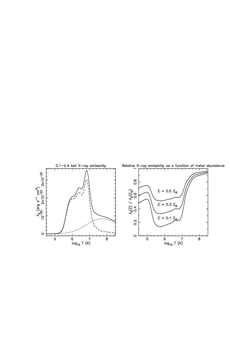
Figure 3: X-ray emissivity $\Lambda_{\rm X}$ in the $0.1$ – $2.4{\rm\thinspace keV}$ band as a function of temperature and metal abundance, assuming Solar abundance ratios and collisional ionisation equilibrium. (a) The total X-ray emissivity from the Raymond-Smith hot plasma code (Raymond & Smith 1977) for Solar metallicity (solid line), decomposed into the contribution from H and He only (dotted line) and metal ions (dashed line). (b) The soft X-ray emissivity for a hot plasma of metal abundance $Z=0.1,0.3$ and $0.5\hbox{$\thinspace{\rm Z}_{\odot}$}$, relative to the emissivity of a Solar metallicity hot plasma. For temperatures between $3\times 10^{5}{\rm\thinspace K}$ and $10^{7}{\rm\thinspace K}$ line emission from metals dominates the emission. X-ray emission from low metallicity hot plasmas is significantly depressed in this temperature range due to the lack of line emission.

The total cooling rate and X-ray emissivity of a hot gas in the temperature range $3\times 10^{5}$ – $10^{7}{\rm\thinspace K}$ is a strong function of its metal abundance, as shown in Fig. 3. Hence different explanations for the origin of the soft X-ray emission in galactic winds also imply that we expect different metal abundances for this gas and hence differing emissivities for given density and temperature. For example S94 argue that the majority of the X-ray emission from starburst driven winds is due to shocked disk material, which would have significantly lower metal abundance than the SN-enriched starburst ejecta. The metallicity of the gas in the wind will strongly affect its cooling rate and X-ray luminosity. This is unlikely to affect the dynamics of the X-ray emitting gas as it is an inefficient radiator of its thermal energy. The main effect of the assumed metallicity on the X-ray properties will be on the absolute normalisation of the X-ray luminosity, detector count rates and X-ray surface brightness from our simulations.

In the absence of more conclusive observational estimates of the metal abundance of the ISM in M82, we shall assume all the gas in these simulations is of Solar abundance. In paper II we shall investigate any biases in X-ray determined metallicities of the hot gas in galactic winds, by producing and analysing artificial X-ray observations from the multiphase gas distributions in these simulations.

2.7 Mass-loading

A starburst-driven wind, in its expansion through the ISM as a superbubble and post-blowout as a galactic wind, will overrun and envelop clumps and clouds that are denser than the ambient ISM. Once inside the bubble or wind, conductive, hydrodynamical or even photo-evaporative processes in the shocked or free wind regions will evaporate, ablate and shock-heat these clouds. This will add cool material into the hot X-ray emitting regions, and hence potentially altering the energetics and observational properties of the wind. This addition of mass into the flow is termed “mass-loading” (Hartquist et al. 1986). Unlike the interaction of the wind with the ambient, inter-cloud, medium, which adds mass to the outside of the superbubble/wind, mass-loading from clouds adds material gradually into the hot interior.

Conductive mass-loading is the evaporation of clouds by the thermal conduction of hot electrons from the hot plasma penetrating and heating the clouds (cf. Cowie et al. 1981). Hydrodynamical mass-loading is the ablation and physical destruction of clouds by hydrodynamical processes as the hot plasma flows past dense clouds, either sub-or-supersonically (Hartquist et al. 1986). Our models do not incorporate thermal conduction, so we concentrate on a hydrodynamically mass-loaded model. Although the physics of the two processes are quite different, our simple model captures the essential feature of mass-loading which is the addition of additional cold material into the hot interior of the flow. Our aim is to study the effects of a simple but physically motivated model of the interaction of the wind with dense clouds.

A dense cloud embedded in a subsonic flow will experience pressure differences along its surface that lead to it expanding perpendicularly to the direction of the surrounding flow (the head of the cloud experiences the ram pressure plus the thermal pressure of the tenuous flow, whereas the sides of the cloud only experience the thermal pressure of the surrounding flow). Rayleigh-Taylor (RT) and Kelvin-Helmholtz (KH) instabilities will remove material from the perimeter of the expanding cloud. The ablation rate of the cloud (i.e. its mass-loading rate) is proportional to the expansion speed of the cloud divided by the size of the mixing region between the cloud and the wind.

Dense clouds embedded in supersonic flows are crushed by shocks driven into them by the wind, before being disrupted by pressure differences in a similar manner to clouds in subsonic flows.

Physical arguments based on the picture given above (Hartquist et al. 1986; see Arthur & Henney 1996 for a numerical treatment of mass-loaded SNRs) suggest that the mass-loading rate $\dot{q}$ of a flow that ablates small, denser clouds depends on the Mach number $\cal M$ of the upstream flow for subsonic flows, but not for supersonic flows which are ablated at a maximum mass-loading rate $Q$, i.e.

$${\dot{q}}=\left\{\begin{array}[]{ll}Q\times{\cal M}^{4/3}&\mbox{if ${\cal M}<1.0$}\\ Q&\mbox{if ${\cal M}\geq 1.0$}.\end{array}\right.$$ (12)

In practice the maximum mass-loading rate $Q$ depends on both the properties of the cloud and the flow density and velocity. The maximum mass-loading rate per unit volume over the cloud is

$$Q=a\left(\frac{\rho_{\rm w}v_{\rm w}kT_{\rm cl}\rho_{\rm cl}^{2}}{\mu m_{\rm H}R_{\rm cl}^{3}}\right)^{1/3},$$ (13)

where $a$ is a constant of order unity, $\rho_{\rm w}$ and $v_{\rm w}$ the density and velocity of the flow the cloud is embedded in, and $T_{\rm cl}$, $\rho_{\rm cl}$, $R_{\rm cl}$ the cloud temperature, density and radius.

Despite the simplicity of this analytical treatment, numerical simulations of clouds ablated by tenuous flows (Klein, McKee & Collela 1994) support this model of mass-loading. For the purposes of these simulations we shall consider two different models of mass-loading of a starburst-driven galactic wind, based loosely on the central and distributed mass-loading model used by S96.

2.7.1 Central mass-loading

S96’s steady state mass-loaded wind models (with no ISM apart from the clouds) suggested that all mass-loading in M82 was confined to the starburst region itself. Given the observed molecular ring at a radius of $\sim 250{\rm\thinspace pc}$ from the centre, and that large masses of molecular material must have existed within the starburst region to form the young stars, it is not unreasonable to expect the majority of cloud material to exist within the starburst region.

As in S96’s model we simulate this central mass-loading by ignoring the detailed cloud mass-loading rates given above, and increasing the mass deposition rate in the starburst by a factor 5. This results in a typical mass injection rate of $\sim 5\hbox{$\thinspace{\rm M}_{\odot}$}\hbox{${\rm\thinspace yr}^{-1}\,$}$, similar to the models S96 considered most successful.

2.7.2 Distributed mass-loading

The alternative to a central reservoir of cloud material are clouds distributed throughout the disk of the galaxy. We assume all clouds have the same density, size and temperature, irrespective of their position within the galaxy. As these clouds are destroyed by the wind these properties do not alter, but only the total mass in clouds is reduced. The only cloud property we allow to vary with spatial position over the disk is the local cloud volume filling factor, which then controls the local mass in clouds. This cloud filling factor is assumed to remain constant with time, the total mass in clouds reducing with time as the wind overruns them and destroys them.

The maximum mass-loading rate $Q$ is a relatively weak function of the wind and cloud properties (as can be seen in Eqn. 13). Rather than explicitly calculate $Q$ as a function of the local flow variables at every computational cell and time step, we fix this maximum mass-loading rate over the entire grid. This allows us to explicitly control the minimum cloud destruction time-scale

$$\tau_{\rm cl}=\rho_{\rm cl}/Q,$$ (14)

where $\rho_{\rm cl}$ is the density within a cloud.

We choose $Q$ and $n_{\rm cl}$ to give a minimum cloud destruction time scale that is scientifically interesting. If the cloud destruction time-scale $\tau_{\rm cl}\ll\tau_{\rm dyn}$ (where $\tau_{\rm dyn}\sim 10{\rm\thinspace Myr}$ is the dynamical age scale of the galactic wind), then clouds will be destroyed almost instantaneously by the outer shock of the wind. All the cloud mass will be added to the outermost part of the wind, and the mass-loading will be almost identical to the evolution of a wind in a slightly denser medium. If $\tau_{\rm cl}\gg\tau_{\rm dyn}$, then almost no mass-loading will occur. Hence the case of $\tau_{\rm cl}\sim\tau_{\rm dyn}$ is the most interesting as far as the effects of mass-loading on the properties of galactic winds is concerned. We therefore set $\tau_{\rm cl}=10{\rm\thinspace Myr}$.

We assume the clouds are distributed identically to the high filling factor ambient ISM, in rotating hydrostatic equilibrium. All clouds are assumed to have number density $n_{\rm cl}=10^{3}\hbox{${\rm\thinspace cm}^{-3}\,$}$ and temperature $T_{\rm cl}=10^{3}{\rm\thinspace K}$, and apart from the assumed rotational motion, are at rest with respect to the starburst region. The total mass in clouds is almost identical in the thick and thin disk models, with a central cloud filling factor of $\eta_{\rm cl}=4\times 10^{-2}$ in the thin disk models and $\eta_{\rm cl}=1.3\times 10^{-2}$ in the thick disk models. The original mass of cloud material within the central $500{\rm\thinspace pc}$ is $\sim 3\times 10^{7}\hbox{$\thinspace{\rm M}_{\odot}$}$, and within the volume occupied by the entire galactic wind at an age $t\sim 15{\rm\thinspace Myr}$ the original cloud mass is $\sim 3\times 10^{8}\hbox{$\thinspace{\rm M}_{\odot}$}$. As the minimum cloud destruction time is $\tau_{\rm cl}=10{\rm\thinspace Myr}$, not all of this cloud mass will have been added into the flow.

At each computational step we calculate the local Mach number ${\cal M}$ and calculate the cloud mass-loading rate ${\dot{q}}$ from Eqn. 12. Note that this is the mass-loading rate per unit volume of cloud material, so the total mass-loading rate at any position is this ${\dot{q}}$ multiplied by the local cloud filling factor. We computationally track the mass remaining in clouds to ensure mass-loading ceases in regions where all the clouds have been destroyed.

Table 1: Model parameters for the twelve starburst-driven galactic wind simulations studied. The thick and thin disk ISM and gravitational potential parameters are given in Table. 2

Model	ISM	Starburst	SFH	$R_{\star}$	$H_{\star}$	Mass-loading	Grid size	Cell size
	model	mass ($\thinspace{\rm M}_{\odot}$)		(${\rm\thinspace pc}$)	(${\rm\thinspace pc}$)		(cells, r$\times$z)	(${\rm\thinspace pc}$)
tbn_1	thick	$10^{8}$	SIB	150	-	none	$400\times 800$	$14.6\times 14.6$
tbn1a	thick	$10^{8}$	SIB	150	-	none	$400\times 800$	$7.3\times 7.3$
tbn1b	thick	$10^{8}$	SIB	150	60	none	$640\times 1280$	$4.9\times 4.9$
tbn_2	thick	$10^{7}$	SIB	150	-	none	$400\times 800$	$14.6\times 14.6$
tbn_6	thick	$10^{8}$	SIB	150	-	central	$400\times 800$	$14.6\times 14.6$
tbn_7	thick	$10^{8}$	CSF	150	-	none	$400\times 800$	$14.6\times 14.6$
tbn_9	thick	$10^{8}$	SIB	150	-	distributed	$400\times 800$	$14.6\times 14.6$
mnd_3	thin	$10^{8}$	SIB	150	60	none	$480\times 800$	$14.6\times 14.6$
mnd_4	thin	$10^{7}$	SIB	150	60	none	$480\times 800$	$14.6\times 14.6$
mnd_5	thin	$10^{8}$	SIB	150	60	central	$480\times 800$	$14.6\times 14.6$
mnd_6	thin	$10^{8}$	CSF	150	60	none	$480\times 800$	$14.6\times 14.6$
mnd_8	thin	$10^{8}$	SIB	150	60	distributed	$480\times 800$	$14.6\times 14.6$

2.8 Model parameter study

We have chosen the following set of models to investigate how the dynamics and observational properties of starburst-driven galactic winds depend on the host galaxy’s ISM distribution, the starburst strength and history, and the presence and distribution of mass-loading by dense clouds. Although only comprising 12 simulations, we believe this to be the most detailed and systematic theoretical study of galactic winds to date. The model parameters for these simulations are summarised in Tables. 1 & 2.

2.8.1 Thick disk models

The thick disk models have the same ISM distributions as TB’s simulations, although run on a higher resolution computational grid. The resulting thick collimating disk allows us to investigate the effect of strong wind collimation by dense gas high above the plane of the galaxy on the wind dynamics, morphology and X-ray emission.

1. Model tbn_1 has a powerful starburst forming $10^{8}\hbox{$\thinspace{\rm M}_{\odot}$}$ of stars (assuming a Salpeter IMF between $1$ – $100\hbox{$\thinspace{\rm M}_{\odot}$}$) instantaneously within a spherical starburst region of radius $150{\rm\thinspace pc}$. To investigate the interaction of the wind with the ambient ISM alone no mass-loading is included in this simulation.

2. Model tbn1a has identical model parameters to model tbn_1, but is run on a higher resolution grid of twice the resolution to the other models (each cell is $7.3{\rm\thinspace pc}\times 7.3{\rm\thinspace pc}$), although only covering a smaller physical region. This allows us to investigate the effects of limited numerical resolution of the wind properties.

3. Model tbn1b has triple the resolution of model tbn_1, with cells $4.9{\rm\thinspace pc}\times 4.9{\rm\thinspace pc}$ in size. As with model tbn1a the aim to investigate the influence of numerical resolution. Unlike the other thick disk models the starburst region in this model is a more realistic cylindrical region also used in the thin disk models described below.

4. Model tbn_2 is almost identical to model tbn_1 with a single instantaneous starburst (SIB), except the starburst is only one tenth as powerful at that in model tbn_1. This starburst represents a lower limit on the power of the starburst in M82. In comparison with model tbn_1 this simulation allows us to investigate how wind properties and dynamics scale with starburst power.

5. Model tbn_6 has the same starburst as in model tbn_1, but mass-loading of the wind by dense clouds occurs within the starburst region (central mass-loading). This is modeled by increasing the mass injection rate from the starburst by a factor of 5.

6. Model tbn_7 has a more complex SF (CSF) history than the instantaneous starbursts used in the other models. The total mass of stars formed in the starburst is $10^{8}\hbox{$\thinspace{\rm M}_{\odot}$}$, as in model tbn_1, but the star formation is spread over a period of $10{\rm\thinspace Myr}$. This results in a more gradual deposition of mass and energy by the starburst, allowing us to investigate the effects of the history of mass and energy injection on the wind dynamics.

7. Model tbn_9 has a SIB as in model tbn_1, but also incorporates mass-loading distributed throughout the disk as discussed in Section 2.7. In combination with model tbn_6 these mass-loaded simulations allow us to investigate both the effect of mass-loading on starburst-driven winds in combination with the wind’s interaction with the ambient high filling factor ISM (unlike S96’s mass-loaded simulations, where the wind did not interact with the ambient ISM), and how the distribution of the cloud material affects the wind dynamics.

2.8.2 Thin disk models

The thin disk models include a more realistic gravitational potential than the one used in TB & S94’s simulations (and the thick disk models). This new gravitational potential approximately reproduces M82’s observed rotation curve (Fig. 1). The deeper potential results in a much thinner disk, with less collimation of the wind and lower gas density above the plane of the galaxy. We use a larger computational grid of $480\times 800$ cells covering a physical region $7.0{\rm\thinspace kpc}\times 11.6{\rm\thinspace kpc}$ to allow for the greater radial expansion of the wind in this less collimating ISM distribution.

1. Model mnd_3 differs only from model tbn_1 in its thin disk ISM distribution and more realistic gravitational potential, and its cylindrical starburst region of radius $150{\rm\thinspace pc}$ and height $60{\rm\thinspace pc}$ (i.e. extends to $z=\pm{30}{\rm\thinspace pc}$). The starburst is a SIB of total mass $10^{8}\hbox{$\thinspace{\rm M}_{\odot}$}$.

2. Model mnd_4 is a weaker SIB of mass $10^{7}\hbox{$\thinspace{\rm M}_{\odot}$}$, but otherwise is identical to model mnd_3.

3. Model mnd_5 is a centrally mass-loaded wind with otherwise identical model parameters to model mnd_3. As in the centrally mass-loaded thick disk model tbn_6 the starburst mass deposition rate has been increased by factor 5.

4. Model mnd_6 explores the same complex SF history as model tbn_7 but in a thin disk ISM.

5. Model mnd_7 is a thin disk model with a SIB of mass $10^{8}\hbox{$\thinspace{\rm M}_{\odot}$}$ that incorporates distributed mass-loading. The total mass in clouds is very similar to model tbn_9, although the clouds are distributed within a thin disk.

Table 2: Thick and thin disk ISM parameters

Parameter	Thick disk models	Thin disk models
$M_{\rm ss}$ ($\thinspace{\rm M}_{\odot}$)	$1.2\times 10^{9}$	$2\times 10^{8}$
$\omega_{0}$ (${\rm\thinspace pc}$)	350	350
$M_{\rm disk}$ ($\thinspace{\rm M}_{\odot}$)	-	$2\times 10^{9}$
$a$ (${\rm\thinspace pc}$)	-	222
$b$ (${\rm\thinspace pc}$)	-	75
$n_{\rm disk,0}$ (${\rm\thinspace cm}^{-3}\,$)	$20$	$20$
$c_{\rm s,disk}$ (${\rm\thinspace km}{\rm\thinspace s}^{-1}\,$)	$30$	$30$
$T_{\rm disk,0}$ (${\rm\thinspace K}$)	$6.5\times 10^{4}$	$6.5\times 10^{4}$
$n_{\rm halo,0}$ (${\rm\thinspace cm}^{-3}\,$)	$2\times 10^{-3}$	$2\times 10^{-3}$
$c_{\rm s,halo}$ (${\rm\thinspace km}{\rm\thinspace s}^{-1}\,$)	$300$	$300$
$T_{\rm halo,0}$ (${\rm\thinspace K}$)	$6.5\times 10^{6}$	$6.5\times 10^{6}$
$e_{\rm rot}$	0.90	0.95
$Z$ ($\thinspace{\rm Z}_{\odot}$)	1.0	1.0

3 Results

Table 3: Galactic wind properties in all the models at $t=7.5{\rm\thinspace Myr}$. Note that these values account for both lobes of the bipolar wind, except the quoted sizes, which are measured from the centre of the galaxy. The input parameters for the different models can be found in Tables 1 and 2.

Property	Units	tbn_1	tbn1a	tbn1b	tbn_2	tbn_6	tbn_7	tbn_9	mnd_3	mnd_4	mnd_5	mnd_6	mnd_7
$L_{\rm W}^{a}$	$10^{40}\hbox{${\rm\thinspace erg}{\rm\thinspace s}^{-1}\,$}$	206.0	206.0	206.0	20.6	206.0	210.0	206.0	206.0	20.6	206.0	210.0	206.0
$L_{\rm X,soft}^{b}$	$10^{40}\hbox{${\rm\thinspace erg}{\rm\thinspace s}^{-1}\,$}$	18.78	12.08	6.92	0.84	57.49	14.45	36.86	0.63	0.07	22.38	0.88	3.67
$L_{\rm X,hard}^{c}$	$10^{38}\hbox{${\rm\thinspace erg}{\rm\thinspace s}^{-1}\,$}$	8.22	8.12	6.14	0.19	51.76	3.89	13.96	5.92	1.77	40.18	2.11	7.09
$F_{\rm X,int}^{d}$	count  s${}^{-1}\,$	30.68	19.05	10.76	1.37	79.1	24.00	50.12	0.83	0.08	21.36	1.27	5.61
$F_{\rm X,abs}^{e}$	count  s${}^{-1}\,$	1.65	1.40	1.00	0.05	11.85	1.02	7.16	0.13	0.02	9.29	0.07	0.74
$E_{\rm inj}^{f}$	$10^{56}{\rm\thinspace erg}$	7.10	7.10	7.10	0.71	7.10	2.53	7.10	7.10	0.71	7.10	2.53	7.10
$E_{\rm th}^{g}$	$10^{56}{\rm\thinspace erg}$	1.55	1.35	1.15	0.15	0.75	0.65	1.53	2.47	0.44	0.81	1.15	2.57
$E_{\rm th,z>1.5}^{g}$	$10^{56}{\rm\thinspace erg}$	1.06	0.73	0.80	0.02	0.17	0.27	0.53	2.31	0.40	0.61	1.03	2.28
$E_{\rm KE}^{h}$	$10^{56}{\rm\thinspace erg}$	2.73	2.51	3.21	0.19	3.13	1.08	2.74	4.86	0.35	5.75	1.78	4.70
$E_{\rm KE,z>1.5}^{h}$	$10^{56}{\rm\thinspace erg}$	2.04	1.71	2.58	0.04	1.51	0.51	1.63	4.27	0.30	4.28	1.22	4.05
$M_{\rm inj}^{f}$	$10^{7}\hbox{$\thinspace{\rm M}_{\odot}$}$	1.20	1.20	1.20	0.12	1.20	0.43	1.20	1.20	0.12	1.20	0.43	1.20
$M_{\rm gas}^{i}$	$10^{7}\hbox{$\thinspace{\rm M}_{\odot}$}$	56.5	54.8	49.4	19.5	56.8	30.9	61.1	18.9	8.0	21.1	11.7	24.9
$M_{\rm gas,z>1.5}^{i}$	$10^{7}\hbox{$\thinspace{\rm M}_{\odot}$}$	9.6	6.7	7.4	0.4	6.1	2.5	7.5	4.0	0.9	5.8	2.0	5.4
$\eta_{\rm warm}^{j}$	-	0.10	0.12	0.11	0.20	0.38	0.13	0.17	0.21	0.12	0.23	0.20	0.08
$f_{\rm M,warm}^{k}$	-	0.06	0.04	0.04	0.013	0.05	0.03	0.04	0.04	0.03	0.13	0.05	0.12
$f_{\rm TH,warm}^{l}$	-	0.11	0.10	0.11	0.06	0.17	0.07	0.09	0.02	0.04	0.17	0.03	0.07
$f_{\rm KE,warm}^{m}$	-	0.21	0.22	0.19	0.11	0.31	0.15	0.14	0.33	0.16	0.30	0.27	0.05
$\log n_{\rm e,warm}^{n}$	${\rm\thinspace cm}^{-3}\,$	-0.77	-0.80	-0.98	-1.06	-0.52	-0.62	-0.63	-2.15	-2.30	-1.54	-1.80	-1.52
$v_{\rm warm}^{o}$	${\rm\thinspace km}{\rm\thinspace s}^{-1}\,$	621	668	802	433	745	646	607	1936	1143	732	1579	289
$\eta_{\rm hot}^{p}$	-	0.81	0.75	0.83	0.55	0.32	0.72	0.77	0.71	0.82	0.55	0.80	0.87
$f_{\rm M,hot}^{q}$	-	0.03	0.03	0.04	0.005	0.03	0.02	0.07	0.18	0.11	0.08	0.15	0.18
$f_{\rm TH,hot}^{r}$	-	0.57	0.45	0.66	0.23	0.61	0.40	0.78	0.83	0.88	0.76	0.89	0.81
$f_{\rm KE,hot}^{s}$	-	0.49	0.41	0.59	0.16	0.15	0.46	0.50	0.56	0.74	0.53	0.66	0.89
$\log n_{\rm e,hot}^{t}$	${\rm\thinspace cm}^{-3}\,$	-2.04	-1.91	-2.02	-2.15	-0.79	-1.82	-1.31	-2.65	-2.76	-1.50	-2.74	-2.40
$v_{\rm hot}^{u}$	${\rm\thinspace km}{\rm\thinspace s}^{-1}\,$	804	742	836	660	591	889	735	772	644	331	693	815
$z_{\rm max}^{v}$	${\rm\thinspace pc}$	7088	5826	6217	3471	4025	5469	6329	8444	5338	6635	6796	7831
$r_{\rm max}^{w}$	${\rm\thinspace pc}$	2888	2392	2460	1327	1546	1983	2115	5513	3675	4404	4696	5119
$r_{\rm base}^{x}$	${\rm\thinspace pc}$	1167	1096	1102	695	1259	841	1220	1220	763	1395	904	1045

^a Starburst mechanical energy injection rate averaged over the period between $t=6.5$ and $7.5{\rm\thinspace Myr}$.

^b Intrinsic soft X-ray luminosity in the ROSAT $0.1$ – $2.4{\rm\thinspace keV}$ band.

^c Intrinsic hard X-ray luminosity in the $2.4$ – $15.0{\rm\thinspace keV}$ energy band.

^d ROSAT PSPC count rate assuming no absorption and distance $D=3.63{\rm\thinspace Mpc}$ to M82.

^e ROSAT PSPC count rate assuming a uniform hydrogen column of $\hbox{$N_{\rm H}$}=4\times 10^{20}\hbox{${\rm\thinspace cm}^{-2}\,$}$ (the Galactic column density towards M82, Stark et al. 1992) and distance $D=3.63{\rm\thinspace Mpc}$ to M82.

^f Total energy and mass injected from SNe and stellar winds in the starburst up to this time.

^g Total thermal energy within the entire wind ($E_{\rm TH}$), and within those parts of the wind lying above $z=1.5{\rm\thinspace kpc}$ ($E_{\rm TH,z>1.5}$).

^h Total kinetic energy within the entire wind ($E_{\rm KE}$), and within those parts of the wind lying above $z=1.5{\rm\thinspace kpc}$ ($E_{\rm KE,z>1.5}$).

ⁱ Total gas mass within the entire wind and within the wind lying above $z=1.5{\rm\thinspace kpc}$

^j Volume filling factor of the warm ($5.5\leq\log T({\rm\thinspace K})<6.5$) gas.

^k to ^m Fraction of total gas mass ($f_{\rm M}$), thermal energy ($f_{\rm TH}$) and kinetic energy ($f_{\rm KE}$) in warm gas.

ⁿ Root mean square electron density of warm gas within the wind.

^o Volume-averaged velocity of warm gas.

^p to ^u As $i$ – $o$ but for hot ($6.5\leq\log T({\rm\thinspace K})<7.5$) gas.

^v Maximum extent of the wind (the position of the outermost shock) along the minor axis measured from the nucleus of the galaxy.

^w Maximum radial extent of the wind, measured from the minor axis.

^x Maximum radial extent of the wind in the plane of the galaxy (i.e. at $z=0$).

We shall concentrate on three main topics in this present paper: (a) wind growth and outflow geometry, in particular the issues of wind collimation and confinement; (b) the origin and physical properties of the soft X-ray emitting gas in these winds, in particular the filling factor of the X-ray dominant gas, and (c) the previously unexplored aspects of wind energetics and energy transport efficiencies.

The observable X-ray properties of these models, i.e. simulated X-ray imaging and spectroscopy, will be in the second paper of this series. Also deferred to Paper II is the discussion of which model parameters seem best to describe M82’s observed properties.

Table 3 provides a general compilation of physically interesting wind properties in all twelve of the models at a fairly typical epoch of wind growth, $7.5{\rm\thinspace Myr}$ after the start of the starburst.

For descriptive convenience we shall define gas temperatures in the following terms. In general, “cool” gas has temperatures in the range $4.5\leq\log T({\rm\thinspace K})<5.5$, “warm” gas lies in the range $5.5\leq\log T({\rm\thinspace K})<6.5$, “hot” gas has $6.5\leq\log T({\rm\thinspace K})<7.5$ and “very hot” gas has temperatures $7.5\leq\log T({\rm\thinspace K})<8.5$.

3.1 Wind growth and outflow geometry

In this section we shall concentrate on the intrinsic morphology of the wind, in particular opening angles and the radius of the wind in the plane of the galaxy, as well as the qualitative wind structure in comparison to standard wind-blown bubbles. We shall consider the information X-ray surface brightness morphology provides separately in Paper II.

Morphological information on the wind geometry in M82 is primarily based upon optical and X-ray observations. Optical emission line studies such as Heckman et al. (1990), Götz et al. (1990) & McKeith et al. (1995) constrain the cool-gas outflow geometry strongly within $z\mathrel{\hbox to0.0pt{\lower 3.0pt\hbox{$\sim$}\hss}\raise 2.0pt\hbox{$<$}}2{\rm\thinspace kpc}$ of the plane of the galaxy, using spectroscopy and imaging. Narrow-band optical imaging can trace the wind out to $z\sim 6{\rm\thinspace kpc}$. X-ray observations by the ROSAT PSPC and HRI also trace the warm and hot phases of the wind out to $z\sim 6{\rm\thinspace kpc}$ from the plane, but suffer from poor resolution and point source confusion near the plane of the galaxy.

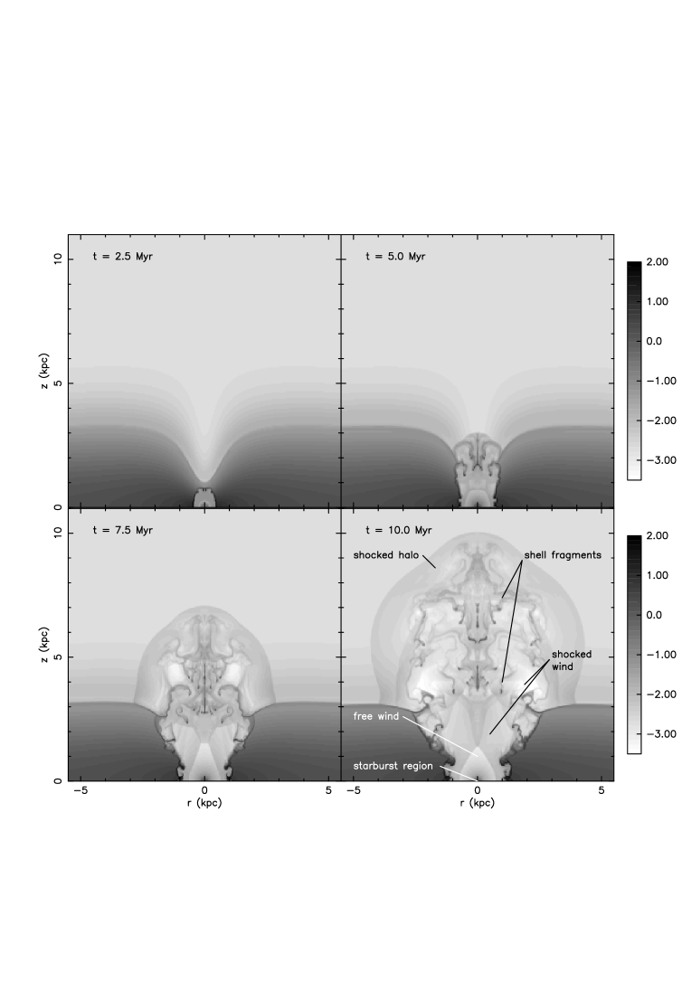
Figure 4: The logarithm of the wind number density in the thick disk model tbn_1 at four epochs. The intensity scale extends between $-3.5\leq\log n(\hbox{${\rm\thinspace cm}^{-3}\,$})\leq 2.0$, and number densities above or below this range are shown as black or white respectively. The final panel labels some important features of the wind: the starburst region in the nucleus of the galaxy, the freely expanding wind, shocked wind, shocked disk and halo gas, and superbubble shell fragments. Note that these numerical simulations assume cylindrical symmetry around the $z$-axis, so the shell fragments are actually annuli. Note the very small region of freely expanding wind, the initially cylindrical geometry of the wind opening out with time into a truncated cone, and the increasing size of the wind in the plane of the galaxy.

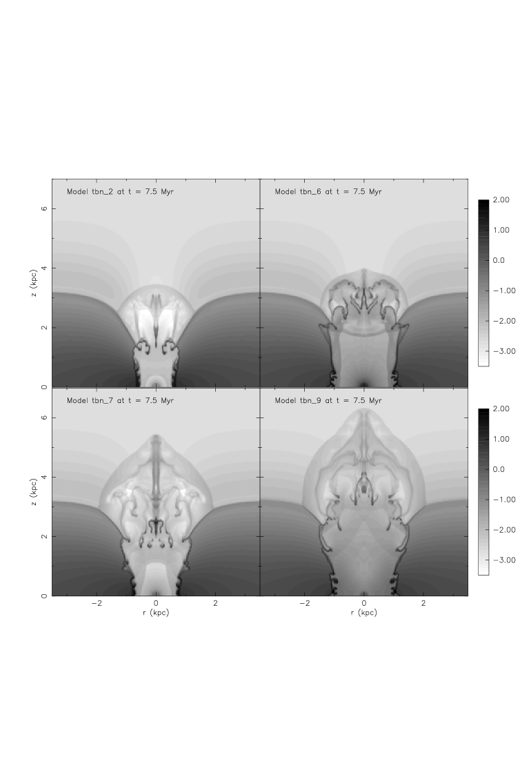
Figure 5: The logarithm of the wind number density in the thick disk models tbn_2, tbn_6, tbn_7 & tbn_9 at $t=7.5{\rm\thinspace Myr}$. The intensity scale extends between $-3.5\leq\log n(\hbox{${\rm\thinspace cm}^{-3}\,$})\leq 2.0$, and number densities above or below this range are shown as black or white respectively. The weaker starburst tbn_2 (a factor 10 less powerful than model tbn_1) leads to a smaller but otherwise structurally similar wind to model tbn_1. In model tbn_6 the cooler and denser wind (due to the additional mass injection within the starburst region) significantly alters the structure of the regions of shocked wind material within the galactic wind, and reduces its expansion rate. The more gradual energy injection rate of model tbn_7 compared to model tbn_1 also reduces the wind’s growth rate, but otherwise this model is very similar to model tbn_1. The interior structure of the wind in model tbn_9 is much more homogeneous than the other thick disk models due the enhanced wind density due to distributed mass-loading, and it is difficult to distinguish separate free wind and shocked wind regions.

3.1.1 Wind density structure

As an effective visual method of illustrating galactic wind evolution and growth, and some of the differences between the various models, we reproduce grey-scale images of $\log$ number density in the $r$-$z$ plane in Figs. 4 – 7. These show the wind at $2.5{\rm\thinspace Myr}$ intervals up to $t=10{\rm\thinspace Myr}$ in models tbn_1 and mnd_3, and at $t=7.5{\rm\thinspace Myr}$ in all the other models excepting models tbn1a & tbn1b.

We shall briefly describe the evolution and structure of the wind in model tbn_1 (see Fig. 4), a single instantaneous starburst occurring in the thick disk ISM, and then discuss the differences in the evolution of the wind in the other models to this model. Differences between model tbn_1 and the higher resolution models tbn1a and tbn1b are discussed in Section 4 along with a general discussion of the effects of finite numerical resolution.

At $t=2.5{\rm\thinspace Myr}$ the starburst-driven superbubble has yet to blow out of the thick disk, although it is elongated along the minor axis. Although difficult to see when shown to scale alongside the later stages of the wind, the superbubble has a standard structure of starburst region, free wind, shocked wind and a denser cooler shell of swept-up and shocked disk material.

By $t=5{\rm\thinspace Myr}$ the superbubble has blown out, the dense superbubble shell fragmenting under Rayleigh-Taylor (RT) instabilities. The superbubble shell was RT-stable as long as it was decelerating, but the negative density gradient along the $z$-axis and the sudden influx of SN energy at $t\sim 3{\rm\thinspace Myr}$ rapidly accelerate the shell along the minor axis after $t\sim 3{\rm\thinspace Myr}$. The internal structure of the wind is more complex than the superbubble described above. A new shell of shocked halo matter forms, but given its low density and high temperature it never cools to form a dense shell as in the superbubble phase. The re-expanding shocked wind can be seen to be ablating the shell fragments. Note also the structure of the reverse shock terminating the free wind region, which is no longer spherical. The oblique nature of this shock away from the minor axis acts to focus material out of the plane of the galaxy, as first described by TI. The combination of the disk density gradient and this shock-focusing make the wind cylindrical at this stage.

Note that the complex structure of the wind after blowout and shell fragmentation means that it is not meaningful to model the emission from interior of a galactic wind using the standard Weaver et al. (1977) similarity solutions. Nevertheless, semi-analytical models based on the thin-shell approximation (e.g. Mac Low & McCray 1988; Silich & Tenorio-Tagle 1998) can be used to explore the location of the outer shock of the wind with good accuracy, provided the radiative losses from the interior of the wind are not significant. Tracking the location of the outer shock is perhaps only important in assessing if a superbubble of a set mechanical energy injection rate can blow out of a given ISM distribution. Calculations of observable properties and the long term fate of the matter in any outflow do require the use of multidimensional hydrodynamical simulations.

The wind geometry within the disk is similar to a truncated cone at $t=7.5{\rm\thinspace Myr}$. In the halo the outer shock propagating in the halo becomes more spherical as the anisotropy of the ISM reduces with increasing distance along the $z$-axis. The structure of the shocked wind region is becoming even more complex, as it interacts with the superbubble shell fragments. The shell fragments are steadily being carried out of the disk, although being slowly spread out over a larger range of $z$ with time. The shocked wind also interacts with the disk, removing disk gas and carrying it slowly out of the disk.

At $t=10{\rm\thinspace Myr}$ the wind has increased in size, but remains qualitatively very similar in structure to the wind at $t=7.5{\rm\thinspace Myr}$. Shell fragments are spread between $3.5\leq z\leq 7{\rm\thinspace kpc}$, a large range given their common origin in the superbubble shell. Long tails can be seen extending from the shell fragments, their curling shapes tracing the complex flow pattern within the shocked wind. Regions of expansion followed by new internal shocks can also be seen within the shocked wind, a marked difference from the structure of conventional wind blown bubbles.

With mass and energy injection rates from the starburst reduced by a factor 10 from model tbn_1, the wind in model tbn_2 evolves at a slower pace than model tbn_1 (see Fig. 5). The eventual wind structure is very similar to that of model tbn_1, although disruption of the disk appears reduced and the wind remains more cylindrical within the disk. From standard self-similar wind blown bubble theory (Weaver et al. 1977) the size of a pressure-driven bubble is only a weak function of the energy injection rate, $R\propto L_{\rm w}^{1/5}$, so we might expect model tbn_2 to be $\sim 60$% the size of model tbn_1 at any given epoch. In practice model tbn_2 is less than 60% the size of model tbn_1 at the same epoch, which may be due the increased relative importance of radiative cooling in depressurising tbn_2’s wind, given that the cooling time-scales are the same in both simulations.

The wind in model tbn_6 (Fig. 5) grows at slower rate than model tbn_1 despite having exactly the same energy injection history. In this case the reduced growth must be due to the central mass-loading used. The mass injection rate within the starburst has been increased by a factor 5 from that due to stellar winds and SNe alone, representing the entrainment of dense gas remaining from the star formation. The central mass-loading increases the density of the free wind by a factor $5^{3/2}\approx 11$, due to the additional mass and the reduced outflow rate (as the energy per particle is less), and reduces the temperature of the gas by a factor $5$ from $\sim 1.5\times 10^{8}{\rm\thinspace K}$ to $\sim 3\times 10^{7}{\rm\thinspace K}$. Despite the enhanced density of the material ejected from the starburst, the wind retains recognisable features of shell fragments and shocked halo, although their dynamics and morphology have clearly been altered by the denser, slower wind fluid in this model.

Model tbn_7 (Fig. 5) was chosen to investigate the effect of a more gradual energy and mass injection history than the instantaneous starburst used in the other models (see Fig. 2). Apart from the resulting slightly slower growth, the structure of the wind in this model is very similar to that in model tbn_1.

The distributed mass-loading in model tbn_9 significantly increases the density of what would be the free and/or shocked wind regions. Note the apparent lack of an obvious shock separating the free wind and shocked wind regions in this model (Fig. 5). This is not unexpected, as distributed mass-loading has the interesting property of increasing the Mach number of subsonic flows while reducing the Mach number in supersonic flows, to produce a flow with a Mach number of order unity (Hartquist et al. 1986). As in model tbn_6 the wind’s growth is slightly slower than the non-mass-loaded model tbn_1.

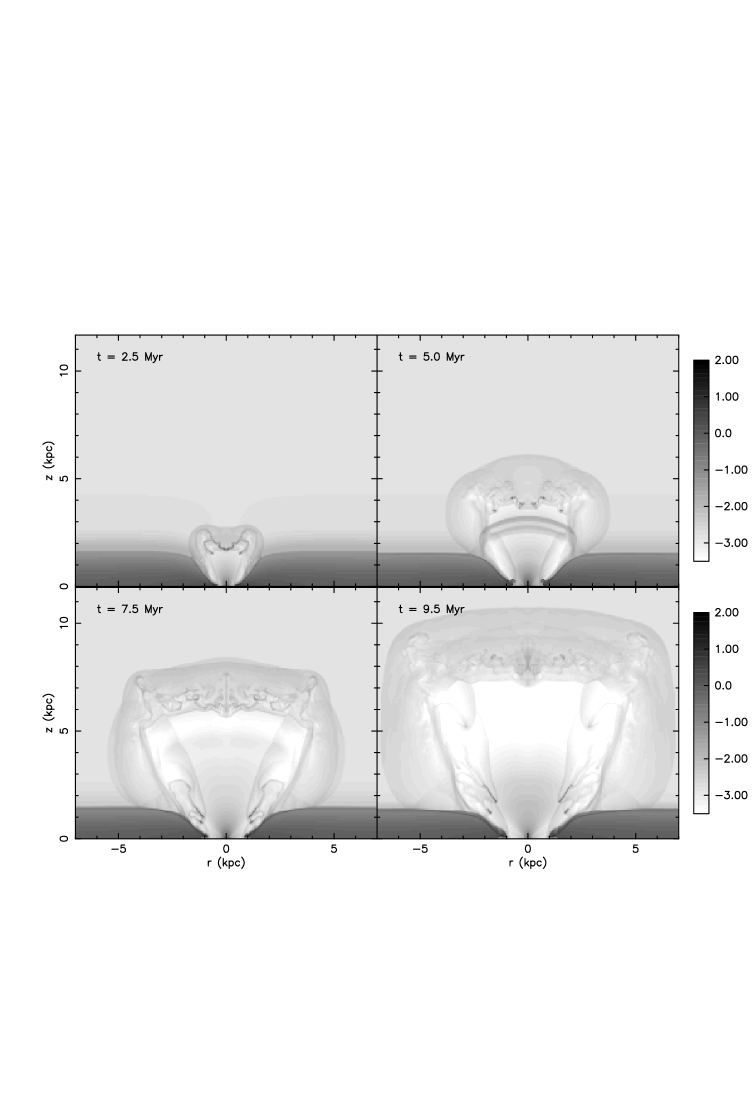
Figure 6: The logarithm of the wind number density in the thin disk model mnd_3 at four epochs. The intensity scale extends between $-3.5\leq\log n(\hbox{${\rm\thinspace cm}^{-3}\,$})\leq 2$, and number densities above or below this range are shown as black or white respectively. In comparison with the thick disk model tbn_1 note the very large volume occupied by the freely expanding wind and the large opening angle. Due to the lack of disk material above the starburst the importance of shocked disk and shell fragments is reduced in these thin disk models.

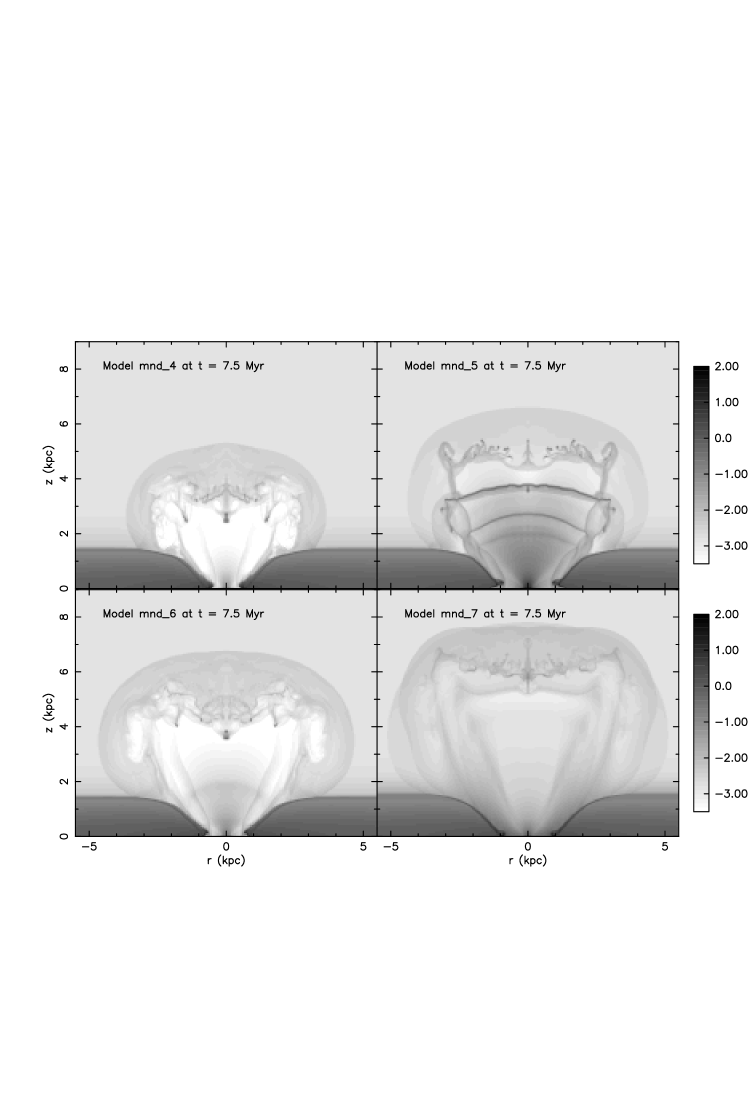
Figure 7: The logarithm of the wind number density in the thin disk models mnd_4, mnd_5, mnd_6 & mnd_7 at $t=7.5{\rm\thinspace Myr}$. The intensity scale extends between $-3.5\leq\log n(\hbox{${\rm\thinspace cm}^{-3}\,$})\leq 2$, and number densities above or below this range are shown as black or white respectively. The weak starburst in model mnd_4 leads to a smaller free wind region, and the majority of the outflow volume is occupied by shocked halo material. In model mnd_5, as in model tbn_6, the cooler and denser mass-loaded wind alters the structure of the regions of shocked wind material within the galactic wind. The sharp features seen propagating out in the free wind are due to periods of increased mass injection in the instantaneous starburst model used (see Fig. 2). The simple model for central mass-loading used assumes the total mass-loading rate in the starburst region is just a multiple of the starburst mass injection rate. A more realistic model of starburst history and mass-loading would lead to a smoother mass injection rate. The more gradual energy injection rate of model mnd_6 compared to the instantaneous burst model mnd_3 reduces the wind’s growth rate slightly, but otherwise this model is very similar to model mnd_3. In model mnd_7 the density of the free wind is increased due to distributed mass-loading. As the clouds are assumed to be distributed in the same way as the ambient ISM the majority of the mass-loading occurs not near the $z$-axis but near the outer edge of the wind.

The wind structure in model mnd_3 (Fig. 6) is significantly different from model tbn_1 due to the thin, less-collimating disk used in this and the following models. The lack of substantial amounts of dense gas above the starburst region allows very rapid blowout of the wind, easily shattering a much less massive superbubble shell. The net result is a wind with a larger opening angle (due to the lack of any significant collimation by the disk), a very large free wind region, and an indistinct region of shocked wind and shocked disk material surrounded by the standard shocked halo region. The few superbubble fragments rather rapidly loose definition and are mixed in with the shocked wind by $t\sim 7.5{\rm\thinspace Myr}$. Due to the early blowout into the halo and lack of collimation the wind is much more spherical than the thick disk models.

The morphology of the weak starburst model mnd_4 (Fig. 7) is generally similar to that of model mnd_3, although with two interesting exceptions. The much less energetic wind is not able to punch out into the halo as effectively as the wind in model mnd_3. A weak, almost spherical, shock wave does propagate out into the halo, leading to a wind with much of the volume being shocked halo material. Also note the free wind is confined to a narrow region along the $z$-axis by shocked wind material flowing up out of the disk. This flow of shocked wind is also present in the other thin disk models, and is responsible for their peculiar, almost box like, morphology.

The structure and growth of the central mass-loaded thin disk model mnd_5, the complex star formation history model mnd_6, the distributed mass-loading model mnd_7 (see Fig. 7) are related to the basic thin disk model mnd_3 in the same way as the equivalent thick disk models are related to model tbn_1.

The main differences between the thin disk models and the thick disk models are the lack of collimation in the thin models, the resulting large regions of freely expanding wind, and less complex shocked wind and disk regions with shell fragments that are disrupted and mixed into the flow at an earlier stage.

3.1.2 Wind growth

The vertical and radial growth of the galactic winds as a function of time in these models is shown in Fig. 8. The maximum vertical extent of the wind (almost invariably size of wind on the $z$-axis) $z_{\rm max}$, maximum radial extent $r_{\rm max}$ and radius of the base of the wind $r_{\rm base}$ in all the models can be seen to be well behaved power laws (or broken power laws) in time.

The vertical and radial growth rates in the thick disk models clearly differ from those in the thin disk models. The thick disk models all show initially slow vertical ($z_{\rm max}$) and radial growth ($r_{\rm max}$), followed by rapid acceleration. The wind begins to accelerate along the $z$-axis after $t\sim 3{\rm\thinspace Myr}$, and later along the $r$-axis, $t\sim 5{\rm\thinspace Myr}$. The initial evolution is similar to that predicted by the Weaver et al. (1977) model of a pressure driven bubble in a constant density medium, i.e. $R\propto t^{0.6}$. The later phase of acceleration is caused by both the superbubble “running down” the ISM density gradient leading into the halo, and the dramatic increase in mechanical energy injection rate at $t\sim 3{\rm\thinspace Myr}$ due to the first SNe. At later times the wind should return to the $R\propto t^{0.6}$ expansion law once in the almost constant density halo. The initial stages of this final deceleration may be what is seen in Fig. 8 at late times in models tbn_2 and tbn_7.

In contrast the wind in the thin disk models shows no evidence for periods of increased or decreased acceleration over the simulation. Measured over the period from $t=0.5{\rm\thinspace Myr}$ until the end of the simulation the wind is constantly accelerating both vertically ($1.10\leq\partial\log z_{\rm max}/\partial\log t\leq 1.37$) and radially ($1.04\leq\partial\log r_{\rm max}/\partial\log t\leq 1.25$) in all the thin disk models. The thin disk allows the wind to blow out very early in its evolution, and it gradually runs down the density gradient into the halo.

In all the models (both thin and thick disk) the growth of the wind in the plane of the galaxy ($r_{\rm base}$) is well approximated by the expansion law of a constant power bubble expanding into a uniform medium. The base of the wind expands at a rate $\partial\log r_{\rm base}/\partial\log t\sim 0.6$, measured over the period $t=0.5{\rm\thinspace Myr}$ until the end of the simulation. The range in slope around the expected value of 0.6 is small, from 0.53 (model mnd_6) to 0.67 (model tbn_9), and does not deviate in any clear systematic manner due to mass-loading, the ISM distribution or the star formation history.

There is no evidence for a change in $\partial\log r_{\rm base}/\partial\log t$ once the wind has broken out, as might be expected if blowout leads to a depressurisation of the wind. The evolution of the hot gas in the plane of the galaxy does not appear to be affected by the blowout over the period covered by our simulations.

Figure 8: Vertical and radial growth of all the wind models as a function of time. The initial evolution of the maximum vertical size $z_{\rm max}$, maximum radial size $r_{\rm max}$ and size of the wind in the plane of the galaxy $r_{\rm base}$ for the thick disk models, obeys the $R\propto t^{0.6}$ law expected of confined pressure-driven bubbles. Post blow out (which occurs almost instantaneously in the thin disk models) $z_{\rm max}$ and $r_{\rm max}$ grow more rapidly, as the wind accelerates down the density gradient into the halo.

3.1.3 Wind collimation and opening angles

The density distributions shown in Figs. 4 – 7 clearly demonstrate that the main factor controlling the wind morphology is the disk ISM distribution. The thick disk ISM models produce initially cylindrical winds that evolve into collimated truncated conical winds with low opening angles. The thin disk models invariably produce conical winds with large opening angles.

These outflow geometries should be compared to that inferred from optical observations of M82 (see Fig. 9), of an initially conical wind ($r\sim 420{\rm\thinspace pc}$ for $z\leq 330{\rm\thinspace pc}$) flaring out above $z=330{\rm\thinspace pc}$ into a cone of opening angle $\theta\sim 30\hbox{${}^{\circ}$}$ (based on Götz et al. 1990; McKeith et al. 1995, scaled to our assumed distance of $3.63{\rm\thinspace Mpc}$ to M82).

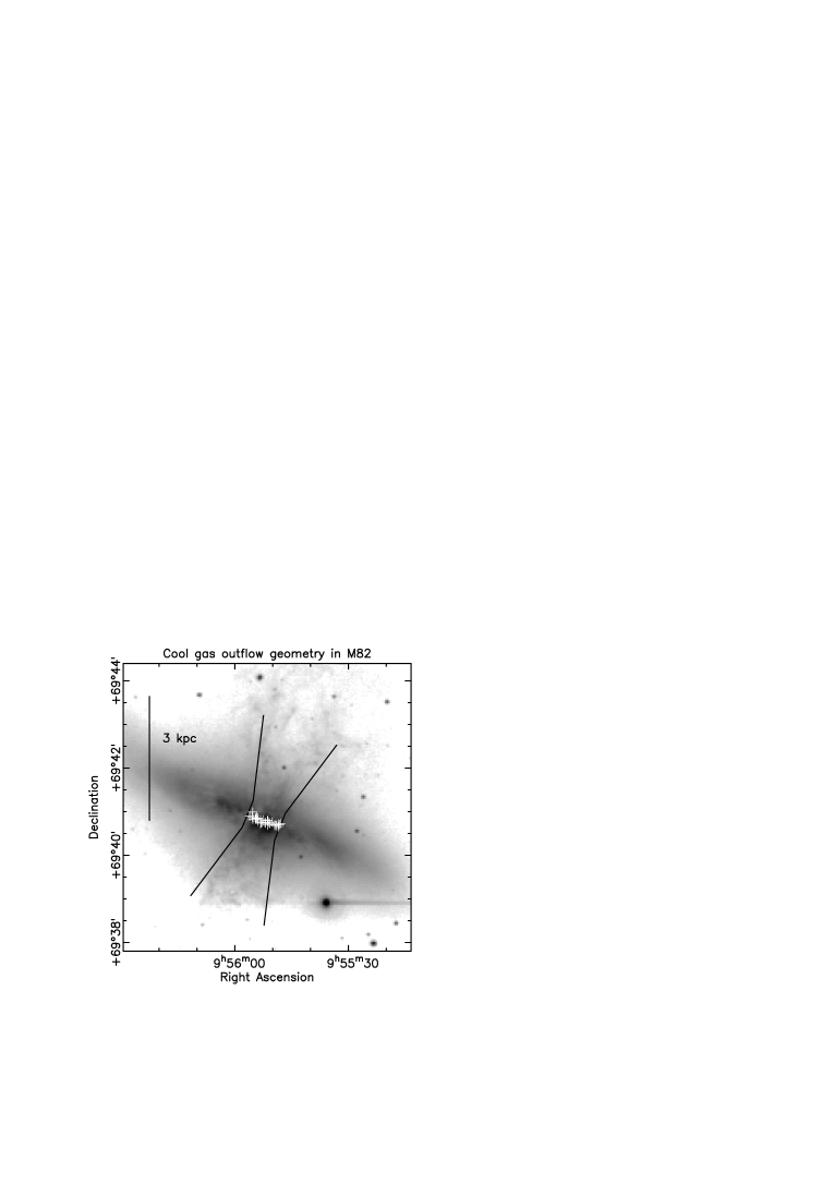
Figure 9: The wind outflow geometry in M82 based on the work of Götz et al. (1991) and McKeith et al. (1995), overlaid on a ${\rm H}\alpha$ image. The young supernova remnants (Muxlow et al. 1994) marking the starburst region are shown as a series of white crosses.

Measuring the wind opening angles in our models as a function of time, it is clear that the thin disk models fail to produce such a well collimated wind. The opening angle is $\theta_{\rm thin}\sim 90\hbox{${}^{\circ}$}$ in model mnd_3 at all epochs, which is typical of all the thin disk models.

In comparison the thick disk models (deliberately chosen to provide a collimating ISM distribution) are much more successful, although even in these models the opening angles can become too large to be a good match for M82 at late times. The opening angles in the thick disk models do show some variation between the different models, but typically the wind is initially spherical in its superbubble phase, becoming much more cylindrical (i.e. $\theta\sim 0\hbox{${}^{\circ}$}$) as it begins to blow out. Post-blowout the opening angles are typically $\theta_{\rm thick}\sim 40\hbox{${}^{\circ}$}$, but this masks a general increase from $\theta\sim 0\hbox{${}^{\circ}$}$ at $t\sim 5{\rm\thinspace Myr}$ to $\theta\sim 60\hbox{${}^{\circ}$}$ at $t\sim 10$ – $15{\rm\thinspace Myr}$. More gentle energy injection histories, as in models tbn_2 and tbn_7, do give slightly lower opening angles at a given epoch than in model tbn_1, confirming S94’s conclusion that weak initial winds can reduce later disruption of the disk by the more energetic phases of the starburst. Note that this is a weak effect in the simulations we consider, and the main factor affecting wind geometry is the initial ISM distribution, not the starburst energy injection history.

It is clear that a thick, collimating ISM distribution seems necessary to reproduce the observed narrow, low opening angle, wind in M82. Even our thick disk model does not provide sufficient collimation.

3.1.4 Confinement

TT’s criticism that the size of the base of the wind is too large in TB and S94’s simulations remains true in these simulations. The radius of the wind in the plane of the galaxy grows larger than that observed in M82, and shows no signs of slowing down as can be seen Fig. 8.

Götz et al. ’s (1990) observations limit the radius of the wind to $r\sim 420{\rm\thinspace pc}$ at $z\sim 110{\rm\thinspace pc}$ above the plane of the galaxy. This radius is very similar to the extent of the SN remnants that measure the current SN rate (see Fig. 9).

In contrast $r_{\rm base}\sim 1500{\rm\thinspace pc}$ in model mnd_3 at $t=9.5{\rm\thinspace Myr}$, a factor ten larger than the assumed starburst region. All the simulations have base radii in the range $r_{\rm base}\sim 1$ – $2{\rm\thinspace kpc}$ at $t\sim 10{\rm\thinspace Myr}$. A dramatic reduction in starburst power by a factor ten (model tbn_1 to model tbn_2) only reduces $r_{\rm base}$ from $\sim 1400{\rm\thinspace pc}$ to $\sim 850{\rm\thinspace pc}$ at $t=10{\rm\thinspace Myr}$.

By $t=5{\rm\thinspace Myr}$ the base of the wind is too large in all the models, so to explain this problem away with the ISM distributions we have used would require M82’s starburst to be very young, i.e. $t<5{\rm\thinspace Myr}$. This is difficult to justify observationally, and as we shall show in Paper II, the observed X-ray extent of the wind requires a slightly older wind ($t\mathrel{\hbox to0.0pt{\lower 3.0pt\hbox{$\sim$}\hss}\raise 2.0pt\hbox{$>$}}7.5{\rm\thinspace Myr}$).

TT constructed steady state models of bipolar outflows from starburst galaxies, where the ram pressure of infalling dense molecular gas confines the radius of the base of the wind to a fixed position. Although this solves the confinement problem, their model requires unphysically large masses of gas to be falling in along the plane of the galaxy. For example, in the model published in Tenorio-Tagle & Muñoz-Tuñón (1998), the mass of the ISM within central kiloparsec is $M_{\rm gas}\sim 5\times 10^{9}\hbox{$\thinspace{\rm M}_{\odot}$}$, where observations of M82 limit the total mass of the ISM to be $\mathrel{\hbox to0.0pt{\lower 3.0pt\hbox{$\sim$}\hss}\raise 2.0pt\hbox{$<$}}10^{8}\hbox{$\thinspace{\rm M}_{\odot}$}$ within the same radius.

Dense molecular gas, even if not falling into the nuclear region, may nonetheless be important for confining the base of the wind. CO observations (Nakai et al. 1987) reveal a molecular “ring” extending in radius between $r\sim 100$ – $400{\rm\thinspace pc}$, at the outer edge of which spurs of molecular material emerge perpendicular to the plane and extend $\sim 500{\rm\thinspace pc}$ from the disk. Much of the gas mass within the central kiloparsec is probably within this molecular gas. It may be that this molecular ring can provide the wind with enough resistance to slow its expansion in the plane of the galaxy. Although this molecular gas does not have a volume filling factor of order unity as envisioned by TT (see Lugten et al. [1986]), its areal filling factor may be high, and it undoubtedly could strongly mass-load the wind in the plane of the galaxy. Further simulations explicitly including a molecular ring are currently in progress to explore this possibility.

Somewhat more speculatively, magnetic fields might collimate the wind (e.g. de Gouveia Dal Pino & Medina Tanco 1999). We do not believe pursuing this option is currently necessary, given that the alternatives have not yet been explored. Nevertheless, we explore this idea further when discussing magnetic fields in Section 4.1.

Figure 10: Soft X-ray luminosities in the ROSAT $0.1$ – $2.4{\rm\thinspace keV}$ band for the simulated galactic winds compared to the starburst energy injection rate $L_{\rm W}$. The five panels show $L_{\rm W}$ (solid line) and $L_{\rm X}$ for each of the starburst models. Equivalent models differing only in having thick (dashed line) or thin disk (dotted line) ISM distribution have been grouped together. Note the overall similarity in form between $L_{\rm X}$ and the $L_{\rm W}$ — periods of increased starburst energy injection are closely followed by periods of increased soft X-ray emission. The initial spike of high X-ray luminosity in all the models for $t\mathrel{\hbox to0.0pt{\lower 3.0pt\hbox{$\sim$}\hss}\raise 2.0pt\hbox{$<$}}2{\rm\thinspace Myr}$ is a numerical artefact due to poor numerical resolution when the superbubble is very young.

3.2 X-ray emission from galactic winds

3.2.1 Efficiency of soft X-ray emission

Figure 11: Soft X-ray luminosity as a function of time and position in models tbn_1 and mnd_3. The total ROSAT $0.1$ – $2.4{\rm\thinspace keV}$ band X-ray luminosities are shown as a function of time (solid line), along with $L_{\rm X}$ decomposed into emission from within the disk ($|z|\leq 1.5{\rm\thinspace kpc}$, dashed line) and halo ($|z|>1.5{\rm\thinspace kpc}$, dotted line). Half or more of the total soft X-ray emission is produced within the plane of the galaxy in all the models we have run.

Soft X-ray luminosities as a function of time, for all the models excluding the resolution study models tbn1a & tbn1b, are shown in Fig 10, in comparison to the starburst mechanical energy injection rate $L_{\rm W}$. Note the overall similarity in form between $L_{\rm X}$ and $L_{\rm W}$, with periods of increased starburst energy injection are closely followed by periods of increased soft X-ray emission (time lag $\Delta t\sim 0.5{\rm\thinspace Myr}$).

The thick disk models are clearly significantly more X-ray luminous than the equivalent thin disk models. Lacking significant amounts of dense gas for the wind to interact with, the thin disk models are very inefficient at radiating the mechanical energy supplied by the starburst. Typically the thin disk models radiate $\mathrel{\hbox to0.0pt{\lower 3.0pt\hbox{$\sim$}\hss}\raise 2.0pt\hbox{$<$}}1$ per cent of $L_{\rm W}$ as soft X-rays in the ROSAT band. In contrast the thick disk models typically radiate $\sim 5$ per cent of $L_{\rm W}$, and up to $\sim 20$ per cent of $L_{\rm W}$ at some epochs.

Note that the high X-ray luminosities at early times, $t\mathrel{\hbox to0.0pt{\lower 3.0pt\hbox{$\sim$}\hss}\raise 2.0pt\hbox{$<$}}2{\rm\thinspace Myr}$, are numerical artefacts due to poor numerical resolution of the very young superbubbles when they only cover relatively few computational cells.

The primary variable influencing the emerging X-ray luminosity of these galactic winds is the ISM density distribution. The starburst energy injection rate $L_{\rm W}$ is of secondary importance (in that $L_{\rm X}\propto L_{\rm W}$), followed by the presence of mass-loading.

Both mass-loading (models tbn_6, tbn_9, mnd_5 & mnd_7) and more distributed star formation histories (models tbn_7 & mnd_6) increase the soft X-ray luminosities at later times with respect to the luminosities found in the instantaneous starburst models. Central mass-loading is most noticeable in altering the X-ray emission in the thin disk models (model mnd_5), where the soft X-ray luminosity can be increased by typically an order of magnitude from the non-mass-loaded models. Mass-loading, either distributed or central, is much less significant in the thick disk models, where the soft X-ray luminosities are typically 1 to 3 times those in the non-mass-loaded models.

The extremely high absolute values of some of these soft X-ray luminosities should be remarked upon. In the thick disk models $L_{\rm X}$ is typically several times $10^{41}\hbox{${\rm\thinspace erg}{\rm\thinspace s}^{-1}\,$}$, while in the thin disk models it is approximately an order of magnitude lower. The mass-loaded thick disk models tbn_6 and tbn_9 have peak $0.1$ – $2.4{\rm\thinspace keV}$ luminosities $L_{\rm X}\sim 2\times 10^{42}\hbox{${\rm\thinspace erg}{\rm\thinspace s}^{-1}\,$}$. This is considerably more luminous than the majority of starburst galaxies, which typically have total X-ray luminosities in the ROSAT $0.1$ – $2.4{\rm\thinspace keV}$ band in the range $10^{39}$ – $10^{41}\hbox{${\rm\thinspace erg}{\rm\thinspace s}^{-1}\,$}$ (e.g. Read et al. 1997), of which only a fraction is due to hot gas. Only the most luminous starburst galaxies have soft X-ray luminosities are high we we find in some of our models, e.g. NGC 3690 has $L_{\rm X}\sim 5\times 10^{41}\hbox{${\rm\thinspace erg}{\rm\thinspace s}^{-1}\,$}$ (Zezas, Georgantopoulos & Ward 1998).

Both TB and S94’s simulations had high simulated X-ray luminosities in the range $10^{41}$ – $10^{42}\hbox{${\rm\thinspace erg}{\rm\thinspace s}^{-1}\,$}$. With reasonably similar parameters it is not surprising we find similar luminosities. That real starburst galaxies do not typically have such high soft X-ray luminosities may be telling us that the physical conditions assumed in the high $L_{\rm X}$ models are not a good representation of the true conditions within starburst galaxies such as M82. However, we must be careful in interpreting the absolute values of $L_{\rm X}$ from numerical simulations, as low numerical resolution leads to overestimated X-ray luminosities as discussed in Section 4. The X-ray luminosities in higher resolution simulations will be lower, although similar in form, than those in these simulations.

Another factor leading to high soft X-ray luminosities in these models is the assumption of Solar metallicity, as discussed in Section 2.6. As we shall discuss below, when considering in detail the origin of the X-ray emission from within the galactic wind (Section 3.3), the majority of the soft X-ray emission comes from regions of interaction between swept-up disk material and the wind, and not directly from the hot metal-enriched shocked wind fluid. If the ambient ISM material has sub-solar abundances then the resulting X-ray luminosities will be reduced proportionally (see Fig. 3).

A particularly interesting question not answered by the total X-ray luminosities given in Fig. 10, or in TB and S94, is whether the X-ray emission is dominated by particular regions within the wind (e.g. gas within the disk or in the halo), or is relatively uniformly spread throughout the wind volume.

A significant fraction of the X-ray emission from these galactic winds comes from hot gas in the plane of the galaxy (Fig. 11). X-ray emission away from the plane of the galaxy, in what would observationally be classed the “wind,” is typically much less luminous than that from the plane of the galaxy. This is important as observational studies of the hot gas in the disk of galaxies with classic starburst driven winds (i.e. edge-on systems), such as M82, is hampered by source confusion and high absorption columns. A result of this is that clear predictions of the X-ray properties of galactic winds away from the plane of the galaxy, where absorption and source confusion are less of a problem, are necessary.

3.2.2 Hard X-ray emission

Hard thermal X-ray emission from the galactic wind predominantly comes from the starburst region itself, with a lesser contribution from the free wind and shocked wind regions. Although the volume of the starburst region is small compared to regions of hot or very hot gas in the free or shocked wind, the density of the very hot gas in the starburst region is significantly higher than that of the very hot gas elsewhere in the wind.

Hard X-ray luminosities for all the models in the $2.4$ – $15.0{\rm\thinspace keV}$ band are given in Table 3. and lie in the range $L_{\rm X,hard}=2\times 10^{37}$ to $5\times 10^{39}\hbox{${\rm\thinspace erg}{\rm\thinspace s}^{-1}\,$}$. This is typically 2 orders of magnitude lower than the soft X-ray luminosity of the wind. S94 had already found similarly low ratios of thermal hard to soft X-ray luminosity, so our results are in good agreement with theirs.

Cappi et al. (1999) have argued that the hard X-ray emission from starburst galaxies is from a very hot ($kT=6$ to $9{\rm\thinspace keV}$) diffuse component of the ISM, most likely associated with the starburst-driven wind. Based on BeppoSAX observations, they find a ratio of hard X-ray to soft X-ray luminosity (in the $2$ – $10{\rm\thinspace keV}$ band relative to the $0.1$ – $2{\rm\thinspace keV}$ energy band) of $\sim 4$ for M82 and $\sim 2$ for NGC 253. This is totally inconsistent with the ratio of $\sim 10^{-2}$ we and S94 have found for diffuse thermal emission from starburst-driven winds.

Non-thermal processes associated with starburst-driven winds may well increase the total hard diffuse X-ray emission from starbursts. Moran & Lehnert (1997) attribute the hard X-ray emission from the nuclear region of M82 to inverse-Compton emission from IR photons scattered off relativistic electrons. This process is less likely to be important for generating hard X-ray emission in the halo (Seaquist & Odegard 1991). An imminent solution to these uncertainties is at hand, as Chandra observations of local starbursts will have the spatial & spectral resolution necessary to determine the physical origin of the hard X-ray emission.

We therefore reiterate and emphasize S94’s conclusion that the hard X-ray emission from starburst galaxies is not due to thermal emission from the starburst-driven wind.

3.2.3 Phase distribution and filling factor of the X-ray emitting gas

In almost all of the models we find that hot gas fills that majority of the volume of the wind (see the hot gas filling factor $\eta_{\rm hot}$ in Table 3). The exception is the centrally mass-loaded model tbn_6, where warm and hot gas fill approximately equal fractions of the wind volume.

Although the distribution of gas volume can always be approximated by a broadly peaked function of temperature, centred at a temperature of $kT\sim 0.5$ to $1{\rm\thinspace keV}$, it is be an over-simplification to say that gas at any one temperature fills the majority of the wind.

While the temperature of the gas that fills the majority of the wind volume is similar to those derived from fitting simple spectral models to ROSAT and ASCA spectra of diffuse X-ray emission from starburst galaxies, the vast majority of the intrinsic soft X-ray emission comes from cooler denser low filling factor gas. The hot gas filling most of the volume contributes only a small fraction of the soft X-ray emission of the wind. This is true of all the models we have explored.

As an example of this we show the distribution of gas volume and X-ray emission (detectable ROSAT PSPC count rate in the absence of absorption, so as to include the energy-dependent sensitivity of the PSPC) as a function of the gas temperature and number density from model tbn1b at $t=7.5{\rm\thinspace Myr}$ in Fig. 12. It is clear that the majority of the X-ray emission comes from higher pressure ($P/k\sim 10^{6}{\rm\thinspace K}\hbox{${\rm\thinspace cm}^{-3}\,$}$), denser and slightly cooler, material than the gas that fills the majority of the volume (which has $P/k\sim 10^{5}{\rm\thinspace K}\hbox{${\rm\thinspace cm}^{-3}\,$}$).

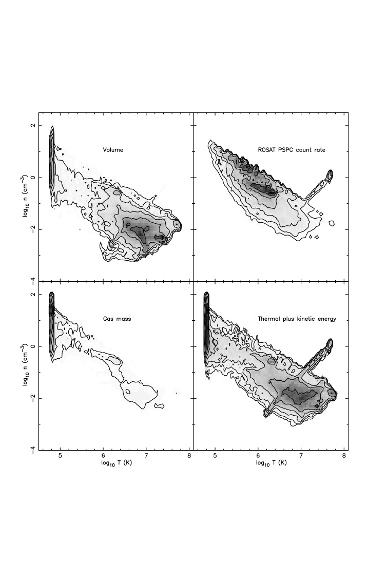
Figure 12: The distribution of volume, soft X-ray emission (ROSAT PSPC count rate), gas mass and total energy (thermal plus kinetic) as a function of gas temperature and density within the wind in model tbn1b at $t=7.5{\rm\thinspace Myr}$, binned logarithmically in temperature and density. The intensity scale has been normalised to the peak value in each panel. Contours begin at 0.1 per cent of the peak intensity, and increase in 0.5 dex intervals up to 31.6 per cent. Note that the locus of maximum X-ray emission is not the same as the locus of maximum volume, mass or energy — the X-ray emission comes from low volume filling factor gas, containing a relatively small fraction of the total mass and energy content of the galactic wind. The starburst region and the initially adiabatically expanding wind (for which $T\propto n^{2/3}$) produce the ridge running from ($\log T=7.8$, $\log n=0$) to ($\log T=6.2$, $\log n=-2.5$) in the X-ray emission and energy diagrams. The use of a minimum allowed temperature leads to the spike of material at $\log T=4.8$, which contains the majority of the total mass in the wind.

Just as the most X-ray luminous gas does not occupy much of the total wind volume, neither does it contain much of the mass and energy (either thermal or kinetic) of the wind (see Fig. 12).

Table 4: Fraction of the total wind mass, volume and energy content in the gas contributing most to the intrinsic X-ray emission (in the ROSAT PSPC band) from model tbn1b at $t=7.5{\rm\thinspace Myr}$. The most X-ray-luminous gas occupies a small fraction of the wind volume, and contains little of the mass and energy of the outflow. For example, 95 per cent of the X-ray emission is produced by only 2.4 per cent of the wind’s mass, occupying only 1.5 per cent of the total volume.

	Fraction (%)
X-ray emission	50	75	90	95
Mass	0.17	0.38	0.83	2.40
Volume	0.08	0.34	0.78	1.45
Thermal energy	0.69	2.21	5.04	7.93
Kinetic energy	0.62	2.18	5.02	10.42

The exact filling factors and mass and energy fractions depend on what we define the majority of the X-ray emission to mean. Clearly the hot gas filling most of the volume does emit soft X-rays at some level. Table 4 shows the percentage of the total gas mass, volume and energy in model tbn1b as a function of the fraction of the total unabsorbed ROSAT PSPC count rate it is responsible for, from the 50 per cent to the 95 per cent.

Even if we consider 95 per cent of all the X-ray emission we are only sampling just over 1 per cent of the wind volume, 2 per cent of the total mass and 10 per cent of the energy of the wind!

Note that although the fraction of the total mass in the X-ray dominant gas is small, there is relatively little mass in the warm and hot phases to begin with. For example, in model tbn1b only $\sim 8$ per cent of the total mass is in gas with $T\geq 10^{5.5}{\rm\thinspace K}$ (Table 3). The X-ray dominant gas in this model contains about $\sim 0.8$ per cent of the total mass, so X-ray observations would be probing of order 10 per cent of the mass of the warm and hot gas.

Table 5: Fractions of the total wind mass, volume, thermal and kinetic energy in the gas that produces the most luminous 90 per cent of the intrinsic X-ray emission in the ROSAT PSPC band (see Section 3.2.3). In all models the X-ray dominant gas is of low volume filling factor, and allows us to probe only a small fraction of the mass and energy content of the wind.

Model	$f_{\rm M}$	$\eta$ ($f_{\rm V}$)	$f_{\rm TH}$	$f_{\rm KE}$
	(%)	(%)	(%)	(%)
tbn_1	0.51	0.09	1.89	4.93
tbn1a	1.08	0.79	4.36	5.62
tbn1b	0.83	0.78	5.04	5.02
tbn_2	0.05	0.01	0.19	8.09
tbn_6	0.38	0.02	2.91	4.58
tbn_7	0.12	0.01	0.53	2.02
tbn_9	0.99	0.14	7.11	9.62
mnd_3	2.21	1.61	4.24	12.76
mnd_4	0.82	2.37	5.10	21.42
mnd_5	0.35	0.02	1.81	3.49
mnd_6	0.08	0.003	0.11	0.12
mnd_7	0.63	0.40	2.85	2.53

In all of the models we have run the gas contributing the majority of the intrinsic soft X-ray emission comes from a very small fraction of the wind. Table 5 shows the filling factors, mass and energy fractions of the gas dominating the intrinsic soft X-ray emission in all models, at a typical epoch once a full galactic wind has developed ($t=7.5{\rm\thinspace Myr}$). The lowest filling factors in Table 5, of order $10^{-2}$ per cent, may be numerical artefacts due to limited numerical resolution. This is discussed further in Section 4.

Nevertheless, it is clear that soft X-ray observations only probe a minor fraction of the wind, whether measured in terms of total volume, energy content, total mass or even mass of warm/hot gas.

3.2.4 Temperature distribution of the X-ray-emitting gas

From Fig. 12, which is typical of the temperature-density distributions found in all of these models, it is clear that gas at a wide range of temperatures and densities contributes to the X-ray emission in the ROSAT band. In Fig. 13 we show the contribution from gas at each logarithmic temperature bin to the total ROSAT PSPC count rate in models tbn_1 and mnd_3 (the default thick and thin disk galactic wind models). Even when the effect of realistic intervening absorption is included the PSPC would detect photons from a very wide range of gas temperatures.

Figure 13: The contribution from gas at each logarithmic temperature bin to the total ROSAT PSPC count rate in models tbn_1 and mnd_3 at $t=7.5{\rm\thinspace Myr}$, assuming no absorption (solid line) and $\hbox{$N_{\rm H}$}=4\times 10^{20}\hbox{${\rm\thinspace cm}^{-2}\,$}$ (dashed line). A very wide range of gas temperatures is responsible for the emission that would be detected by the ROSAT PSPC, even allowing for a realistic amount of absorption.

Figure 14: Intrinsic X-ray spectra for models tbn_1 (top) and mnd_3 (bottom) at $t=7.5{\rm\thinspace Myr}$, shown in comparison to the X-ray spectrum for a hot plasma of temperature $kT=0.5{\rm\thinspace keV}$ (bottom panel, similar to the temperature of the hot gas in starburst galaxies inferred from X-ray observations). The dotted lines show the same spectra after absorption by a hydrogen column of $\hbox{$N_{\rm H}$}=4\times 10^{20}\hbox{${\rm\thinspace cm}^{-2}\,$}$ (equivalent to the Galactic hydrogen column towards M82).

Is this consistent with existing X-ray data on the hot gas in galactic winds? As a first-order approximation to a characteristic X-ray temperature for these models we have calculated the average gas temperature $T_{\rm PSPC}$, which has been weighted by the ROSAT PSPC count rate (see Table 6). This assumes no absorption, or that given an observed X-ray spectrum we could correct for any absorption to obtain the true temperature distribution of the emitting gas.

These temperatures range from $T_{\rm PSPC}=0.08{\rm\thinspace keV}$ to $0.55{\rm\thinspace keV}$, similar if slightly lower than single temperature fits to ROSAT PSPC spectra of galactic winds. For example, Strickland et al. (1997) find best fitting temperatures ranging between $0.3$ to $0.7{\rm\thinspace keV}$ in M82’s wind, and Dahlem et al. (1998) find $kT\approx 0.1$ to $0.7{\rm\thinspace keV}$ in NGC 253’s wind. Note that the characteristic temperatures in Table 6 are not the result of fitting spectral models to observed spectra. Nevertheless, they are in broad agreement with the observed characteristic soft X-ray temperatures of galactic winds.

Although fitting simple spectral models (such as one or two temperature thermal plasma models) to simulated ROSAT or ASCA X-ray spectra from these models does give statistically good fits (as we shall show in Paper II), the derived plasma properties are misleading. We urge caution in interpreting spectra of hot gas in starburst galaxies, observed with either the preceding generation of X-ray telescopes (ROSAT or ASCA) or the latest generation (Chandra or XMM).

Very broad-band sensitive X-ray spectroscopy of the hot gas in these outflows should show more evidence of the complex temperature structure than current ROSAT or ASCA spectroscopy (where the existing broad-band coverage is compromised by source confusion and limited sensitivity). The simulated X-ray spectra for models tbn_1 and mnd_3 at $t=7.5{\rm\thinspace Myr}$ are shown in Fig. 14. Note that both are softer and harder than the spectrum of a $kT=0.5{\rm\thinspace keV}$ thermal plasma, reflecting the wide range of temperatures in the gas in these winds.

3.3 Physical origin of the soft X-ray emission

As discussed in Section 1 the origin and properties of the X-ray emitting gas in galactic winds is unclear. S94 had concluded that the majority of the soft X-ray emission in their four models came from disk and halo gas shock-heated by the wind. Recently D’Ercole & Brighenti (1999) argued that the soft X-ray emission in these models was not shock-heated disk or halo gas, but was from warm gas in the numerically broadened interfaces (i.e. artificially smoothed-out contact discontinuities) between cool dense gas and the hot wind.

In all likelihood a mixture of these two effects are responsible for the X-ray emission in these previous models, but it is very difficult to separate the two effects. Regions of ambient ISM shock-heated by the wind are also unavoidably interfaces between dense cool gas and hot tenuous gas, which will be artificially smoothed out over a number of computational cells (the exact number of which depend on the hydrodynamical scheme used. See Fryxell, Müller & Arnett [1991] for a comparison of different codes, which shows PPM-based codes that S94 and ourselves have used in a favorable light!).

Without performing much higher resolution simulations it is difficult to assess the relative significance of these two effects. See Section 4 for a more detailed discussion of the effect of numerical resolution and numerical artefacts, as well as a comparison between the models we have run at increasing resolution.

To avoid a premature choice between shock-heating of clouds and the numerical broadening of contact discontinuities as the dominant source of the soft X-ray emission in these simulations, we shall refer to “the interaction of the wind with cool dense gas.” X-ray emission from such interaction regions could then come from one or more of any number of processes: In our numerical simulations shock-heating and numerically broadened contact discontinuities, and in reality shock-heating, conductive or photo-evaporative interfaces, or turbulent mixing layers (Begelman & Fabian 1990).

If we pick out the most X-ray luminous regions within the wind, i.e. those regions responsible for the most luminous 90 per cent of the soft X-ray emission, we can find the physical origin of this emission. As we have run a wider range of models than S94 or D’Ercole & Brighenti (1999), and have included mass-loading (another process leading to soft X-ray emission), this exercise is of some interest.

We have already shown above that the soft X-ray emission comes from low filling factor gas, $\eta\sim 10^{-2}$ to $\sim 2$ per cent. We find that in all the models interaction regions (as defined above) are responsible for some, and in a few cases, all of the soft X-ray emission.

It is important to note that such interface regions do not always dominate the X-ray emission. We provide a qualitative description of which regions within the wind are responsible for the most luminous 90 per cent of the soft X-ray emission in Table 6.

Table 6: Average gas temperature in each of the models at $t=7.5{\rm\thinspace Myr}$ (weighted by ROSAT PSPC count rate, and ignoring absorption), and a qualitative description of what region the majority of the soft X-ray emission originates in.

Model	$T_{\rm PSPC}$	SBa	FWb	IRc		SHd
	(${\rm\thinspace keV}$)			w/d	w/c
tbn_1	$0.09^{+0.20}_{-0.04}$			yes	yes
tbn1a	$0.11^{+0.26}_{-0.05}$			yes	yes
tbn1b	$0.13^{+0.27}_{-0.06}$			yes	yes
tbn_2	$0.07^{+0.15}_{-0.03}$			yes	yes
tbn_6	$0.21^{+0.27}_{-0.14}$	yes		yes
tbn_7	$0.08^{+0.24}_{-0.03}$			yes	yes
tbn_9	$0.16^{+0.21}_{-0.09}$			yes	yes
mnd_3	$0.44^{+0.89}_{-0.33}$	yes	yes	yes	yes	yes
mnd_4	$0.35^{+0.42}_{-0.20}$	yes		yes	yes	yes
mnd_5	$0.55^{+0.23}_{-0.25}$	yes	yes	yes
mnd_6	$0.14^{+0.65}_{-0.10}$			yes
mnd_7	$0.19^{+0.40}_{-0.10}$	yes		yes

^a The starburst region.
^b The freely expanding wind of SN and stellar wind ejecta.
^c Interface regions, either between the wind and the ISM of the galactic disk (w/d) or between the wind and clumps of disk ISM entrained into the wind, such as superbubble shell fragments (w/c).
^d Shocked halo gas.

In the mass loaded models tbn_6, mnd_5 & mnd_7 the starburst region itself is a source of significant X-ray emission in the ROSAT band. This is easily understandable in the centrally mass-loaded models tbn_6 & mnd_5, where the central gas densities in the starburst region are an order of magnitude higher due to the additional mass injection and lower outflow velocity.

Without additional mass loading we would not normally expect the starburst region or free wind regions to be significant sources of X-ray emission, due to the low density (cf. CC). Nevertheless, the total X-ray luminosities of models mnd_3 & mnd_4 are so low (see Table 3 or Fig. 10) that these regions are counted as being X-ray dominant. Shocked halo gas is also important in these two models. The thickness of the shell of swept-up and shocked halo gas is large enough that there is no problem of unresolved contact discontinuities, as this shell is very well resolved in all the models. These models are so X-ray underluminous compared to M82 (see Table 3 or Fig. 10) that it is unlikely they are good models of M82’s wind itself.

When interface regions and shock-heated halo gas dominate the soft X-ray emission of galactic winds, abundance determinations based on X-ray spectroscopy will reflect the metallicity of the ambient disk and halo ISM to a significant degree. This is the same conclusion as reached by D’Ercole & Brighenti (1999). As a result it seems unlikely that we can directly probe the metal-enriched gas in these winds with X-ray observations, which will make it difficult to measure the metal ejection efficiency of such outflows directly.

Figure 15: The energy content of the wind in model tbn_1 as a function of time. Each of the three panels show the total (thermal plus kinetic energy, solid line), thermal (dashed line) and kinetic energy (dotted line) content of the wind as fractions of the total energy injected into the wind by the starburst. The three panels show the energy fractions within the entire wind, energy fractions of the wind within the plane of the galaxy ($|z|\leq 1.5{\rm\thinspace kpc}$), and energy fractions of the wind within the halo ($|z|>1.5{\rm\thinspace kpc}$). Initially dominated by thermal energy, post-blowout kinetic energy dominates the energy budget of the wind. Note that the wind is an efficient mechanism of transporting energy into the halo.

3.4 Wind energy and mass transport

The distribution of thermal and kinetic energy within conventional wind-blown bubbles and superbubbles has been discussed in the literature (see Mac Low & McCray [1988] and Weaver et al. [1997]), but the energy distribution within galactic winds has not been addressed until now. As galactic winds are, by definition, bulk outflows, their “energy budget” can differ substantially from the energy distribution within superbubbles.

In what form (i.e. thermal or kinetic) is the energy within the wind stored, in which gas phases, and does this depend on time, position within the wind and on the starburst or ISM? What fraction of the wind’s energy is transferred to the swept-up ISM? Which, if any, components of the wind have sufficient energy to escape the host galaxy completely? How efficient is the wind at transporting energy into the IGM?

The answer to the final question has important cosmological consequences. Galactic winds may be important for the heating of the ICM in galaxy groups and clusters (e.g. Ponman et al. 1999) and the IGM, but without knowing what fraction of the total wind energy budget can be observed in a particular wave band (e.g. soft X-ray emission, or observations of the optical emission line gas) it is difficult to assess the impact of galactic wind heating.

3.4.1 Wind energy budget and energy transport

In the standard model of a wind-blown bubble or superbubble (Weaver et al. 1977) expanding into a uniform density medium, the majority of the energy is in the thermal energy of the shocked wind region. Of the total mechanical energy injected, $\sim 45$ per cent is thermal energy in the hot shocked wind, $\sim 20$ per cent is in the form of the kinetic energy in the cool dense shell and the majority of the remaining $\sim 35$ per cent has been radiated away, primarily from the shell.

We find that blowout of the superbubble from the disk changes the energy balance of a galactic wind, from being dominated by thermal energy, to being dominated by kinetic energy (Fig. 15). In the thick disk models this can clearly be seen occurring at $t\sim 3{\rm\thinspace Myr}$. Blowout in our thin disk models is almost instantaneous, and they become kinetic energy dominated within $\sim 0.5{\rm\thinspace Myr}$.

Decomposing the energy budget into disk ($|z|\leq 1.5{\rm\thinspace kpc}$) and halo ($|z|>1.5{\rm\thinspace kpc}$) components reveals that invariably the majority of the energy injected by the starburst is transported out of the disk and into the halo (a single example using model tbn_1 is shown in Fig. 15). The total energy within the disk remains approximately constant after $t\sim 5{\rm\thinspace Myr}$, but this is a decreasing fraction of the total energy injected by the starburst.

In superbubbles the thermal energy is in predominantly in the hot ($T\geq 10^{6}{\rm\thinspace K}$) bubble interior, and the majority of the kinetic energy is in the cool ($T\sim 10^{4}{\rm\thinspace K}$) dense shell. In what temperature gas is the energy of a galactic wind stored?

Figure 16: Temperature distributions of thermal (solid line) and kinetic (dashed line) energy in model tbn1b at $t=7.5{\rm\thinspace Myr}$. The three panels show the energy within the entire wind, energy within wind material still in the plane of the galaxy ($|z|\leq 1.5{\rm\thinspace kpc}$), and the energy of the wind in the halo ($|z|>1.5{\rm\thinspace kpc}$) as a function of gas temperature. The majority of the thermal and kinetic energy of the wind is in hot, $kT\sim 0.1$ to $2.0{\rm\thinspace keV}$, gas expanding out into the halo.

In most of the models the majority of both the thermal and kinetic energy outside the plane of the galaxy ($|z|>1.5{\rm\thinspace kpc}$) is in hot gas ($6.5\leq\log T({\rm\thinspace K})\leq 7.5$), with relatively little thermal or kinetic energy in cool gas ($4.5\leq\log T({\rm\thinspace K})\leq 5.5$). This can be seen in Fig. 16, which shows the temperature distribution of the thermal and kinetic energy, over the entire wind and decomposed into disk and halo components, from model tbn1b. Table 3 gives the fractions of the total thermal or kinetic energy in the warm and hot phases of the wind in all the models.

It is interesting to note that a large fraction of the total energy of the wind is in gas that can, in principle, be probed with X-ray absorption line studies, where the relative dominance of denser X-ray emitting gas is reduced. Such absorption line studies would require bright X-ray sources in the background behind a galactic wind, and a combination of high sensitivity and spectral and spatial resolution.

In the centrally mass-loaded thick disk model tbn_6, there is very little hot gas ($6.5\leq\log T({\rm\thinspace K})\leq 7.5$). Instead, the thermal energy is predominantly in warm gas ($5.5\leq\log T({\rm\thinspace K})\leq 6.5$), while the kinetic energy of the wind is evenly spread between warm and cool gas.

Distributed mass-loading (models tbn_9 & mnd_7) differs from central mass-loading in not having such an strong effect on the energy-temperature distributions, and these models are quite similar to the non-mass-loaded models in terms of energetics.

In the weak starburst models, such as tbn_2 and mnd_4, thermal energy begins to dominate the total energy budget again after $t\sim 7.5{\rm\thinspace Myr}$. This is due to the thermal energy of the halo gas swept-up being a significant fraction of the total energy injected by the starburst in these models. In more powerful starburst models the energy content of the disk and halo ISM overrun by the wind is insignificant.

In all models the wind is efficient at transporting energy out of the plane of the galaxy, and as the winds are generally inefficient at radiating this energy away, galactic winds can in principle be good sources of heating for the IGM.

Figure 17: Wind mass as a function of time in models tbn_1 and mnd_3 (solid line), compared to the total mass of gas injected by the starburst (dotted line). The wind mass within the plane of the galaxy ($|z|\leq 1.5{\rm\thinspace kpc}$, dashed line) and above the plane ($|z|>1.5{\rm\thinspace kpc}$, dot-dashed line) are also shown. The mass of enriched material injected by the starburst ($M_{\rm inj}$) is always small compared to the mass of disk and halo gas swept-up by the wind. Note that the majority of the gas in the “wind” remains in the plane of the galaxy — galactic winds are relatively inefficient at removing gas from the galaxy.

3.4.2 Mass transport and ejection

Although the starburst can sweep up and shock large masses of ambient gas ($\mathrel{\hbox to0.0pt{\lower 3.0pt\hbox{$\sim$}\hss}\raise 2.0pt\hbox{$<$}}10^{2}\times$ the total mass of SN ejecta), most of this mass is in, and remains in the plane of the galaxy (see Fig. 17). Only a small fraction of the total mass can be found at heights above $z=1.5{\rm\thinspace kpc}$ from the plane. Galactic winds of power similar to M82’s are inefficient at transporting gas out of the plane of the galaxy.

Note that the total mass of metal-enriched gas injected by the starburst is significantly smaller than the total mass of wind material that is transported out of the disk. If all of mass associated with wind that is transported out of the disk were to make its way into the IGM, then on average gas injected into the IGM by galactic winds would not be highly metal enriched.

We cannot quantitatively assess the long term fate of the material in our simulations, given the necessarily limited spatial and temporal domain of these high resolution simulations. We can quantify what fraction of the mass of the wind currently has energy sufficient to escape the gravitational potential of the galaxy at any particular epoch. The distribution of gas mass as a function of temperature and velocity in model tbn1b at $t=7.5{\rm\thinspace Myr}$ is shown in Fig. 18. Several broad conclusions can be drawn from this figure:

1. Most of the wind’s mass is in cool gas, expanding at $v\mathrel{\hbox to0.0pt{\lower 3.0pt\hbox{$\sim$}\hss}\raise 2.0pt\hbox{$<$}}100\hbox{${\rm\thinspace km}{\rm\thinspace s}^{-1}\,$}$. This represents the slow expansion of the wind within the plane of the galaxy, where the majority of the mass is swept-up.

2. Assuming conservatively that the escape velocity $v_{\rm esc}$ from M82 is $v_{\rm esc}\sim 3\times v_{\rm rot}\sim 390\hbox{${\rm\thinspace km}{\rm\thinspace s}^{-1}\,$}$ (see for example the arguments in Heckman et al. 1999, and M82’s rotation curve in Fig. 1), then only gas above and the right of the dashed line in Fig. 18 currently has sufficient total energy to escape the galaxy. This gas is only 8.0 per cent ($\sim 4\times 10^{7}\hbox{$\thinspace{\rm M}_{\odot}$}$) of the total mass associated with the wind.

3. Interactions between the hot, energetic SN-ejecta phases of the wind and the ambient ISM has swept-up and accelerated $\sim 6\times 10^{6}\hbox{$\thinspace{\rm M}_{\odot}$}$ of cool gas ($T\mathrel{\hbox to0.0pt{\lower 3.0pt\hbox{$\sim$}\hss}\raise 2.0pt\hbox{$<$}}10^{5}{\rm\thinspace K}$) up to velocities in the range $400\leq v\mathrel{\hbox to0.0pt{\lower 3.0pt\hbox{$\sim$}\hss}\raise 2.0pt\hbox{$<$}}1000\hbox{${\rm\thinspace km}{\rm\thinspace s}^{-1}\,$}$.

4. The concentration of mass at $\log T\sim 4.8$ is due to minimum temperature allowed in these simulations. The distribution and dynamics of mass at temperatures lower than this limit is unknown, so the results above may overestimate the mass of gas with energy sufficient to escape. Note that even these high resolution simulations ($\Delta x=4.9{\rm\thinspace pc}$) do not have the numerical resolution necessary to resolve the structure and dynamics of gas cooler than this limit (see the discussion in Section 4.3), so there is little point in simulations with lower temperature limits that do not have significantly enhanced numerical resolution.

5. Using the temperature of the X-ray-emitting gas in starbursts to assess if this gas can escape the host galaxy (the so-called “escape temperature,” e.g. Wang et al. 1995; Martin 1999) will underestimate the mass of gas that can escape, as it neglects the motion of the hot gas. As discussed in Section 3.4.1, the majority of the energy in a galactic wind is in the kinetic energy of hot gas.

6. Assessing what mass of gas can escape a galaxy in the long term, based on some measure of gas energy or velocity at a particular epoch, seems extremely difficult. As the wind evolves the hot energetic gas within it will continue to entrain and accelerate cold gas. A major unknown is the effect of any halo medium (as assumed in these simulations), which acts to impeded and decelerate the wind’s expansion. Given a dense enough halo environment none of the material in a galactic wind might escape into the IGM. Treating this problem numerically is challenging, given it requires high numerical resolution to resolve the interaction between cloud and wind, as well as including the physics important to wind/cloud interactions (e.g. hydrodynamic stripping of clouds, thermal conduction, maybe even magnetic fields?).

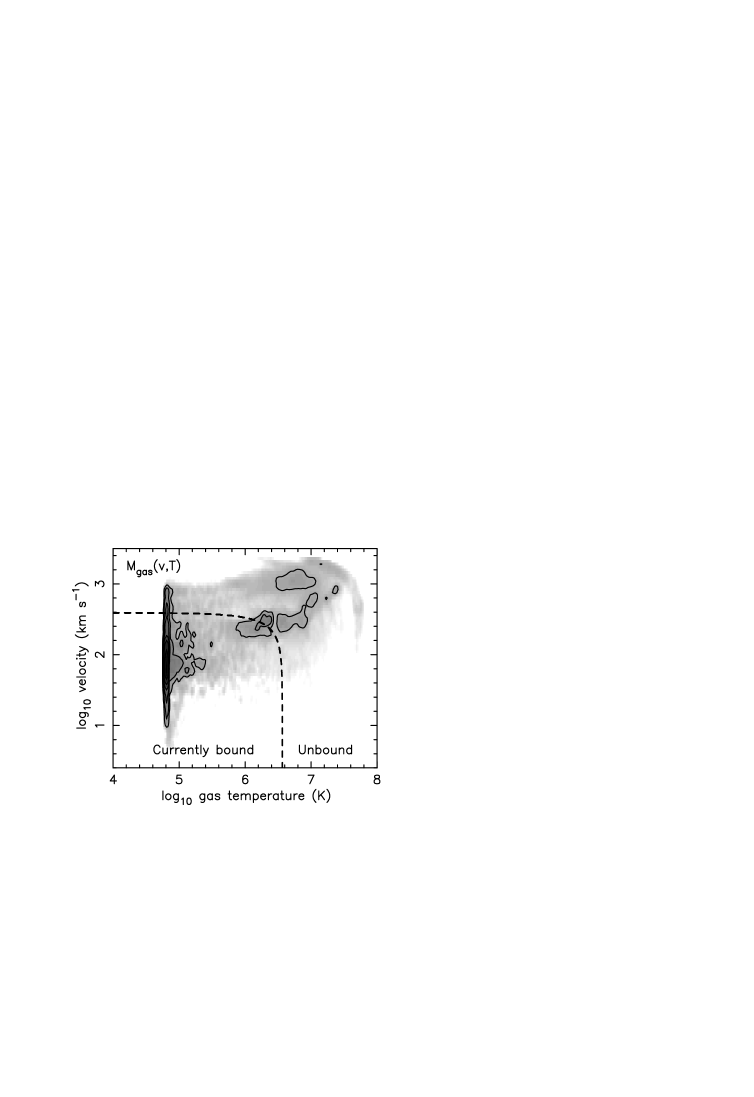
Figure 18: Mass in model tbn1b at $t=7.5{\rm\thinspace Myr}$, as a function of gas temperature and velocity. Gas above and to the right of the dashed line currently has sufficient total energy to escape the galaxy entirely, based on an escape velocity for M82 of $v_{\rm esc}=390\hbox{${\rm\thinspace km}{\rm\thinspace s}^{-1}\,$}$. Only a mass of $4\times 10^{7}\hbox{$\thinspace{\rm M}_{\odot}$}$ out of a total gas mass of $5\times 10^{8}\hbox{$\thinspace{\rm M}_{\odot}$}$ is unbound. A logarithmic intensity scale has been used to display both the cool gas dominating the total mass and the hot but tenuous energetic gas.

To summarise: (a) the mass of gas that can escape the galaxy in a starburst-driven wind is low (perhaps a few times $10^{7}\hbox{$\thinspace{\rm M}_{\odot}$}$ in a moderate starburst such as M82’s), and (b) winds are inefficient at transporting the ISM out of galaxies. These results are qualitatively consistent with those of Mac Low & Ferrara (1999) or D’Ercole & Brighenti (1999), although the outflows we have considered are 2.0 – 3.5 orders of magnitude more powerful than the winds of those authors.

4 Physical and numerical limitations

A very important aspect of any numerical hydrodynamical simulation is the degree to which the finite amount of physics included and numerical limitations (in particular finite resolution) influence the results. Understanding these effects is difficult for even the specialist, let alone for the general astronomer.

We think it is important for readers to understand the basic problems that can and do affect these and other hydrodynamical simulations. Without an understanding the limitations of a simulation it is difficult to judge what results are real and what are not. We shall discuss qualitatively the effect and importance of some of the physics that is not included in these simulations. Numerical artefacts, in particular related to resolution and numerical diffusion, are then discussed in some detail. Finally we present a comparison between three models designed to study how the simulated properties of the hot gas in galactic winds varies as we increase the numerical resolution.

4.1 Missing physics

4.1.1 Using effective instead of true gravitational potentials

The use of an effective potential $\Phi_{\rm eff}$ and the resulting effective gravity ${\bf g_{\rm eff}}$ to maintain the ISM in hydrostatic equilibrium are artefacts of a 2-D approach. A 3-dimensional code would incorporate the azimuthal velocity component without altering the gravitational field. 3-D simulations would require significant increases in terms of computation resources and code development, and are difficult to justify given that the potential scientific return of 2-D simulations has barely been tapped.

The use of a centrifugal potential means that the gravitational force felt by material within the galactic wind will be different from the true gravitational force it should feel. Put another way, the effective gravitational force in these simulations has been tuned to hold the ISM in its initial distribution given the assumption that at any position ($r$,$z$) its rotational velocity $v_{\phi}$ around the $z$-axis and hence angular momentum is known a priori. The problem is how to treat the material within the galactic wind, given that it is a mixture of material flowing outward from the central starburst region and ambient ISM swept-up and entrained into the flow. Hot gas from the starburst region itself can be presumed to have almost zero angular momentum, given its origin at the centre of the galaxy and the violent dynamics of the gas. As it flows radially and vertically outward in these 2-D simulations it feels the effective, i.e. modified by assumed rotation, gravitational force, whereas it should feel only the true gravitational force.

What effect does this have on the dynamics of the material within the wind? The effect on the very energetic free wind or shocked wind gas is negligible, as the terminal velocity of this gas is $v_{\infty}\sim 3000\hbox{${\rm\thinspace km}{\rm\thinspace s}^{-1}\,$}$, so it hardly feels the gravitational field of the galaxy. The main area where problems may arise is that the dynamics and long term evolution (over 100s of Myr) of the dense disk material dragged out of the disk and entrained into the flow (and which is assumed to be associated with the optical emission lines observed in local starbursts such as M82) may well be distorted, given that typical velocities for this gas are only several hundred kilometres per second.

As a very rough estimate of the magnitude of the force required to significantly affect the dynamics of material within the galactic wind, a final velocity of $500\hbox{${\rm\thinspace km}{\rm\thinspace s}^{-1}\,$}$ (a velocity slightly greater than the escape velocity and also significant in terms of the dynamics and morphology of the denser gas within the wind) after $10{\rm\thinspace Myr}$ of constant acceleration requires an acceleration of $\approx 1.5\times 10^{-7}{\rm\thinspace cm}\thinspace{\rm s}^{-2}$. As the difference between the true and effective gravitational fields for the thick disk ISM model is typically a tenth of this value, we can conclude that the use of an effective gravitational field does not lead to a major distortion of the wind dynamics over the time-scales of the simulations we are interested in.

4.1.2 Non-ionisation equilibrium

The hot plasma emissivities used to calculate the radiative cooling and X-ray emission from these models assume the gas is in collisional ionisation equilibrium (CIE).

For a suddenly heated plasma, the time required to reach ionisation equilibrium is approximately $t_{\rm ieq}\approx 0.03n_{\rm e}^{-1}{\rm\thinspace Myr}$ (Masai 1994) for a range of the important elements. The density and temperature structure within the wind are complex, but typical electron densities in the gas dominating the X-ray emission are of order $n_{\rm e}\sim 0.3\hbox{${\rm\thinspace cm}^{-3}\,$}$, implying an ionisation time-scale of $t_{\rm ieq}\sim 0.1{\rm\thinspace Myr}$. Although much shorter than the typical age of the wind, $t\sim 10{\rm\thinspace Myr}$, the complex dynamical state within the wind probably means it is rare that the conditions of any parcel of gas remain unchanged for this amount of time. For example, gas returned to the ISM by a SN in the starburst region is shocked within the starburst region to $T\sim 10^{8}{\rm\thinspace K}$, then flows out of the starburst region in a $v\sim 3000\hbox{${\rm\thinspace km}{\rm\thinspace s}^{-1}\,$}$ wind which rapidly adiabatically cools, before passing through the reverse shock after $\mathrel{\hbox to0.0pt{\lower 3.0pt\hbox{$\sim$}\hss}\raise 2.0pt\hbox{$<$}}1{\rm\thinspace Myr}$ and being reheated to $T\sim 10^{8}{\rm\thinspace K}$.

Much of the soft X-ray emission within a galactic wind will be due to initially cool gas incorporated into the wind, e.g. swept up and shock heated ISM, cool gas mixed into the hot wind by conduction or mass-loading and instabilities (see Section 3.3). The ionisation state of this gas will lag behind its temperature rise, as discussed by Weaver et al. (1977). Metal ions that in CIE contribute significantly to the X-ray emission of plasmas with $T\sim 10^{6}{\rm\thinspace K}$ will in practice be under-ionised. In general then the true X-ray luminosity will be less than that obtained assuming CIE.

For a rapidly cooling plasma, for example the adiabatically expanding free wind or some similar region of expansion, the gas will be over-ionised with respect to its thermal temperature. The emissivity of this gas will be less than that of a gas in CIE.

As a result of the complex ionisation histories of the gas within the wind, it is difficult to quantify how non-ionisation equilibrium (NIE) effects would alter the properties of the wind from the CIE case we assume. Calculating the ionisation state of the gas in these simulations would require tracking the history of individual parcels of gas, and would be prohibitively expensive computationally.

Given that the majority of observational analysis of real X-ray spectra assumes CIE in using the Raymond-Smith or MEKAL plasma codes, assuming CIE in creating artificial X-ray spectra does not seem too unrealistic. Systematic biases in standard X-ray spectral fitting discovered in studying the artificial X-ray observations of these wind simulations will only underestimate the true biases of fitting complex, NIE X-ray spectra with simple CIE spectral models.

4.1.3 Magnetic fields and cosmic rays

These simulations, along with the previous work of TI, TB, S94, S96 & Tenorio-Tagle & Muñoz-Tuñón (1997), ignore both cosmic rays and magnetic fields, instead focusing on a totally hydrodynamic model of galactic winds. One of the aims of this work is to see if such pressure-driven winds can reproduce the observed properties (primarily based on X-ray observations) of the best studied galactic wind in M82.

Magnetic fields and cosmic rays are known be present within the wind, but studying them is difficult and the results somewhat uncertain. Magnetic fields may be important in galactic winds over large and/or small scales. Large scale fields (over 100s to 1000s of parsecs) could potentially alter the general dynamics and expansion of the wind, for example confining its expansion in the plane of the galaxy or maybe acting to collimate it (see Sections 3.1.3 & 3.1.4). Even if magnetic fields are not important on such large scales, any smaller scale fields associated with the clouds and clumps of ambient ISM entrained into these winds could well be important. Such small scale fields might alter or inhibit the hydrodynamical stripping or conductive evaporation of these clouds, and hence affect the X-ray emission from galactic winds.

We can qualitatively assess the importance of large scale magnetic fields and of cosmic rays, relative to purely hydrodynamical processes, through comparison between the gas properties in our simulations and the existing observational data (summarised below):

1. Seaquist & Odegard (1991) estimate the total energy injection rate into the halo in the form of relativistic particles is $\mathrel{\hbox to0.0pt{\lower 3.0pt\hbox{$\sim$}\hss}\raise 2.0pt\hbox{$<$}}10^{40}\hbox{${\rm\thinspace erg}{\rm\thinspace s}^{-1}\,$}$. Compared to the mechanical energy injection rate from the starburst in these simulations of typically $\sim 10^{42}\hbox{${\rm\thinspace erg}{\rm\thinspace s}^{-1}\,$}$, cosmic rays are energetically unimportant in the halo. Cosmic rays also are unlikely to be an important source of non-thermal X-ray emission from the halo (but might be important within the starburst region itself, e.g. Moran & Lehnert 1997).

2. Klein et al. (1988) estimate a magnetic field strength of $B\sim 50\mu G$ within the central $650\times 200{\rm\thinspace pc}$ starburst region, based on the assumption of equipartition.

3. A rotation measure analysis by Reuter et al. (1994) gives a more direct estimate of the field strength $B\sim 10\mu G$ (modulo uncertainties in the column density of ionised gas), at one position at the periphery of the main ${\rm H}\alpha$ emission, about $1{\rm\thinspace kpc}$ to the south west of the nucleus.

Are fields of this range in strength dynamically important? Could such high field strengths in the starburst region constrict and confine the expansion of the wind in the plane of the galaxy? Comparing magnetic pressure ($P_{\rm B}=B^{2}/8\pi$) to thermal and ram pressures within the wind provides a simple basis for comparison. A magnetic field strength of $B=50\mu G$ corresponds to $P_{\rm B}/k\sim 8\times 10^{5}{\rm\thinspace K}\hbox{${\rm\thinspace cm}^{-3}\,$}$, a field of $B=10\mu G$ to $P_{\rm B}/k\sim 3\times 10^{4}{\rm\thinspace K}\hbox{${\rm\thinspace cm}^{-3}\,$}$.

In the plane of the galaxy, where confinement of the wind’s expansion is such a problem, typical thermal and ram pressures are $P_{\rm TH}/k\sim 2\times 10^{6}{\rm\thinspace K}\hbox{${\rm\thinspace cm}^{-3}\,$}$ and $P_{\rm RAM}/k\sim 7\times 10^{6}{\rm\thinspace K}\hbox{${\rm\thinspace cm}^{-3}\,$}$ for the powerful starbursts we have simulated (e.g. tbn1b, mnd_3). At a height of $z=1{\rm\thinspace kpc}$ above the plane of the galaxy pressures are typically lower ($P_{\rm TH}/k\sim 10^{6}{\rm\thinspace K}\hbox{${\rm\thinspace cm}^{-3}\,$}$, $P_{\rm RAM}/k\sim 2\times 10^{6}{\rm\thinspace K}\hbox{${\rm\thinspace cm}^{-3}\,$}$), but in some locations ram pressures can reach exceedingly high values ($P_{\rm RAM}/k\mathrel{\hbox to0.0pt{\lower 3.0pt\hbox{$\sim$}\hss}\raise 2.0pt\hbox{$>$}}2\times 10^{7}{\rm\thinspace K}\hbox{${\rm\thinspace cm}^{-3}\,$}$).

Drawing some tentative conclusions from this, it appears that:

1. The estimated magnetic field strength of $B\sim 50\mu G$ within M82’s starburst region, although high by the standards of normal galactic magnetic fields, is still somewhat lower than that required to make the magnetic field dynamically important in confining the expansion of the wind within the plane of the galaxy.

2. If large scale field strengths are typically $B\mathrel{\hbox to0.0pt{\lower 3.0pt\hbox{$\sim$}\hss}\raise 2.0pt\hbox{$<$}}10\mu G$ within the wind, then they are dynamically unimportant.

3. However, if stronger large scale fields, of order $B\sim 50\mu G$, exist throughout the entire wind then the energy in such magnetic fields would be comparable to, or greater than, the thermal and kinetic energy of the hot gas.

Hence it does not appear that large scale magnetic fields are dynamically important for understanding this class of galactic-scale outflows. The question of the influence and importance of smaller scale fields in the interaction between the wind and clouds embedded within it remains open.

4.1.4 Thermal conduction

In common with most previous simulations we ignore thermal conduction, as it difficult to include in multidimensional hydrodynamic schemes and computationally expensive. In the standard wind-blown bubble model of Weaver et al. (1977) evaporation of the cold bubble shell by thermal conduction is the dominant source of mass in the hot bubble interior, increasing its density by approximately an order of magnitude. As a result, the effects of thermal conduction on the X-ray emission from wind-blown bubbles and superbubbles are very important.

In galactic winds thermal conduction is expected to be important in regions where there are reservoirs of dense cool gas in close proximity to hot gas, such as the interface between the shocked wind and the disk within the plane of the galaxy, or in the vicinity of superbubble shell fragments within the halo.

One effect of thermal conduction is to increase the density of the hot X-ray-emitting gas, in a similar manner to mass loading. Indeed, Mac Low & Ferrara (1999) add additional mass into their simulations of very weak winds in dwarf galaxies to approximate the effects of conduction in a manner similar to our method of central mass loading. Our mass-loading can be considered as a rough approximation to the effects of both hydrodynamical mass-loading and thermal conduction, although a rigorous treatment of thermal conduction is beyond the scope of this work.

Thermal conduction, unless inhibited in some manner, might also totally evaporate the cool dense clumps and clouds seen in our simulations. As described in Ferrara & Shchekinov (1993), clouds smaller than the Field length (Field 1965) will suffer rapid conduction-driven evaporation, loosing a very substantial fraction of their mass before achieving a semi-stable configuration. For the range of temperatures and densities found in the hot gas filling the majority of the wind’s volume in our simulations, the Field length ranges from several hundred parsecs to several kiloparsecs, so all of the clumps seen in our simulations should suffer conductive evaporation.

The net effect of conduction is difficult even to describe qualitatively. The addition of mass to the hot phases of a galactic wind will increase the X-ray emission from the wind itself, but if conduction destroys clouds totally then the net effect might be a reduction in total X-ray luminosity, given that cloud/wind interfaces appear to be such strong sources of X-ray emission in these simulations.

Very recently D’Ercole & Brighenti (1999) have performed a 2-D simulation of a starburst-driven wind in a dwarf galaxy (based approximately on the dwarf starburst NGC 1569) that includes thermal conduction. Interestingly, thermal conduction leads to an increase in the soft X-ray luminosity of this particular model by a factor of between 1 and 3 from the non-conductive case.

4.1.5 Photoionisation by the wind

These simulations assume all material within the wind is optically thin to its own radiation, i.e. there is no absorption intrinsic to the wind. This assumption is necessary to carry out these simulations, as coupled multidimensional radiation-hydrodynamic problems are exceedingly challenging to solve.

For emission from, and propagating through, the hot tenuous material of the wind (e.g. free wind, shocked wind and shocked halo regions) this assumption is reasonable. Typical columns densities of the highly ionised material that would be encountered by radiation traversing the wind are in the range $10^{19}$ – $10^{20}\hbox{${\rm\thinspace cm}^{-2}\,$}$.

In the vicinity of cool dense clouds and the walls of the outflow within the disk, column densities become more significant. Typical column densities traversing a single clump range from $\sim 5\times 10^{19}$ – $10^{21}\hbox{${\rm\thinspace cm}^{-2}\,$}$, depending on whether the line of sight crosses the tail or head of a clump and what the angle of incidence is.

The environment around these cool dense regions is the source of the majority of soft X-ray emission (and UV emission, which we have not discussed) from galactic winds. Photoionisation of these clouds by the energetic radiation produced through various cloud/wind interactions may well have dynamical and observational consequences. This could lead to further evaporation of the clouds, as well as to alter their ionisation state further from the collision ionisation equilibrium assumed in these calculations and in most X-ray spectral fitting.

Another important consequence of this will be a reduction in the X-ray emission escaping the wind, due to the absorption of a substantial fraction of the softest X-ray emission, produced at cloud/wind interfaces, by the clouds themselves. A column of $10^{20}\hbox{${\rm\thinspace cm}^{-2}\,$}$ (assuming Solar abundances, at it is the metals such as Carbon, Nitrogen and Oxygen that dominate the photoelectric absorption cross-section) is optically thick to radiation of energy below $E\sim 0.2{\rm\thinspace keV}$. The densest clouds, with individual columns of $\sim 10^{21}\hbox{${\rm\thinspace cm}^{-2}\,$}$ are optically thick to X-rays with energy less than $\sim 0.4{\rm\thinspace keV}$. Such a reduction in the “escaping” X-ray luminosity from the wind will bring the soft X-ray luminosities of our simulations into closer agreement with the observed soft X-ray luminosities of galactic winds (cf. Section 3.2.1).

4.2 Numerical resolution and cell size

For a structured Cartesian grid as employed in these simulations the resolution is proportional to the cell size used. The properties of an unresolved structure, e.g. the cold dense superbubble shell, will be averaged out over the computational cell, as the finite volume scheme employed ensures total mass and energy within the cell are conserved correctly. For the example of a unresolved superbubble shell, the density and thickness of the shell in the simulation will respectively be less than and greater than the true values.

In addition to affecting the absolute values of the fluid variables, finite numerical resolution can affect the dynamics of the fluid in other ways. Consider for example the fragmentation of the superbubble shell by Rayleigh-Taylor (RT) instabilities (cf. S94). The Rayleigh-Taylor instability time-scale is $\tau_{\rm RT}\propto\lambda^{1/2}$, where $\lambda$ is the wavelength. The perturbations that eventually disrupt the shell have wavelengths similar to the shell thickness, so unresolved shells are artificially stable against the RT instability, and eventually fragment into artificially large pieces.

This directly effects the dynamics and properties of the coolest gas in these simulations. Fig. 19 shows images of the logarithm of the gas number density in models tbn_1, tbn1a (which has cells half the size of those in model tbn_1) & tbn1b (cells one third the size of those in model tbn_1). It is immediately clear that the coolest densest gas in models tbn1a & tbn1b is far more structured than that in model tbn_1, and that there are many more superbubble shell fragments being dragged out with the wind.

The limitations of a finite cell size are worst for the densest, coolest gas, as it is typically found in the smallest structures. The hotter, tenuous gas, such as the thick shell of shocked halo gas or regions of shocked wind material, is on the other hand most likely to be well resolved, as it occurs in structures much larger than the cell size.

Nevertheless, poor numerical resolution of cool dense gas can affect the properties of the hot X-ray emitting gas we are primarily interested in. The main problems here are the artificial broadening of contact discontinuities between cool dense gas and hot tenuous gas, which creates regions of intermediate density warm gas that will produce significant amounts of soft X-ray emission, and numerical diffusion which further acts to increasingly broaden contact discontinuities and spread material over more cells with time.

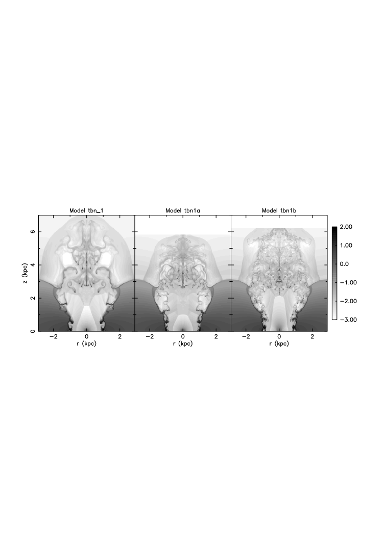
Figure 19: Wind number density distributions for models tbn_1, tbn1a and tbn1b at $t=7.5{\rm\thinspace Myr}$, shown as grey-scale images of $\log n(\hbox{${\rm\thinspace cm}^{-3}\,$})$. Model tbn1a has twice the resolution of model tbn_1, model tbn1b triple the resolution. Note the dramatic increase in the complexity of the structure of the densest gas as the resolution is increased.

4.3 Cell size vs. shell thickness

It is important to understand that the true resolution of a hydrodynamic simulation is not equal to the size of a single cell, but to the number of cells over which the code used can represent abrupt changes in the fluid variables such as shocks or contact discontinuities.

One of the great advantages of the Piecewise Parabolic Method (PPM) used by VH-1 it that it spreads out shocks over only two cells, a major advantage over many other numerical scheme which spread shocks out over 4 – 5 cells. Shocks are an integral part of galactic winds, as can be seen from the many shocks visible in the gas number density images shown in Figs. 4 – 7.

As a rough estimate of how well the densest structures in our simulations are resolved we compare the cell size to analytical estimates of the thickness of the superbubble shell before RT instabilities fragment it. A simple method of estimating the shell thickness is to use the Weaver et al. (1977) model of a constant mechanical luminosity wind blowing into a constant density medium. Using the analytical solutions presented by Weaver et al. , we can calculate the total mass in the shell and its pressure, as a function of time. Assuming the shell cools to the minimum temperature we allow on our computational grid, $T_{\rm disk}=6.5\times 10^{4}{\rm\thinspace K}$, the density of the shell follows directly from the pressure. Given the total mass of the shell and its surface area, the shell thickness follows trivially. Using the appropriate conditions that the superbubble experiences before blowout at $t\sim 3{\rm\thinspace Myr}$ in the thick disk models, the shell thickness is typically $\Delta r_{\rm sh}\sim 10{\rm\thinspace pc}$. Comparing this to the cell size in model tbn_1 ($\Delta x=14.6{\rm\thinspace pc}$), model tbn1a ($\Delta x=7.3{\rm\thinspace pc}$) and model tbn1b ($\Delta x=4.9{\rm\thinspace pc}$) shows that the superbubble shell is under-resolved, although not drastically so.

Hence the shell fragmentation process and the number and size of superbubble fragments is controlled by the resolution of these simulations.

Note that this also means that without dramatic increases in resolution there is no point in allowing gas temperatures below the minimum gas temperature of $T_{\rm disk}=6.5\times 10^{4}{\rm\thinspace K}$ we impose (see Section 2.4). A superbubble shell of temperature equivalent to the optical emission line gas observed in winds like M82’s of $T\sim 10^{4}{\rm\thinspace K}$ would be $\sim 2{\rm\thinspace pc}$ thick, and hence totally unresolved.

4.4 Numerical diffusion at contact discontinuities

As we have mentioned, numerical broadening of contact discontinuities will affect the properties of the X-ray emitting gas. In reality physical processes such as thermal conduction and turbulent mixing layers will also create layers of intermediate temperature and density gas between cool dense gas and hot tenuous wind material. The problem with numerically broadened contact discontinuities is that their width and structure (and hence the properties of any artificial X-ray emitting region) is determined directly by the numerical scheme employed, and not by real physical processes.

As discussed in Fryxell et al. (1991), contact discontinuities continue to spread diffusively without limit in many Eulerian hydrodynamical codes, as the contact region moves over the computational grid. They show that of a series of numerical methods PPM is the best at retaining sharp contact discontinuities. With the additional use of an contact discontinuity steepener algorithm, PPM spreads and maintains such discontinuities over a width on only two cells. VH-1 does not use such a contact discontinuity steepener, although the Lagrangian remap scheme used in VH-1 is believed to be better than the Eulerian PPM scheme studied by Fryxell et al. (1991) at maintaining sharp contact discontinuities without the use of a steepener (Blondin 1994).

We also employ a scheme similar to that used by Stone & Norman (1993) to reduce cooling in the region of contact discontinuities to reduce the unphysical cooling from the broadened discontinuity.

Although the efficient shock and discontinuity capturing within PPM mitigate the effects of finite numerical resolution, we can not totally remove such effects.

4.5 Increasing numerical resolution: models tbn_1, tbn1a and tbn1b

To investigate how sensitively our results depend on the numerical resolution of our models we ran three simulations using almost the same starburst and ISM parameters but successively increasing the resolution.

Models tbn_1 and tbn1a differ only in the cell size. Each computation cell in model tbn_1 representing a region $14.6{\rm\thinspace pc}\times 14.6{\rm\thinspace pc}$ in size, compared to cells of $7.3{\rm\thinspace pc}\times 7.3{\rm\thinspace pc}$ in model tbn1a. Model tbn1b has triple the resolution of model tbn_1, with cells of $4.9{\rm\thinspace pc}\times 4.9{\rm\thinspace pc}$, but differs from the other thick disk models in using a cylindrical rather than spherical starburst region.

The most dramatic differences between the three simulations is in the amount of structure visible in the densest coolest gas. For example, the number of superbubble shell fragments visible at $t=7.5{\rm\thinspace Myr}$ increases significantly and their size decreases as the resolution increases (see Fig. 19), for the reasons explained in Section. 4.2.

Otherwise the overall morphology of the wind is very similar between the different simulations, barring some minor differences in overall volume occupied by the wind.

Figure 20: The distribution of volume, X-ray flux, emission measure and mass with temperature at $t=7.5{\rm\thinspace Myr}$ in models tbn_1 (solid line), tbn1a (dashed) and tbn1b (dotted). Note the extremely close agreement between the emission measure and ROSAT count rate distributions for gas hotter than $kT\sim 0.1{\rm\thinspace keV}$. For gas cooler than this temperature the higher resolution models predict less emission.

The properties of the X-ray emitting gas, whether measured in terms of the distribution of volume, average density, emission measure or emitted X-ray flux as a function of temperature, are all very similar between the three models when measured at the same epoch (see Fig. 20 and Table 3).

Concentrating on the properties most important observationally, the emission measure and ROSAT PSPC count rates, the agreement between the different models is excellent at gas temperatures above $kT\sim 0.1{\rm\thinspace keV}$. For gas with temperatures below this, the higher resolution models predict systematically less emitting material and less X-ray flux.

This is consistent with a picture of some, although not necessarily all, of the X-ray emission from gas at these lower temperatures being due to numerically broadened contact discontinuities.

The only other significant difference between these models we have found is in the filling factors of the X-ray dominant gas (Table 5), where model tbn_1 has a much lower filling factor than models tbn1a & tbn1b. We do not believe the filling factors of the most of the other models are as dependent on numerical resolution as model tbn_1. In particular, in the thin disk models the X-ray emission is not purely from such interface regions (where numerically broadened contact discontinuities are such a problem), so increased numerical resolution should not lead to order of magnitude increases in the filling factor of the X-ray dominant gas.

The models where the properties of the X-ray dominant gas are most likely to be affected by resolution effects are models tbn_1, tbn_2, tbn_7 and mnd_6. This is based on the number of computational cells the most X-ray luminous gas covers (i.e. the gas contributing 90 per cent of the soft X-ray counts in the ROSAT band), which is much lower in these models than in any of the other models.

Comparing the intrinsic X-ray luminosities in the ROSAT $0.1$ – $2.4{\rm\thinspace keV}$ energy band as a function of time between the three models also shows progressively lower X-ray luminosity accompanies higher numerical resolution (Fig. 21). This figure probably exaggerates the importance of the variation in X-ray luminosity with resolution, as what can be measured in reality will be the count rate of the attenuated emission, where the influence of the low temperature gas so affected by numerical effects is significantly reduced. There will be much less difference between the “observable” X-ray properties of these models than in their intrinsic X-ray luminosities.

Figure 21: X-ray luminosity in the ROSAT $0.1$ – $2.4{\rm\thinspace keV}$ energy band, as function of time in models tbn_1 (solid line), tbn1a (dashed) and tbn1b (dotted). Most of the variation in X-ray luminosity is due to changes in the properties of warm gas ($kT\mathrel{\hbox to0.0pt{\lower 3.0pt\hbox{$\sim$}\hss}\raise 2.0pt\hbox{$<$}}0.1{\rm\thinspace keV}$) as the numerical resolution increases from model tbn_1 to tbn1b.

The coolest gas in these simulations is not resolved, and would require quite substantial further increases in numerical resolution to resolve if it were allowed to cool to $T\sim 10^{4}{\rm\thinspace K}$. The dramatic increase in the complexity of the structures associated with the coolest gas with increasing resolution does suggest to us that the complex filamentary structure of the optical emission line gas observed in galactic winds (cf. McKeith et al. 1995; Lehnert & Heckman 1996; Shopbell & Bland-Hawthorn 1998) will be produced as a natural consequence of these models, once they achieve the necessary resolution.

The level of variation found between these three simulations implies that in these simulations, including the other thick and thin disk models, the emission properties of the low filling factor warm gas responsible for the majority of the soft X-ray emission ($kT\mathrel{\hbox to0.0pt{\lower 3.0pt\hbox{$\sim$}\hss}\raise 2.0pt\hbox{$<$}}0.1{\rm\thinspace keV}$) are partially controlled by unresolved, numerically broadened, warm gas interfaces between cool dense gas and hotter wind material. Nevertheless, the important finding that the X-ray dominant gas has low filling factor ($\mathrel{\hbox to0.0pt{\lower 3.0pt\hbox{$\sim$}\hss}\raise 2.0pt\hbox{$<$}}2$ per cent), is likely to be robust.

Hotter gas within these winds ($kT\mathrel{\hbox to0.0pt{\lower 3.0pt\hbox{$\sim$}\hss}\raise 2.0pt\hbox{$>$}}0.1{\rm\thinspace keV}$), in particular volume filling components, seems well resolved, even in our lowest resolution simulations and therefore its properties are reasonably quantitatively correct.

5 Summary

We have performed an extensive parameter study of starburst-driven galactic winds using a high resolution 2-D hydrodynamical code, focusing on the best studied galactic wind in M82. These simulations allow us to study how the properties of galactic winds vary depending on the influence of the host galaxy’s ISM distribution, starburst strength and star formation history, and the presence or absence of additional mass-loading from clouds enveloped in the wind.

In this paper we have used this sample of twelve simulations to investigate several aspects of galactic winds that are uncertain or have previously received little attention: the origin and filling factor of the gas responsible for the observed soft X-ray emission; wind energetics and energy transport efficiencies and wind collimation and growth. In addition we have explored in detail the influence of finite numerical resolution on the results of these simulations.

The results of this study are summarised below:

5.1 Wind collimation and confinement

1. Thick ISM disks are required to reproduce the well collimated wind observed in M82. Thin disk models (e.g. Suchkov et al. 1994) have wind opening angles that are too large, $\theta\mathrel{\hbox to0.0pt{\lower 3.0pt\hbox{$\sim$}\hss}\raise 2.0pt\hbox{$>$}}90\hbox{${}^{\circ}$}$. Thick disk models, such as that used by Tomisaka & Bregman (1993), are much better collimated, with typical opening angles $\theta\sim 40\hbox{${}^{\circ}$}$, much closer to the observed value of $\theta\sim 30\hbox{${}^{\circ}$}$.

2. All the simulations, regardless of ISM distribution or star formation history, fail to confine the size of the wind in the plane of the galaxy to the observed size of roughly the size of the starburst region ($\sim 400{\rm\thinspace pc}$ in M82). The radius of the wind in the plane of the galaxy grows to between 1 – 2 kpc over the 10 Myr period covered by these simulations. The confinement of galactic winds within the plane of the galaxy remains a problem, as initially pointed out by Tenorio-Tagle & Muñoz-Tuñón (1997). There is clearly something interesting happening in the central regions of starburst galaxies, perhaps related to the existing circum-nuclear molecular rings, that must be able confine the base of the wind over time-scales of $\sim 10{\rm\thinspace Myr}$.

5.2 X-ray emission in galactic winds

1. The gas responsible for the majority of the soft X-ray emission detectable by ROSAT comes from very low filling factor ($\eta\sim 0.01$ to $2$ per cent) gas that contains very little of the total mass or energy of the wind. As a result X-ray observations with ROSAT, ASCA, Chandra or XMM will only give lower limits on the mass and energy content of galactic winds.

2. The winds in these models contain gas at a wide range of temperatures and densities. In terms of a phase description there is a phase continuum of states rather than any particular well defined characteristic temperatures or densities.

3. The majority of the wind volume in almost all of these models is filled with hot gas, covering the temperature range $10^{6.5}$ to $10^{7.5}{\rm\thinspace K}$. This gas is only a weak source of soft X-ray emission due to its low density.

4. The soft X-ray emission in these models does not come from any single well-defined temperature gas, but from a very wide range of temperatures from $T\sim 10^{5}{\rm\thinspace K}$ to $10^{8}{\rm\thinspace K}$. Fitting the resulting complex X-ray spectra with standard simple spectral models is likely to give misleading results.

5. In all of our models, regions of interaction between the hot wind and cooler denser material (originally part of the ambient ISM) give rise to a large fraction of the soft X-ray emission. In these simulations this X-ray emission can be from shock-heated ambient gas, and from the numerically broadened interfaces between cool dense and hot tenuous gas, although it is very difficult to discriminate between the two cases. In some of the models, in particular the mass-loaded models, the starburst region itself or the free wind region can be significant sources of soft X-ray emission. In the thin disk models shock-heated halo gas is also an important source of X-ray emission.

6. The primary variable affecting the soft X-ray luminosity of the galactic winds in these models is the density and distribution of the ambient, volume-filling, component of the ISM. The energy injection rate from the starburst, and mass-loading from dense clouds, do have a significant but secondary effect on the X-ray luminosity.

7. Mass-loading of the wind, either within the starburst region itself, or from clouds distributed more generally throughout the ISM, is not necessary to produce galactic winds of M82’s luminosity or characteristic soft X-ray temperature.

8. Hard X-ray emission from galactic winds is dominated by the starburst region itself. The ratio of hard X-ray to soft X-ray luminosity is typically $L_{\rm X,hard}/L_{\rm X,soft}\sim 10^{-2}$. We confirm S94’s conclusion that the hard X-ray emission from starburst galaxies is not due to thermal emission associated with the starburst-driven wind.

5.3 Wind energetics

1. Galactic winds are efficient at transporting the energy supplied by the starburst out of the plane of the galaxy. As radiative losses are low, galactic winds seem likely to be good sources of heating for the IGM and ICM. This is in contrast to their low efficiency at moving mass out of the disk of starburst galaxies.

2. The energy within galactic winds is predominantly ($\sim 60$ per cent) kinetic energy of hot gas ($10^{6.5}\leq T(K)\leq 10^{7.5}$). This is significantly different from the standard superbubble, where the majority of the energy is in the thermal energy of the hot bubble interior. The change from thermally-dominated to kinetically-dominated energetics occurs when the superbubble breaks out of the disk.

3. Hot gas also contains the majority ($\sim 60$ per cent) of the total thermal energy content of these winds. Exceptions to this rule are models with strong centralised mass-loading, where warm gas ($10^{5.5}\leq T(K)\leq 10^{6.5}$) dominates the thermal energy content.

4. The total energy content of galactic winds appears extremely difficult to measure directly: Soft X-ray observations probe only denser low filling factor gas containing relatively little ($\mathrel{\hbox to0.0pt{\lower 3.0pt\hbox{$\sim$}\hss}\raise 2.0pt\hbox{$<$}}10$ per cent) of either the total thermal or kinetic energy. Measuring the kinetic energy of the warm and hot phases is also hampered by the lack of any direct measurements of this gas’s velocity.

5.4 Concluding remarks

Our findings have major implications for the ultimate aim behind the study of galactic winds: measuring quantitatively the transport of mass, metal-enriched gas and energy out of star-forming galaxies.

These simulations measure, for the first time, the observationally important filling factor of the X-ray emitting gas. In all models, even those including different forms of mass-loading, we find that the soft X-ray emission from galactic winds comes from low filling factor ($\eta\mathrel{\hbox to0.0pt{\lower 3.0pt\hbox{$\sim$}\hss}\raise 2.0pt\hbox{$<$}}2$ per cent) gas. This gas contains only a small fraction of the mass and energy of the wind. The majority of the thermal and kinetic energy of these outflows is in a hot, volume filling, component, which is extremely difficult to probe observationally due to its low density and hence low emissivity.

We also find that galactic winds are efficient at transporting energy out of the host galaxy, primarily in the form of the kinetic energy of hot, $T\sim 10^{6.5}$ to $10^{7.5}{\rm\thinspace K}$, gas. This is an important finding, as it suggests that starburst-driven winds are a good mechanism for reheating the IGM and ICM, as required by recent observations.

In Paper II we shall present a direct comparison between the spectral properties and spatial distribution of the soft X-ray emission in these models and the existing X-ray data on M82, along with a discussion of which of these models best reproduces M82’s observed properties.

It is a pleasure to thank the referee, A. Ferrara, both for the scientific value of his comments and the punctuality of his response! We would also like to thank the numerous people whose comments on this work we have found enlightening, in particular Timothy Heckman, Martin Ward, Duncan Forbes, Trevor Ponman, Crystal Martin and Martin Norbury. DKS acknowledges financial support from a PPARC studentship, a Teaching Assistantship from the School of Physics & Astronomy at the University of Birmingham and through NASA grant NAGW 3138. IRS acknowledges support from a PPARC Advanced Fellowship.

References

- [] Allen M. L., Kronberg P. P., 1998, ApJ, 502, 218
- [] Arthur S. J., Henney, W. J, 1996, ApJ, 457, 752
- [] Begelman M. C., Fabian A. C., 1990, MNRAS, 244, 26P
- [] Bland-Hawthorn J., 1995, Publ. Astron. Soc. Aust., 12, 190
- [] Blondin J. M., 1994, The VH-1 Users Guide, University of Virginia
- [] Blondin J. M., Kallman T. R., Fryxell B. A., Taam R. E., 1990, ApJ, 356, 591
- [] Bradamante F., Matteucci F., D’Ercole A., 1998, A&A, 337, 338
- [] Bregman J. N., Schulman E., Tomisaka K., 1995, ApJ, 439, 155
- [] Calzetti D., Meurer G. R., Bohlin R. C., Garnett D. R., Kinney A. L., Leitherer C., Storchi-Bergmann T., 1997, AJ, 114, 1834
- [] Cappi M., et al. , 1999, A&A in press (astro-ph/9908312)
- [] Chevalier R. A., Clegg A. W., 1985, Nat, 317, 44 (CC)
- [] Cole S., Aragon-Salamanca A., Frenk C. S., Navarro J. F., Zepf S. E., 1994, MNRAS, 271, 781
- [] Collela P., Woodward P. R., 1984, J. Comp. Phys., 54, 174
- [] Cottrell G. A., 1977, MNRAS, 178, 577
- [] Cowie L. L., McKee C. F., Ostriker J. P., 1981, ApJ, 247, 908
- [] Dahlem M., 1997, PASP, 109, 1298
- [] Dahlem M., Heckman T. M., Fabbiano G., Lehnert M. D., Gilmore D., 1996, ApJ, 461, 724
- [] Dahlem M., Weaver K. A., Heckman T. M., 1998, ApJS, 118, 401
- [] de Gouveia Dal Pino E. M., Medina Tanco G. A., 1999, ApJ, 518, 129
- [] Dekel A., Silk J., 1986, ApJ, 303, 39
- [] Della Ceca R., Griffiths R. E., Heckman T. M., 1997, ApJ, 485, 581
- [] De Young D. S., Heckman T. M., 1994, ApJ, 431, 598
- [] D’Ercole A., Brighenti F., 1999, MNRAS, in press
- [] Fabbiano G., 1988, ApJ, 330, 672
- [] Ferrara A., Shchekinov Yu., 1993, ApJ, 417, 595
- [] Field G.B., 1965, ApJ, 142, 531
- [] Freedman, W.L. et al. , 1994, ApJ, 427, 628
- [] Fryxell B., Müller E., Arnett D., 1991, ApJ, 367, 619
- [] Godunov S. K., 1959, Mat. Sb. 47, 271
- [] González Delgado R. M., Leitherer C., Heckman T., Cerviño M., 1997, ApJ, 483, 705
- [] Gorjian V., 1996, AJ, 112, 1886
- [] Götz M., McKeith C. D., Downes D., Greve A., 1990, A&A, 240, 52
- [] Hartquist T. W., Dyson J. E., Pettini M., Smith L. J., 1986, MNRAS, 221, 715
- [] Hartquist T. W., Dyson J. E., Williams R. J. R., 1997, ApJ, 482, 182
- [] Heckman T. M., 1998, in ‘Origins’, ASP Conference Series 145, Eds. C. E. Woodward, J. M. Shull and H. A. Thronson Jr, 127
- [] Heckman T. M., Armus L., Miley G. K., 1990, ApJS, 74, 833
- [] Heckman T. M., Lehnert M. D., Armus L., 1993, in “The Environment and Evolution of Galaxies,” Eds. J. M. Shull and H. A. Thronson Jr, (Dordrect:Kluwer), 455
- [] Heckman T.M., Lehnert M.D., Strickland D.K., Armus L., 1999, submitted to ApJ
- [] Kauffman G., Guiderdoni B., White S. D. M., MNRAS, 267, 981
- [] Klein R. I., McKee C. F., Collela P., 1994, ApJ, 420, 213
- [] Klein U., Wielebinski R., Morsi H. W., 1988, A&A, 190, 41
- [] Lehnert M. D., Heckman T. M., 1996, ApJ, 462, 651
- [] Leitherer C., Heckman T. M., 1995, ApJS, 96, 9 (LH95)
- [] Leitherer C., Robert C., Drissen L., 1992, ApJ, 401, 596
- [] Loewenstein M., Mushotzky R. F., 1996, ApJ, 466, 695
- [] Lugten J. B., Watson D. M., Crawford M. K., Genzel R., 1986, ApJ, 311, L51
- [] McCarthy P. J., Heckman T., van Breugel W., 1987, AJ, 92, 264
- [] Mac Low M.-M., Ferrara A., 1999, ApJ, 513, 142
- [] Mac Low M.-M., McCray R., 1988, ApJ, 324, 776
- [] McKeith C. D., Greve A., Downes D., Prada F., 1995, A&A, 293, 703
- [] McLeod K. K., Rieke G. H., Rieke M. J., Kelly D. M., 1993 ApJ, 412, 111
- [] Martin C. L., 1999, ApJ, 513, 156
- [] Masai K., 1994, ApJ, 437, 770
- [] Meurer G. R., Heckman T. M., Leitherer C., Kinney A., Robert C., Garnett D. R., 1995, AJ, 110, 2665
- [] Mewe R., Kaastra J. S., Liedahl D. A., 1995, Legacy, 6, 16
- [] Miyamoto M., Nagai R., 1975, PASJ, 27, 533
- [] Moran E. C., Lehnert M. D., 1997, ApJ, 478, 172
- [] Morrison R., McCammmon D., 1983, ApJ, 270, 119
- [] Muxlow T. W. B., Pedlar A., Wilkinson P. N., Axon D. J., Sanders E. M., de Bruyn A. G., 1994, MNRAS, 266, 455
- [] Nakai N., Hayashi M., Handa T., Sofue Y., Hasegawa T., 1987, PASJ, 39, 685
- [] Norman C. A., Ferrara A., 1996, ApJ, 467, 280
- [] O’Connell R. W., Mangano J. J., 1978, ApJ., 221, 62
- [] O’Connell R.W., Gallagher J.S., Hunter D.A., Colley W.N. 1995, ApJ, 446, L1
- [] Pettini M., Steidel C. C., Adelburger K. L., Dickinson M., Giavalisco M., 1999, ApJ, in press (astro-ph/9908007)
- [] Ponman T. J., Cannon D. B., Navarro J. F., 1999, Nat, 397, 135
- [] Ptak A. F., 1997, Ph.D. Thesis, University of Maryland
- [] Ptak A., Serlemitsos P., Yaqoob T., Mushotzky R., Tsuru T., 1997, AJ, 113, 1286
- [] Puxley P. J., Brand P. W. J. L., Moore T. J. T., Mountain C. M., Nakai N., Yamashita T., 1989, ApJ, 345, 163
- [] Raymond J. C., Smith B. W., 1977, ApJS, 35, 419
- [] Read A. M., Ponman T. J., Strickland D. K., 1997, MNRAS, 286, 626
- [] Reuter H.-P., Klein U., Lesch H., Wielebinski R., Kronberg P. P., 1994, A&A, 282, 724
- [] Salpeter E. E., 1955, ApJ, 121, 161
- [] Satyapal S., Watson D. M., Pipher J. L., Forrest W. J., Greenhouse M. A., Smith H. A., Fischer J., Woodward C. E., 1997, ApJ, 483, 148
- [] Seaquist E. R., Odegard N., 1991, ApJ, 369, 320
- [] Seaquist E. R., Carlstrom J. E., Bryant P. M., Bell M. B., 1996, ApJ, 465, 691
- [] Shopbell P. L., Bland-Hawthorn J., 1998, ApJ, 493, 129
- [] Silich S. A., Tenorio-Tagle G., 1998, MNRAS, 299, 249
- [] Somerville R. S., Primack J. R., 1999, MNRAS in press (astro-ph/9802268)
- [] Stark, A.A., Gammie, C.F., Wilson, R.W., Bally, J., Linke, R.A., Heiles, C., Hurwitz, M., 1992, ApJS, 79, 77
- [] Stevens I. R., Blondin J. M., Pollock A. M. T., 1992, ApJ, 386, 265
- [] Stone J. M., Norman M. L., 1993, ApJ, 413, 198
- [] Strickland D. K., Ponman T. J., Stevens I. R., 1997, A&A, 320, 378
- [] Strickland D. K., Stevens I. R., 1998, MNRAS, 297, 747
- [] Strickland D. K., Stevens I. R., 1999, MNRAS, 306, 43
- [] Strickland R., Blondin J. M., 1995, ApJ, 449, 727
- [] Suchkov A. A., Berman V. G., Heckman T. M., Balsara D. S., 1996, ApJ, 463, 528 (S96)
- [] Suchkov A. A., Balsara D. S., Heckman T. M., Leitherer C., 1994, ApJ, 430, 511 (S94)
- [] Swaters R. A., Sancisi R., van der Hulst J. M., 1997, ApJ, 491, 140
- [] Tenorio-Tagle G., Muñoz-Tuñón C., 1997, ApJ, 478, 134
- [] Tenorio-Tagle G., Muñoz-Tuñón C., 1998, MNRAS, 293, 299 (TT)
- [] Tenorio-Tagle G., Muñoz-Tuñón C., Pérez E., Melnick J., 1997, ApJ, 490, L179
- [] Thornton K., Gaudlitz M., Janka H.-Th., Steinmetz M., 1998, ApJ, 500, 95
- [] Tomisaka K., Bregman J. N., 1993, PASJ, 45, 513 (TB)
- [] Tomisaka K., Ikeuchi S., 1988, ApJ, 220, 695 (TI)
- [] Tsuru T. G., Awaki H., Koyama K., Ptak A., 1997, PASJ, 49, 619
- [] Vader J. P., 1986, ApJ, 305, 669
- [] Wang Q. D., Walterbos R. A. M., Steakley M. F., Norman C. A., Braun R. A., 1995, ApJ, 439, 176
- [] Watson M. G., Stanger V., Griffiths R. E., 1984, ApJ, 286, 144
- [] Weaver R., McCray R., Castor J., Shapiro P., Moore R., 1977, ApJ, 218, 377
- [] Zezas A. L., Georgantopoulos I., Ward M. J., 1998, MNRAS, 301, 915