ROTSE All Sky Surveys for Variable Stars I: Test Fields

Abstract

The ROTSE-I experiment has generated CCD photometry for the entire Northern sky in two epochs nightly since March 1998. These sky patrol data are a powerful resource for studies of astrophysical transients. As a demonstration project, we present first results of a search for periodic variable stars derived from ROTSE-I observations. Variable identification, period determination, and type classification are conducted via automatic algorithms. In a set of nine ROTSE-I sky patrol fields covering $\sim$2000 square degrees we identify 1781 periodic variable stars with mean magnitudes between $m_{v}$=10.0 and $m_{v}$=15.5. About 90% of these objects are newly identified as variable. Examples of many familiar types are presented. All classifications for this study have been manually confirmed. The selection criteria for this analysis have been conservatively defined, and are known to be biased against some variable classes. This preliminary study includes only 5.6% of the total ROTSE-I sky coverage, suggesting that the full ROTSE-I variable catalog will include more than 32,000 periodic variable stars.

1 Introduction

The Robotic Optical Transient Search Experiment (ROTSE) is a collection of instruments designed to search for astrophysical transients, especially those associated with Gamma-ray Bursts (GRBs). Along with observations triggered by external sources, ROTSE instruments perform regular patrol observations. In particular, the ROTSE-I instrument has been imaging the entire sky visible from New Mexico in two epochs nightly since March 1998. These observations provide a unique opportunity to perform uniform all-sky surveys for variable stars.

All-sky observations of variable stars, even at comparatively bright magnitudes, have important advantages over narrow field searches. Variables found in uniform all-sky surveys are ideal for performing studies of galactic structure. They can detect structure in the galaxy on all scales, while avoiding the confusion that substructure creates in pencil beam surveys. All-sky surveys are more sensitive to intrinsically faint classes of disk variables, such as Delta Scuti stars and main sequence contact binary systems. They are also very useful for finding rare, intrinsically bright variables, such as red supergiant variables (Feast, et al., 1980). Finally, all sky surveys at relatively bright magnitudes identify complete samples of nearby variables, ideal for detailed study by other techniques such as parallax measurement, x-ray observations, and high resolution spectroscopy. This is especially important as we prepare for the era in which Full-sky Astrometric Mapping Explorer and the Space Interferometry Mission will be able to use these objects to directly calibrate the distance ladder.

We present here first results from analysis of ROTSE-I sky patrol data. For this analysis we have concentrated on the study of periodic variable stars. A discussion of aperiodic transients will be presented in a subsequent publication. In the following sections we describe relevant details of the ROTSE-I system, data reduction, variable identification, phasing, and automatic classification. This is followed by a description of some general properties of the variables discovered. We conclude with a discussion of what we expect from future ROTSE variable catalogs.

2 Observations

The ROTSE-I instrument consists of four Canon 200mm f/1.8 lenses, each equipped with a thermoelectrically cooled CCD camera incorporating a Thompson TH7899M CCD. The $14~{}\mbox{$\mu$m}$ pixels of these CCDs subtend 14.4” at this focal length. Each of these four assemblies has a field of view 8.2°x 8.2°. All four optical assemblies are co-mounted on a single rapidly slewing mount. Pointing offsets between the four optical assemblies allow the instrument to cover a combined 16^∘x16^∘ field of view. The Canon lenses provide a point spread function which has a typical full width at half maximum of about 20”. As a result stellar images are only moderately undersampled. To maximize sensitivity to GRB optical transients, ROTSE-I CCDs are currently operated without filters.

All ROTSE instruments are designed for completely automatic operation. The ROTSE-I telescope is housed on the roof of a military surplus electronics enclosure. It is protected by day and in bad weather by a clamshell cover which flips completely out of the way during operation. Inside the ROTSE-I enclosure are a set of five Linux PCs which operate the system. Four of these are dedicated to operation of the CCD cameras. The fifth is a master computer which completely controls observatory operations. ROTSE instruments are currently installed at Los Alamos National Lab, near the LANSCE end station. Deployment of these instruments to a dark site at Fenton Hill, west of Los Alamos, is contemplated for the near future.

At the beginning of the night the ROTSE master computer checks the weather status, which is measured by local monitoring hardware. If conditions allow, it opens the clamshell and waits for astronomical twilight. ROTSE has two principle observing modes; patrol mode and trigger response mode. Most of the time is spent in patrol mode. The large ROTSE-I field of view allows the entire celestial sphere to be tiled with a set of 206 field centers (see Figure 1). In its current New Mexico location, ROTSE-I can image 160 of these fields at various times of the year. While in patrol mode, we successively image all available sky patrol fields. Occasionally (about once every ten days) an accessible GRB trigger arrives through the GCN system (Barthelmy, et al., 1998). When this occurs, ROTSE immediately interrupts patrol observing and obtains burst response data. Details of ROTSE studies of GRBs, including the first observation of optical emission contemporaneous with a GRB, can be found in Akerlof, et al. (1999) and Kehoe, et al. (1999).

Sky patrol observations are conducted in the following manner. A list of available (elevation $>$20^∘) fields is generated at the start of a patrol. During the night, the telescope slews to each patrol location and obtains a pair of 80 s exposures. Exposures are taken in pairs to eliminate confusion caused by cosmic rays, satellite trails, etc. and to allow robust detection of aperiodic transients. Paired observations also prove extremely useful for detection of periodic variables, as described below. On a typical night two patrol sequences are obtained, covering about 18,000 square degrees of sky, and recording the brightness of $\sim 9\times 10^{6}$ stars with four images taken in two epochs. The time of each observation is recorded with an accuracy of 20 ms. Maintainance of an accurate time standard through the system is accomplished by use of the Network Time Protocol, and is required to support ROTSE’s GRB mission.

Instrumental calibrations required for reduction of ROTSE data are also obtained automatically. A sequence of 12 dark frames is recorded during the night. These dark frames are median averaged to provide a global dark for each night. Since the cameras are TE cooled, this correction is primarily important for removing the small number ($<<1\%$) of pixels which have high dark current rates. Since ROTSE-I pixels are so large, they have relatively high sky rates. As a result, patrol observations are sky noise limited. We obtain flatfields from night sky images by median averaging a single observation of each patrol field. As there are typically 90 fields observed in at least one epoch, this process yields very good, stable flats. Flatfield corrections for ROTSE-I are dominated by vignetting in the lens, which amounts to about a 40% loss of sensitivity at the CCD corners.

Regular patrol observations by ROTSE-I began in March 1998. These early observations utilized 25 s patrol exposures, reducing the sensitivity, but increasing the number of observation epochs. In March 1999 exposure lengths were increased to 80 s. As of November 1999 more than 2.6 terabytes of imaging data have been obtained, a total of about 430,000 images. For this analysis we have selected 9 of the 160 patrol fields for which ROTSE-I data exist. We have analyzed all observations of these fields obtained from March 15, 1999 to June 15, 1999. The number of available epochs varies by field from $\sim$40 to $\sim$110. These data includes about 40% of the available time coverage for these fields, which constitute 5.6% of the ROTSE-I sky coverage.

3 Data Analysis and Calibration

Except for automatic generation of darks and flats, ROTSE-I sky patrol analysis for this study was conducted offline. Online analysis of some data began in August 1999, and we expect to begin online analysis of all data in Spring 2000. Data analysis begins with frame correction. Median dark images are subtracted from each sky exposure. Images are then corrected for variable system response by application of the night sky flats described above. These corrected images are then reduced to object lists by the SExtractor (Bertin & Arnouts, 1996) package. Since ROTSE-I data is heavily dominated by stars we retain only a small set of the available SExtractor outputs: position, size, magnitude, and magnitude errors. The remainder of the analysis, from calibration through automatic variable classification, is carried out with a series of IDL routines generated at the University of Michigan over the last several years.

Calibration for the ROTSE-I data is accomplished in a somewhat unusual manner. Each camera in the ROTSE-I array has a 64 square degree field of view. This implies that within each image there are typically 1500 Tycho (Hog, 1998) stars. The Tycho catalog is derived from Hipparcos observations, and includes both highly accurate astrometry and two-color (B and V) space-based CCD photometry. Most Tycho stars are fainter than the $m_{V}\simeq$ 9.0 saturation limit of ROTSE-I observations. Astrometric and photometric calibrations are based on these stars. The availability of large numbers of well measured calibration stars in each image is a remarkable resource, both for calibration and monitoring of data quality.

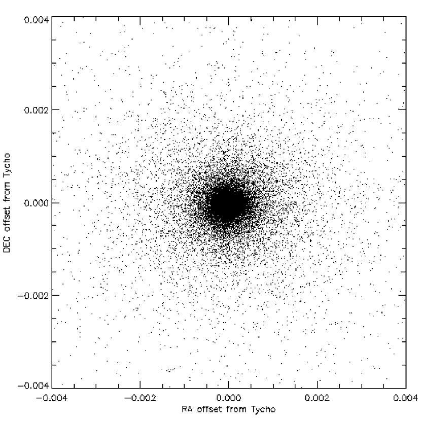
Figure 2: This figure shows astrometric residuals between Tycho and ROTSE positions for all 28740 jointly observed objects. The full size of the plot is $\pm$1 ROTSE-I pixel. RMS residuals for these bright ($m_{V}<$ 11.5) stars are about 0.1 pixel.

Astrometric calibrations are accomplished by identifying ROTSE-I objects with Tycho stars through a triangle matching routine. The transformation of CCD (x,y) to (ra,dec) is accomplished through a third order polynomial warp. The resulting quality of the astrometric calibration can be tested by examining the residuals to this fit. Astrometric residuals for a typical field are shown in Figure 2. Errors for bright ($m_{V}<12.5$) stars are $\sim$1.5”, about one tenth of a pixel.

Photometric calibration is somewhat more complex. The Tycho catalog includes only B and V photometry, and ROTSE-I images are obtained with unfiltered CCDs. We use the Tycho B and V magnitudes to produce an empirically predicted m_ROTSE for each Tycho star:

$$m_{ROTSE}=m_{V}-\frac{m_{B}-m_{V}}{1.875}$$ (1)

These color-corrected magnitudes are then used compared to ROTSE-I instrumental magnitudes to set ROTSE-I zeropoints. The net effect of this procedure is to place ROTSE observations onto a V-equivalent scale, in the sense that the average Tycho star has m_ROTSE=$m_{V}$.

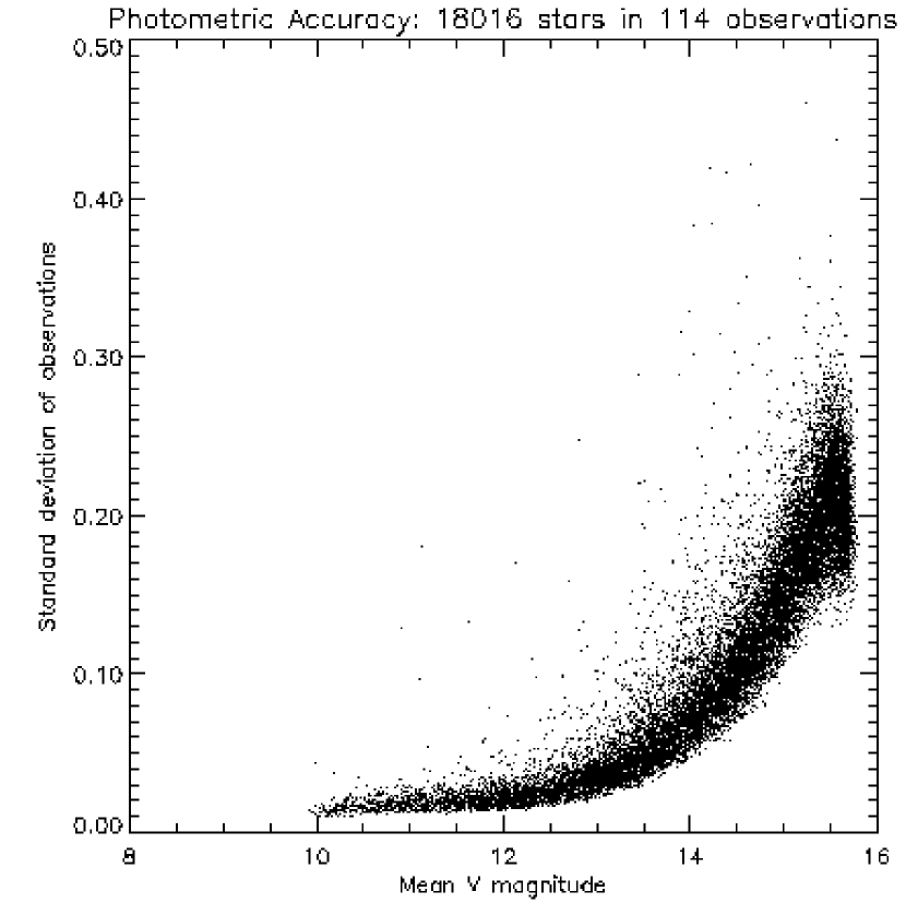
Figure 3: This figure shows photometric residuals for 114 observations of about 18,000 objects over a period of four months. Errors range from about 2% (mostly systematic) at 10th magnitude to about 20% (mostly statistical) at the magnitude limit of 15.5. Outliers are real variables.

While m_ROTSE is clearly not a standard V magnitude, this technique provides very good, stable, zeropoints. As a measure of the quality and stability of these photometric calibrations we present in Figure 3 the standard deviation of 18016 stars observed in 114 different epochs over a period of four months. The rms errors rise from $\sim$2% at 10th magnitude to about 20% at the 5$\sigma$ threshold around $m_{ROTSE}$ =15.5. These errors are typical of the fields included in this study.

The presence of many Tycho stars in each image provides an excellent opportunity for monitoring data quality. The calibration routines generate summary outputs including both astrometric and photometric fit residuals. This summary information is carefully examined before observations from a particular day are accepted and incorporated into the overall light curve catalog.

Once calibrated object lists from each observation of each field are generated, they must be collated into tables of light curves. This is done using the calibrated object positions. A requirement is imposed that each object must appear in both observations of a ROTSE pair to be included in the light curve measurement. This provides a strong veto against cosmic rays, satellite glints, etc. The output of this process is an array of light curves for each field. These light curve tables then form the input to the subsequent process of variable identification and classification.

4 Variable Identification

To automatically detect variables we implement the technique of Welch & Stetson (1993) (the WS technique) as modified by Stetson (1996). This method increases our sensitivity to periodic variables by taking advantage of paired observations. Both observations in a ROTSE-I pair are taken within 2.5 minutes. Since this time is much shorter than the period of the variables we seek, we expect the two observations to record essentially the same magnitude. For variable objects, the residuals from the comparison of each magnitude to the mean magnitude will be correlated. For stable objects there is no correlation of residuals. Products of these residuals will, for variables, generally be positive, while products of uncorrelated residuals may be either positive or negative. As a result, the sum of these products for paired observations will increase monotonically for periodic variables and cluster around zero for stable objects.

For each object with a light curve we calculate a variability index through a series of steps. The variations from the most obvious implementation of the WS technique are all designed to make the measurement more robust against the presence of a few bad observations. We begin by forming the appropriately weighted products of residuals for each pair of observations.

$$\delta_{1i}=\frac{V_{1i}-\overline{V}}{(\sigma_{V})_{1i}}$$

$$P_{i}=\delta_{1i}\delta_{2i}$$ (2)

where $\delta_{1i}$ is the uncertainty weighted residual between the first of a pair of observations of an object and the mean magnitude of that object through all observations. $P_{i}$ is the product of the residuals from a pair of adjacent observations. The mean magnitude used in this calculation is based on the robust mean of Stetson (1987). It is an iteratively weighted mean, where the weights are based on the residuals between each observation and the previously determined mean. The uncertainty $\sigma_{V}$ used for this calculation is the photometric error calculated by SExtractor added in quadrature to an assumed 2% systematic error. We generate sums of these products of residuals to calculate the variability index

$$J_{ROTSE}=\sqrt{\frac{1}{n(n-1)}}\sum_{i=1}^{n}sgn(P_{i})\sqrt{\mid P_{i}\mid}$$ (3)

where n is the number of available epochs. This varies by field from 22 to 114, primarily because different time periods were analysed for each field. This form is simpler than that discussed by Stetson (1996) because all ROTSE observations appear in pairs, and all pairs are equally weighted. As a last addition, we modify this index by the kurtosis measure of Stetson (1996). This parameter is designed to account for the fact that many real variables have sinusoidal light curves. Magnitude measures for a sinusoidal variable cluster around the maximum and minimum values. Those for a stable star with Gaussian errors cluster around the mean value. As a measure of this we calculate

$$K_{ROTSE}=\frac{\frac{1}{N}\sum_{i=1}^{N}{\mid\delta_{i}\mid}}{\sqrt{\frac{1}{N}\sum_{i=1}^{N}{\delta_{i}^{2}}}}$$

In this equation N represents the total number of observations (twice the number of epochs) and $\delta_{i}$ is the residual from the mean of each observation. This parameter has values K=1.0 for a square wave, K=0.90 for a sinusoid, and K=0.798 for a stable object with Gaussian errors. When the residuals $\delta_{i}$ are dominated by a single bad measurement with residual $\Delta$, this parameter becomes

$$K_{ROTSE}\simeq\frac{\frac{\mid\Delta\mid}{N}}{\sqrt{\frac{\Delta^{2}}{N}}}$$

$$\simeq\frac{1}{\sqrt{N}}$$ (4)

Since this goes to zero in the limit of large N, the kurtosis index helps to reduce the sensitivity to single bad observations. It also reduces our sensitivity to variables with a low duty cycle, such as flare stars and detached eclipsing binaries. We combine this with the variability index $J_{ROTSE}$ to determine the final selection index

$$I_{var}=J_{ROTSE}K_{ROTSE}/0.798$$ (5)

This is equal to J when the residuals are Gaussian, slightly amplified for sinusoidal light curves, and significantly reduced when a single bad measurement dominates the variability index J.

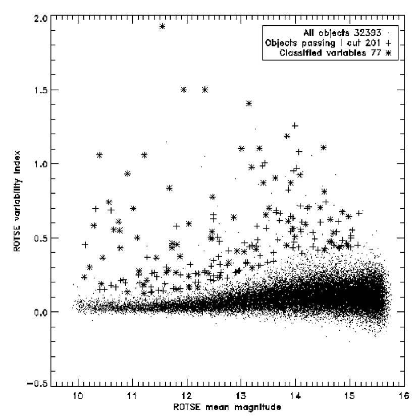
Figure 4: The ROTSE variability index $I_{var}$ calculated as described in the text is shown as a function of mean magnitude. Objects which pass the cut are shown as plus signs. Those finally selected as variable are stars. The points with large values of the variability index which are not selected have been rejected by the flare and deblending cuts described in the text.

Variable candidates are selected by examining I_var for all objects which are present in at least 11 epochs. This requirement is made because phasing is ambiguous for objects observed in fewer epochs. Figure 4 shows the distribution of I_var vs. $m_{ROTSE}$ for a typical field. For this analysis variables are selected to be those which have an I_var value more than 4.75 $\sigma$ above the mean value. In a typical camera (64 square degrees), this cut identifies between 40 and 100 candidate variables.

Two remaining cuts are made to clean the sample. Despite the robustness of I_var against objects whose light curves have just a few deviant pairs, there remain a small number of ‘flaring’ objects per field which pass our I_var cut. Some of these objects are real variables such as detached eclipsing binaries and flare stars. Since we have little information on their variability, we opt to remove them from this analysis and reserve them for further study. Such ‘flare’ objects are defined as objects for which there are at most two pairs of observations falling in the magnitude range from 0.5 to 1.0 times the absolute value of the maximum residual. This cut removes about 25% of candidate variables.

Finally, we make a cut designed to remove problems with deblending. The SExtractor deblending algorithm works well for these stellar images, but there are some cases where stars are sufficiently close to one another that they are sometimes deblended, and sometimes blended. This creates a very characteristic light curve in which the measured magnitude shifts between two distinct values. To detect these automatically, we first generate a list of ROTSE observed stars (if there are any) within a few pixels of each variable. We then extract a subset of the observations in which the candidate variable is found and its close neighbor is not. These are candidate ‘blend’ measurements. We compare the mean and standard deviation of the ‘blend’ and ‘non-blend’ measurements. If the means are separated by more than two standard deviations, the object is considered a deblending problem and removed from the variable list. The effect of this cut is strongly dependent on crowding (and hence on galactic latitude). It removes between 5% and 30% of candidate variable objects.

The output of this process is a set of objects which show moderate evidence for variability. At this point we allow the inclusion of some false variables, as we wish to maintain sensitivity to real variables of the lowest possible amplitudes. We use robust evidence of periodicity as our final restriction. This list of variable candidates includes 7396 objects, drawn from a total of 917,266 which pass the 11 epoch cut.

5 Variable Confirmation and Classification

Variable classification proceeds in two steps. First, an attempt is made to fit each light curve to a third order polynomial over the full period of observation. Since these observations cover about 100 days, this fit can be quite good for a variety of long period variables, and is used to flag long period objects. For these objects the polynomial fit parameters are used to derive an amplitude (maximum variation within the observation window) and a measure of goodness of fit. Of the 7396 variable candidates, 739 are identified as long period variables by this technique.

The second step is to attempt phasing of all objects which pass the I_var cut. For this purpose we use a cubic spline method described in detail in Akerlof, et al. (1994). This technique provides best fit periods, period error estimates, and spline fit approximations for object light curves. The general quality of these spline fits is illustrated in the sample light curves described below. In total 1195 of our 7396 variable candidates are successfully phased. The remainder (5462) are mostly near the detection threshold. Additional ROTSE data will be required to determine how many of the remaining candidates are real variables.

With phased light curves in hand, the classification process begins. Automatic classification is based on period and light curve shape, as quantified by the spline fit. We begin by Fourier analyzing the spline fit to the light curve:

$$\Delta_{m}(t)=\sum_{i=0}^{255}p_{i}cos(\frac{2\pi t}{\Gamma})$$ (6)

Where $\Delta_{m}(t)$ is the phased light curve. Classification then relies on the derived period $\Gamma$, ratios of the Fourier coefficients:

$\begin{array}[]{c}r_{1}=\frac{p_{2}}{p_{1}}\\ r_{2}=\frac{p_{3}}{p_{1}}\\ r_{3}=\frac{p_{2}}{p_{3}}\end{array}$

and the sign of the largest deviation from the mean. Cuts based on these Fourier power ratios are referred to below as ‘ratio cuts’. In addition, most classifications require that the largest power in the Fourier series is in the first term. This implies that the phased light curve has one cycle per period. The cuts used here were selected through examination of the parameters of a subset of manually classified objects. We expect them to evolve in future ROTSE variable studies.

Classification for the purposes of this study is confined to 8 classes: RRab, RRc, Delta Scuti, Cepheid, Contact Binaries, Eclipsing, Mira, and long period variable. The classifications given here should be considered preliminary. We are aware that there is not necessarily complete correspondence between our classifications and more traditional definitions of these classes. We refer to our classes as RRAB, RRC, DS, C, E, EW, M, and LPV in what follows.

RRAB stars were the original target of this project. Although most RRABs have periods from 0.3-0.9 days, some have been detected with periods as long as 2 days. Therefore the period range is defined as 0.3-2.0 d. Classification within this range is based on ratio cuts. RRAB stars are characterized by asymmetric light curves with a rapid rise followed by a slower decay. As a result we search for light curves which are not sinusoidal, but have substantial contributions from higher harmonics. RRAB stars are selected to have:

$\begin{array}[]{ccc}0.08<r_{1}<1.0,&0.01<r_{2}<1.0,&r_{3}>0.6\end{array}$

The RRC, DS, and C types are quite similar in the sense that all have more or less sinusoidal light curves. The primary distinction between these classes is period range. We begin by requiring that the contribution from higher harmonics be small. All three classes share the same ratio cuts:

$\begin{array}[]{cc}r_{1}<0.16,&r_{2}<0.024\end{array}$

Those phased objects which pass these cuts we classify as DS ($\Gamma<0.2$d), RRC ($0.2$d$<\Gamma<1.0$d), or C ($1.0$d$<\Gamma<50.0$d).

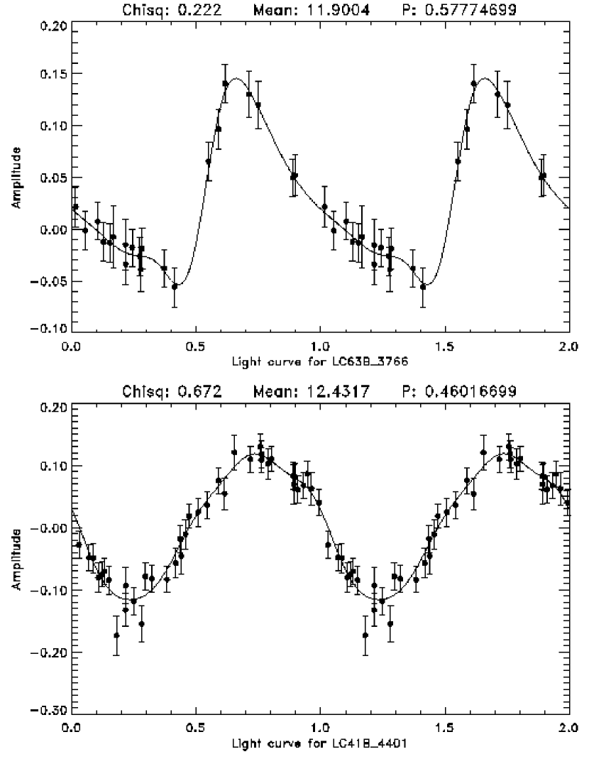
Figure 5: Light curves for an example RRAB (top) and RRC (bottom) in the overlap region of period and amplitude space. The RRAB exhibits a steep rise compared to the nearly sinusoidal RRC light curve shape.

This RRC classification overlaps with the low end of the RRAB period and ratio space. This is not an enormous problem, as the majority of RRC stars have periods less than 0.4 d. To accommodate the region of overlap we tighten the RRC ratio cuts to $r_{1}<0.08$ and $r_{2}<0.01$ for the range $\Gamma>0.4$ when the amplitude $>$ 0.35 m. This accounts for the only apparent difference between RRAB and RRC objects in this range; the RRC stars have lower amplitude and a light curve too sinusoidal to be called RRAB. A comparison of RRAB and RRC light curves in this period and amplitude range is given in Figure 5.

Eclipsing objects include the EW (contact) and E (detached) types. There are no period restrictions for selection of eclipsing systems. EW objects are selected as those with

$\begin{array}[]{cc}0.04<r_{1}<0.2,&0.007<r_{2}<0.04\end{array}$

Since these objects tend to overlap with RRC and DS objects, the distinguishing feature becomes the sign of the greatest deviation. For EW stars, the greatest deviation is always less than the mean. For RRC and DS stars the greatest deviation tends to be brighter than the mean. Systems which receive the E classification also require a negative greatest deviation. E type systems are treated in two sets, those with eclipses of equal depth, and those with eclipses of different depths. This second case is the only class which we allow to have two cycles per period. For those objects which have minima of equal depth, the real orbital period of the system is twice the photometric period. Periods for equal depth E and EW type systems are corrected for this effect once classification is complete.

As a final step for this classification, each light curve is checked by visual inspection, allowing for small adjustments to classification. In addition, each light curve and its classification was manually graded for quality from 10 (excellent) to 1 (marginal). Experience gained from this hand-scanning convinces us that we will be able to essentially automate classification by implementing further techniques like those described by Rucinski (1997).

6 Results

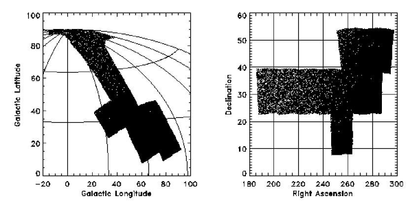
Figure 6: The locations of the nine ROTSE-I fields analyzed for this project are shown in galactic and celestial coordinates. The points represent all 77481 stars brighter than 12th magnitude seen in these fields.

In this preliminary study we have analyzed $\sim$2000 square degrees of ROTSE-I sky patrol data in an effort to assess the usefulness of these data for detection of periodic variables. The locations of these fields in galactic and celestial coordinates are shown in Figure 6. A primary conclusion of this work is confirmation that ROTSE-I data form an excellent resource for the discovery and classification of periodic variables. We have discovered a total of 1781 periodic variables, 89% of which are not included in the General Catalog of Variables Stars (Kholopov, et al., 1988) (based on position matching within a 28.8” aperture). This reiterates the long standing assertion (Paczyński, 1997) that many variable stars brighter than 15th magnitude remain to be discovered. We refer to this catalog as the ROTSE Survey for Variables 1 (RSV1).

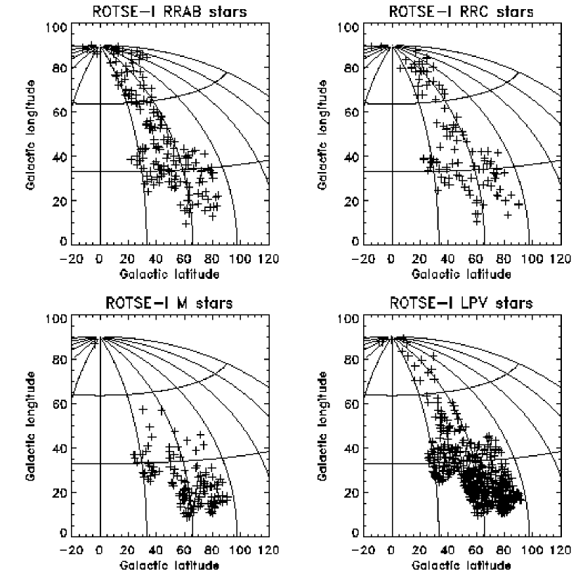
Figure 7: The distribution of ROTSE-I variables of four types in an Aitoff projection of galactic coordinates.

Some general properties of the objects discovered are presented below. Example light curves are presented for each variable class to give an idea of data quality. The distribution of several classes of objects on the sky is shown in Figure 7. The basic object list is presented in Table 1. The entire catalog, along with light curves, is available online through http://www.umich.edu/$∼$rotse.

Accurate determination of our variable detection efficiency is a complex exercise. Since detection efficiency is a strong function of period, amplitude, and light curve shape, it must be determined seperately for each variable class. This can be done correctly only after a complete understanding of the period, amplitude, and light curve shape distributions in the observing bands is obtained. These studies will be reported for each variable class in future publications.

For the moment we make a simple estimate of detection efficiency by measuring the fraction of GCVS stars recovered here. For this purpose we have selected GCVS stars within our survey area with maxima less than $m_{V}$=10 and minima greater than $m_{V}$=13. Within this sample we recover more than 80% of the RR Lyrae and Delta Scuti stars. Our efficiency for eclipsing types, as expected, varies strongly with type, from $\sim$70% for close binaries to $\sim$30% for detached systems. All 52 known Miras within the ROTSE-I magnitude range are recovered. Our lowest recovery rates are for GCVS types L and SR (the slow irregulars and semiregulars) at about 37%. This low efficiency is due to a combination of variability timescale, amplitude, and aperiodicity.

6.1 RR Lyraes

RR Lyrae stars are extremely useful as distance indicators and tracers of the structure of the Milky Way. They are attractively easy to identify and measure well. As a result they were the original target of this investigation. With a typical $M_{V}$=0.74 (Fernley, et al., 1998), RR Lyraes are detectable by ROTSE-I from 0.7 to about 7 kpc. Among all the variable types which we classify, our classification of objects as RR Lyrae stars is most secure.

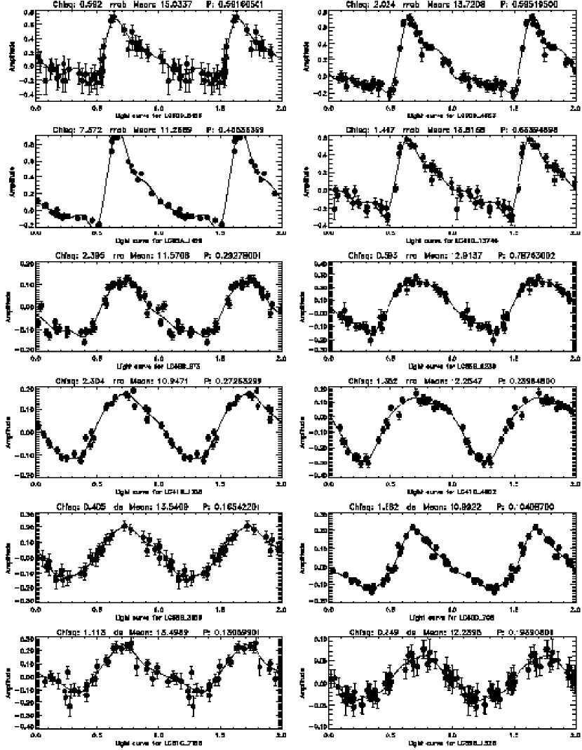
Figure 9: Example phased light curves for a random sample of ROTSE RRAB stars (top four), ROTSE RRC stars (middle four), and ROTSE DS stars (bottom four). Included above each plot are periods and mean magnitudes.

In this preliminary survey, we identify 186 RRAB stars, 126 of which are newly discovered. As these stars have large amplitude and distinctive variability, it is not surprising that a relatively large fraction (32%) are previously known. The period and amplitude distributions for these stars are shown in Figure 8. All ROTSE RRABs which appear in the GCVS are classified there as either RRAB (55 of 60) or RR (5 of 60). Sample light curves for RRAB stars are shown in Figure 9.

Since the RRAB sample has a large overlap with the GCVS, we have made direct comparisons of ROTSE and GCVS derived periods for these objects. The dependence of this period difference on $m_{ROTSE}$ is shown in Figure 10. There are 57 overlapping stars with measured GCVS periods. For two of these ROTSE measures periods substantially different from the GCVS period. In one case the ROTSE period provides an enormously better fit to the ROTSE data, suggesting that either the GCVS period is in error or the period of this object has changed. In the second the ROTSE phase coverage is incomplete. Examination of additional ROTSE data for this object shows much better agreement with the GCVS period. For the remaining 55 overlap stars the RMS period error between ROTSE and the GCVS is 0.00026 d. Typical period errors for ROTSE determinations are 0.00012 d, so these offsets are probably dominated by GCVS period errors.

In addition, we identify a total of 113 RRC stars, 104 of which are newly identified. The large fraction of newly identified RRC stars is not surprising given their relatively small pulsation amplitudes. The classification of these stars as RRCs and not, for example, contact binaries is dependent on hand scanning of the light curves. Of the nine objects known in the GCVS, seven are classified there as RRC, two as EW. Visual examination of the light curves supports the classification as RRC in both cases of disagreement. The period and magnitude histograms for these objects are also given in Figure 8. Examples of light curves for these objects are presented in Figure 9.

RRC stars make up about 9% of GCVS RR Lyraes. It is interesting to note that the RRC fraction found here, 38%, is substantially larger. This illustrates the important advantage of ROTSE-I CCD photometry over earlier wide area surveys based on photographic photometry. This difference is particularly striking for variable classes like RRCs, with mean amplitudes $A_{V}$=0.3 m. The magnitude distributions for all new and previously known RR Lyrae stars of both types are shown in Figure 11.

6.2 Delta Scuti Stars

The Delta Scuti stars are observationally (and physically) similar to the RRc class. They obey a period luminosity relation which is now well determined by Hipparcos calibration (McNamara, 1997). Their periods range from 0.1 d to 0.28 d and their amplitudes range from 0.1 to 0.5 m. We have classified 91 objects as DS stars, of which two are known from the GCVS. As with the RRC stars, the precision of ROTSE CCD photometry helps to reveal large numbers of previously undetected stars in this class. Examples of DS light curves are included in Figure 9.

6.3 Close Binary Systems

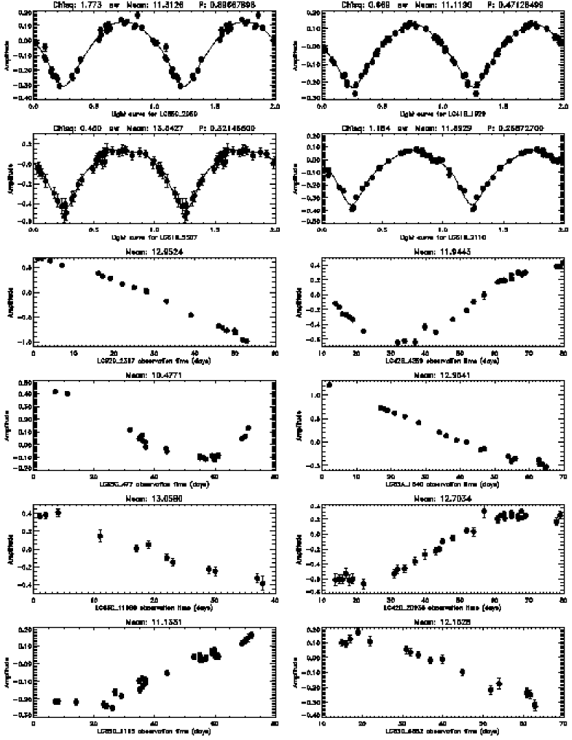
Figure 12: Example phased light curves for a random sample of ROTSE EW stars (top four), along with unphased light curves for ROTSE M stars (middle four) and ROTSE LPVs (bottom four). Included above each plot are periods (when phased) and mean magnitudes.

Close binary systems (mostly of the W UMa type) are very common in the ROTSE-I data. These objects have recently been shown to obey a reasonably tight period-color-luminosity relation (Rucinski & Duerbeck, 1997). We have identified 382 candidate close binaries, of which 368 are new. The detection of such a large number of systems is not unexpected. Most contact systems contain relatively low-mass G and K type stars. It is estimated that as many as 1 in 500 G and K type stars are members of contact binary systems. Relatively shallow, wide area surveys such as this are especially sensitive to such low luminosity objects. Examples of EW systems are presented in Figure 12.

6.4 Other Eclipsing Systems

With between 22 and 114 epochs per location this analysis has relatively poor sensitivity to widely separated eclipsing systems. Nonetheless, we identify a total of 109 eclipsing systems, 95 of which are new. This is a relatively inhomogeneous set, which includes both $\beta$ Lyrae systems and detached Algol type eclipsing binaries.

6.5 Intermediate period pulsators

We have identified 201 systems with periods from 1 d to 100 d with more or less sinusoidal light curves. All these objects are placed in class C. They are not yet fully identified, though it is clear that some are Cepheids, W Virginis stars, and RS CVn systems. Only 2 of these 201 objects are known in the GCVS; the dwarf nova AH Her, and HZ Her, a low-mass x-ray binary. An important application of the ROTSE all-sky variable survey will be identification of a complete sample of bright Cepheids for calibration of the distance ladder.

6.6 Miras and Other Long Period Variables

The long period objects in our sample are drawn from at least two different groups, Miras and red supergiant variables (RSVs). We have classified those with observed variations larger than one magnitude as M. There are 146 such objects in our sample, 66 of which are in the GCVS. Of the overlap objects, most (60 out of 66) are classified by GCVS as Miras. The remainder are classified as long period or semi-regular variables. While periods for these very long period variables cannot be firmly established by these data, we note that analysis of the full two year ROTSE-I database will be extremely effective in this regard.

Miras are among the most venerable distance indicators, and obey a good period-luminosity relation, at least in K band (Bedding & Zulstra, 1998). For Miras this PL relation is contaminated in the optical by strong TiO absorption. Pierce, Jurcevic, & Crabtree (1999) have recently shown that there is a good optical PL relation for the red supergiant variables, and it is likely that many of the objects classified here as M are actually in this class. Separation of these two classes should be possible using IR data of the type which the 2MASS survey (Beichman, 1998) will provide. As both types of stars are intrinsically very luminous ($-4<M_{ROTSE}<-7$) they can be observed in ROTSE-I data to great distance. The most luminous of these objects can be observed to about 300 kpc. While identification and period measurement of these objects can be accomplished with existing ROTSE-I data, their use as distance probes may require data in standard passbands.

We group all other long period variables into a single catch-all class. There are 534 such objects detected, of which 501 are newly discovered. This large number of new objects is remarkable, especially in light of our relatively low detection efficiency ($\sim$37%) for these objects. The combination suggests that longer duration observations will unveil substantially larger numbers of LPVs. Again, it is impossible within these four months of data to accurately determine periods for these objects. Examples of M and LPV stars are presented in Figure 12.

7 Multiwavelength Correlations

We have correlated our variable catalog with several all-sky catalogs in other wavebands. Comparison to the ROSAT All Sky Survey Bright Source Catalog (Voges, et al., 1999) yields 26 matches within a radius of 40”. Of these, only four are listed in SIMBAD; AM Her (a CV), HZ Her (an LMXRB), PW HER (an RS CVn star) and TW CrB. The last is unidentified in SIMBAD, but is clearly an EW object in ROTSE data. Of the remainder, 5 are short period eclipsing systems, one exhibits a long ($>$100 d) fade and 16 are longer period C type variables. These last may be RS CVn stars, CVs, or x-ray binaries. We are planning a program of followup spectroscopy to determine the nature of these interesting objects.

We have also cross-correlated our catalog of variables with the IRAS Point Source Catalog (Beichman, et al., 1988). A total of 269 matches are found within a radius of 40” (which is a typical IRAS error ellipse major axis). Only 85 of these are known in the GCVS. Every one of these objects is a long period variable, which we have classified as M (105), LPV (156), or C (8). All of these objects are detected in the IRAS 12 $\mu$m channel, and about half are detected in the 25 $\mu$m channel. These characteristics are perfectly consistent with their classification as pulsating giant stars.

8 Conclusions and Future Prospects

We have searched a small fraction of ROTSE-I sky patrol data for periodic variables using a robust selection technique. All detected variables have been phased and automatically classified, and the derived classifications have each been checked by visual inspection of the phased light curves. A large number of new variable stars are uncovered, including representatives of many known classes of periodic variables.

The most important conclusion of this work is confirmation that many new variables of all types await discovery at bright magnitudes, and that the ROTSE-I data are a highly effective discovery archive. These data allow accurate classification, period, and ephemeris determination for all variables with amplitudes greater than $0.1\mbox{ m}$. We identify a fraction 1781/917226 $\simeq$ 0.2% of all observed objects as variable. Because it is known that the variable selection used here is biased against some variable types this is a firm lower limit on the variability fraction.

ROTSE-I all sky patrol data are already having a real impact on the study of bright variables. In the magnitude range from 10.5-12.5 the new variables presented here (973) represent a 30% increase in the total number of GCVS variables (3162) in this magnitude range. This despite the fact that they are drawn from only 5% of the celestial sphere.

We have confirmed the expectation that many variables of modest amplitude, such as RRc and Delta Scuti stars, have escaped detection in earlier all sky searches. We find that the fraction of RR Lyraes which are of the RRC type is about 38%, in contrast to the 9% suggested by the GCVS.

The data analyzed here constitute only 5.6% of the ROTSE-I sky coverage. The entire sky visible from New Mexico has already been observed for a number of epochs ranging from 150 at -30°dec to 1100 at the north celestial pole. As this study includes substantial regions at both low (b $\sim$ 10°) and high (b=90°) galactic latitude, it is reasonable to predict the number of objects we will detect in the full survey by simple extrapolation. From this extrapolation we expect to uncover a total of about 32,000 variable stars via ROTSE-I patrol analysis.

Perhaps most important, ROTSE-I variable star selection will be carried out in a completely uniform way across the full sky north of -30°dec. The entire catalog will be based on CCD photometry, obtained with a single instrument and reduced in a single, consistent way. This will make the ROTSE-I variable catalog uniquely useful for studies of the galactic distribution of variables, and for direct studies of galactic structure.

We have concentrated here on the discovery and classification of periodic variables. Several selection criteria are deliberately biased against the inclusion of flaring objects. Analysis of these data for a variety of aperiodic transients is underway, and will be reported in subsequent publications.

In addition to extending our analysis of existing data, the ROTSE program is assembling a variety of new tools for the study of astrophysical transients. In the near future we expect to begin repeating the ROTSE-I patrol scheme with modifications to allow us to obtain three color (V, R, and I) observations. A fourth channel will retain an open CCD for increased sensitivity and comparison to earlier ROTSE-I results. In the longer term, the ROTSE program is engaged in a large scale expansion designed to improve our sensitivity to GRB optical counterparts. We are constructing an array of ten 0.45m telescopes, each with a 2°x 2°  field of view and a thinned CCD camera. These telescopes will be deployed globally to a total of 6 sites, and will provide 24 hour coverage of the sky. These ROTSE-III instruments will allow us to extend the kind of variable studies presented here to at least 19th magnitude while still covering a substantial fraction of the sky.

Table 1: Example entries from the ROTSE-I catalog.

Name	Type	Ra	Dec	$m_{ROTSE}$	$\sigma_{mR}$	$\Gamma$	$\sigma_{\Gamma}$	Amp	Quality
ROTSE1 J170711.48+454926.0	rrab	256.797852	+45.823914	14.62	0.116	0.71538502	0.00042424	0.832	7
ROTSE1 J174002.18+495318.9	c	265.009125	+49.888599	10.88	0.004	38.4667625	0.95186836	0.220	1
ROTSE1 J172429.80+460801.7	m	261.124207	+46.133808	11.07	0.004	0.00000000	0.00000000	1.490	1
ROTSE1 J171630.99+433832.1	ew	259.129150	+43.642254	11.27	0.006	0.23350200	0.00003322	0.152	5

Note. — These are sample entries from the catalog described by this paper. The amplitudes reported here are derived from spline fits to the light curves. For objects with incomplete phase coverage these can be inaccurate. Updated versions of the table, including new data, will be occasionally made available at the ROTSE web site. [The complete version of this table is in the electronic edition of the Journal. The printed edition contains only a sample]

Figure 1: Locations of ROTSE-I patrol locations are shown with the galactic plane and familiar constellations overlaid. Regular patrol observations cover all available fields north of -30°dec.

Figure 8: This figure shows the period and magnitude distributions for all the discovered RRAB and RRC type stars

Figure 10: The difference between GCVS and ROTSE derived periods is shown as a function of mean magnitude for the overlap sample of 57 RRab stars.

Figure 11: Magnitude distributions for RR Lyrae stars (RRAB and RRC) which are newly discovered (solid line), and previously known (dashed line). The dotted line shows the magnitude distribution for the total sample.

References

- Akerlof, et al. (1994) Akerlof, C., et al., 1994, ApJ, 436, 787
- Akerlof, et al. (1999) Akerlof, C., et al., 1999, Nature, 398, 400
- Barthelmy, et al. (1998) Barthelmy, S., et al., 1998, http://gcn.gsfc.nasa.gov/gcn.
- Bedding & Zulstra (1998) Bedding, T., and Zulstra, A., ApJ, 506, L47
- Beichman, et al. (1988) ed. Beichman, C., et al., (Washington, DC: GPO), NASA RP-1190.
- Bertin & Arnouts (1996) Bertin, E., and Arnouts, S., 1996, A&AS, 117, 393
- Beichman (1998) Beichman, C.A., et al., 1998, PASP, 110, 480
- Feast, et al. (1980) Feast, M.W., Catchpole, R.M., Carter, B.S., and Roberts, G., 1980, MNRAS, 193, 337.
- Fernley, et al. (1998) Fernley, J., et al., 1998, A&A, 330, 515
- Hog (1998) Hog, E., et al., 1998, A&A, 104, 340
- Kehoe, et al. (1999) Kehoe, R., et al., Proceedings of the 1999 STSCI May Symposium, astro-ph 9909219
- Kholopov, et al. (1988) Kholopov, P.N., et al., 1988, General Catalog of Variable Stars, 4th Edition (Moscow: Nauka Publishing House)
- McNamara (1997) McNamara, D.H., 1997, PASP, 109, 1221
- Paczyński (1997) Paczyński, B., 1997, in “Variable Stars and the Astrophysical Returns of Microlensing Surveys”, (Cedex, France: Editions Frontieres)
- Pierce, Jurcevic, & Crabtree (1999) Pierce, M., Jurcevic, J., and Crabtree, D., in preparation
- Rucinski (1997) Rucinski, S., 1997, AJ, 113,407
- Rucinski & Duerbeck (1997) Rucinski, S., and Duerbeck, H., 1997, PASP, 109, 1340
- Stetson (1996) Stetson, P., 1996, PASP, 108, 851
- Stetson (1987) Stetson, P., 1987, PASP, 99, 191
- Voges, et al. (1999) Voges, W., et al., 1999, A&A, 349, 389
- Welch & Stetson (1993) Welch, D., and Stetson, P., 1993, AJ, 105, 1813