Do wavelets really detect non-Gaussianity in the 4-year COBE data?

Abstract

We investigate the detection of non-Gaussianity in the 4-year COBE data reported by Pando, Valls-Gabaud & Fang (1998), using a technique based on the discrete wavelet transform. Their analysis was performed on the two DMR faces centred on the North and South Galactic poles respectively, using the Daubechies 4 wavelet basis. We show that these results depend critically on the orientation of the data, and so should be treated with caution. For two distinct orientations of the data, we calculate unbiased estimates of the skewness, kurtosis and scale-scale correlation of the corresponding wavelet coefficients in all of the available scale domains of the transform. We obtain several detections of non-Gaussianity in the DMR-DSMB map at greater than the 99 per cent confidence level, but most of these occur on pixel-pixel scales and are therefore not cosmological in origin. Indeed, after removing all multipoles beyond $\ell=40$ from the COBE maps, only one robust detection remains. Moreover, using Monte-Carlo simulations, we find that the probability of obtaining such a detection by chance is 0.59. We repeat the analysis for the 53+90 GHz coadded COBE map. In this case, after removing $\ell>40$ multipoles, two non-Gaussian detections at the 99 per cent level remain. Nevertheless, again using Monte-Carlo simulations, we find that the probability of obtaining two such detections by chance is 0.28. Thus, we conclude the wavelet technique does not yield strong evidence for non-Gaussianity of cosmological origin in the 4-year COBE data.

1 Introduction

Observations of temperature fluctuations in the cosmic microwave background (CMB) provide a valuable means of distinguishing between two competing theories for the formation of structure in the early Universe. Currently, the most favoured theory is the simple inflationary cold-dark-matter (CDM) model, for which the distribution of temperature fluctuations in the CMB should be Gaussian. The second class of theories invokes the formation of topological defects such as cosmic strings, monopoles or textures, which should imprint some non-Gaussian features in the CMB (Bouchet, Bennett & Stebbins 1988; Turok 1996). Thus, the detection (or otherwise) of a non-Gaussian signal in the CMB is an important means of discriminating between these two classes of theory.

In order to test for large-scale non-Gaussianity in the CMB, the 4-year COBE-DMR dataset (in various forms) has already been analysed using a number of different statistical techniques, as discussed below. These tests have been performed either on some combination of the 31-, 53- and 90-GHz A & B 4-year DMR maps, or the 4-year DMR maps from which Galactic emission has been removed. Two such Galaxy-removed maps are generally available, each one created using a different separation method. The DMR-DCMB map is a linear combination of all six individual COBE-DMR maps designed to cancel the free-free emission (Bennett et al. 1992), whereas the DMR-DSMB map is constructed by first subtracting templates of synchrotron and dust emission and then removing free-free emission (Bennett et al. 1994).

The first investigation of non-Gaussianity in the 4-year COBE data was performed by Kogut et al. (1996). This analysis used the 4-year DMR 53 GHz $(A+B)/2$ map at high latitudes ($|b|>20\degr$) with cut-outs near Ophiuchus and Orion (Bennett et al. 1996), and found that traditional statistics such as the three-point correlation function, the genus and the extrema correlation function, were completely consistent with a Gaussian CMB signal. Colley, Gott & Park (1996) also computed the genus statistic, but for the DMR-DCMB map with $|b|>30\degr$, and arrived at similar conclusions. The full set of Minkowski functionals were computed for the 4-year 53 GHz $(A+B)/2$ map (with a smoothed Galactic cut) by Schmalzing & Gorski (1998), taking proper account of the curvature of the celestial sphere. They also concluded that the CMB is consistent with a Gaussian random field on degree scales. On computing the bi-spectrum of the 4-year COBE data, Heavens (1998) also found no evidence for non-Gaussianity. Finally, Novikov, Feldman & Shandarin (1999) have calculated the partial Minkowski functionals for both the DMR-DCMB and DMR-DSMB maps and do report detections of non-Gaussianity, but the analysis was performed without making a Galactic cut and the detections most probably result from residual Galactic contamination.

Recently, however, two apparently robust detections of non-Gaussianity in the 4-year COBE data have been reported. Ferreira, Magueijo & Gorski (1998) applied a technique based on the normalised bi-spectrum to a map created by averaging the 53A, 53B, 90A and 90B 4-year COBE-DMR channels (each weighted according to the inverse of its noise variance) and then applying the extended Galactic cut of Banday et al. (1997) and Bennett et al. (1996). They concluded that Gaussianity can be rejected at the 98 per cent confidence level, with the dominant non-Gaussian signal concentrated near the multipole $\ell=16$. This non-Gaussian signal is certainly present in the COBE data, but Banday, Zaroubi & Gorski (1999) have now shown that it is not cosmological in origin and is most likely the result of an observational artefact. Nevertheless, using an extended bi-spectrum analysis, Magueijo (1999) reports a new non-Gaussian signal above the 97 per cent level, even after removing the observational artefacts discovered by Banday et al.

A second detection of non-Gaussianity was reported by Pando, Valls-Gabaud & Fang (1998) (hereinafter PVF), who applied a technique based on the discrete wavelet transform (DWT) to Face 0 and Face 5 of the QuadCube pixelisation of the DMR-DCMB and DMR-DSMB maps in Galactic coordinates (i.e. the North and South Galactic pole regions respectively). PVF computed the skewness, kurtosis and scale-scale correlation of the wavelet coefficients of DMR maps in certain domains of the wavelet transform, and compared these statistics with the corresponding probability distributions computed from 1000 realisations of simulated COBE observations of a Gaussian CMB sky. In all cases, they found that the skewness and kurtosis of the wavelet coefficients were consistent with a Gaussian CMB signal. On the other hand, the scale-scale correlation coefficients showed evidence for non-Gaussianity at the 99 per cent confidence level on scales of 11–22 degrees in Face 0 of both the DMR-DCMB and DMR-DSMB maps. Nevertheless, in both maps, Face 5 was found to be consistent with Gaussianity. We note that Bromley & Tegmark (1999) confirm the findings of both PVF and Ferreira et al. (1998).

In this paper, we also apply to the 4-year COBE data a non-Gaussianity test based on the skewness, kurtosis and scale-scale correlation of the wavelet coefficients. In the analysis presented below, however, we calculate the skewness and kurtosis statistics using unbiased estimators based on $k$-statistics (Hobson, Jones & Lasenby 1999 - hereinafter HJL), as opposed to the straightforward calculation of sample moments employed by PVF. For the scale-scale correlation, we adopt the same definition as that used by PVF. We also note that the analysis presented below is slightly more general than that presented by PVF, since we calculate the statistics of the wavelet coefficients in all the available domains of the wavelet transform, as opposed to using only those regions that represent structure in the maps on the same scale in the horizontal and vertical directions.

Perhaps the most important point addressed in the analysis presented here, however, is the fact that non-Gaussianity tests based on any orthogonal compactly-supported wavelet decomposition are sensitive to the orientation of the input map. This is discussed in detail below. As an illustration of this point, we therefore present the results of two separate analyses, in which the relative orientations of the input maps differ by 180 degrees. Nevertheless, it should be remembered that, in general, different techniques for detecting non-Gaussianity are each sensitive to different ways in which the data may be non-Gaussian. We should therefore not be too surprised if the detailed results of an analysis are orientation dependent. Obviously, it would be troubling if the general conclusions concerning non-Gaussianity of the data depended on orientation, but that is not the case here.

2 The wavelet decomposition

The basics of the wavelet non-Gaussianity test are discussed in detail in HJL and also by PVF and so we give only a brief outline here. The two-dimensional discrete wavelet transform (DWT) (Daubechies 1992, Press et al. 1994) performs the decomposition of a planar digitised image of size $2^{J_{1}}\times 2^{J_{2}}$ into the sum of a set of two-dimensional planar (digitised) wavelet basis functions

$$\frac{\Delta T}{T}(\mn@boldsymbol{x}_{i})=\sum_{j_{1}=0}^{J_{1}-1}\sum_{j_{2}=0}^{J_{2}-1}\sum_{l_{1}=0}^{2^{j_{1}}-1}\sum_{l_{2}=0}^{2^{j_{2}}-1}b_{j_{1},j_{2};l_{1},l_{2}}\psi_{j_{1},j_{2};l_{1},l_{2}}(\mn@boldsymbol{x}_{i}).$$ (1)

In equation (1), the wavelets $\psi_{j_{1},j_{2};l_{1},l_{2}}(\mn@boldsymbol{x})$ (with $j_{1},j_{2},l_{1},l_{2}$ taking the values indicated in the summations) form a complete and orthogonal set of basis functions. Each two-dimensional wavelet is simply the direct tensor product of the corresponding one-dimensional wavelets $\psi_{j_{1};l_{1}}(x)$ and $\psi_{j_{2};l_{2}}(y)$, which in turn are defined in terms of the dilations and translations of some mother wavelet $\psi(x)$ via

$$\psi_{j_{1};l_{1}}(x)=\left(\frac{2^{j_{1}}}{L}\right)^{1/2}\psi(2^{j_{1}}x/L-l_{1}),$$ (2)

where $0\leqslant x\leqslant L$, and a similar expression holds for $\psi_{j_{2};l_{2}}(y)$. Thus, the scale indices $j_{1}$ and $j_{2}$ correspond to the scales $L/2^{j_{1}}$ and $L/2^{j_{2}}$ in the $x$- and $y$-directions respectively (so $J_{1}$ and $J_{2}$ are the smallest possible scales – i.e. one pixel – in each direction), whereas the location indices $l_{1}$ and $l_{2}$ correspond to the $(x,y)$-position $(Ll_{1}/2^{j_{1}},Ll_{2}/2^{j_{2}})$ in the image. Since each wavelet basis function $\psi_{j_{1},j_{2};l_{1},l_{2}}(x,y)$ is localised at the relevant scale/position, the corresponding wavelet coefficient $b_{j_{1},j_{2};l_{1},l_{2}}$ measures the amount of signal in the image at this scale and position.

2.1 Orientation sensitivity

At this point, it is important to note the sensitivity of the orthogonal wavelet decomposition to the orientation of the original input map. As shown by Daubechies (1992), it is impossible to construct an orthogonal wavelet basis, in which the basis functions are both symmetric (or anti-symmetric) and have compact support. This asymmetry of the basis functions is the cause of the orientation sensitivity. This is most easily appreciated by considering an input map consisting of just one of the wavelet basis functions. If this map is rotated through 180 degrees (say), then because the basis functions are asymmetric it is not possible to represent the rotated basis functions in terms of just one of the original basis function. Instead, the signal in the rotated map must be represented by several wavelet basis functions with different scale and position indices. Thus any statistics based on the wavelet coefficients are sensitive to the orientation of the original input map. Since the origin of this effect is the asymmetry of the one-dimensional wavelet basis functions, it also occurs for two-dimensional orthogonal wavelet decompositions based on the Mallat algorithm (Mallat 1989), which is also commonly called the multiresolution analysis method. In order to obtain wavelet statistics that are invariant under 90, 180, 270 degrees rotations of the input image (and also insensitive to cyclic translations of the image by an arbitrary number of pixels in each direction), it is necessary to use the à trous wavelet algorithm (see e.g. Starck, Murtagh & Bijaoui 1998) with a symmetric filter function. The application of this technique to the detection of non-Gaussianity in the CMB will be presented in a forthcoming paper.

Figure 1: The regions of the two-dimensional wavelet domain for a $32\times 32$ image. The italic numbers show the value of $k=2^{j_{1}}+2^{j_{2}}$ in each region; see text for details.

2.2 Application to COBE data

In this paper, we will be concerned with Face 0 and Face 5 of the COBE QuadCube pixelisation scheme in Galactic coordinates, each of which consists of $32\times 32$ equal-area pixels (i.e. $J_{1}=J_{2}=5$) of size $(2.8\degr)^{2}$. Thus the scale $j$ corresponds to an angular scale of $2.8\times 2^{4-j}$. Following the discussion by HJL, the structure of the corresponding wavelet domain is shown in Fig. 1, where the pixel numbers are plotted on a logarithmic scale. We see that the domain is partitioned into separate regions according to the scale indices $j_{1}$ and $j_{2}$ in the horizontal and vertical directions respectively. Thus regions with $j_{1}=j_{2}$ contain wavelets basis functions that represent the image at the same scale in the two directions, whereas regions with $j_{1}\neq j_{2}$ describe the image on different scales in the two directions. As discussed in HJL, regions with $j_{1}=0$ or $j_{2}=0$ actually contain basis functions that are tensor products of different one-dimensional basis and so for the remainder of this paper we restrict our attention to regions with $j_{1},j_{2}\geqslant 1$. We also define the integer variable $k=2^{j_{1}}+2^{j_{2}}$, which serves as a measure of inverse scale length, and is constant within each region of the wavelet domain. We note that the value of $k$ is not altered if the values $j_{1}$ and $j_{2}$ are interchanged. In this paper, we also restrict ourselves to the Daubechies 4 wavelet basis used by PVF, although analogous analyses may also be performed for other orthogonal discrete wavelet bases, and indeed similar results to those presented in Section 3 are obtained.

2.3 Skewness and kurtosis spectra

Following HJL, when considering the statistics of the wavelet coefficients $b_{j_{1},j_{2};l_{1},l_{2}}$ of an image, it is useful to consider separately all those coefficients that share each value of $k$. For each value of $k$, we then use the corresponding wavelet coefficients to calculate estimators of the skewness $\hat{S}$ and (excess) kurtosis $\hat{K}$ of the parent distribution from which the coefficients were drawn. We therefore obtain the skewness and kurtosis ‘spectra’ $\hat{S}(k)$ and $\hat{K}(k)$ for the image.

As mentioned in the Introduction, at this point our method diverges from that used by PVF in two ways. Firstly, PVF only consider regions of the wavelet domain for which $j_{1}=j_{2}$ and $j_{1},j_{2}\geqslant 1$ (i.e. $k=4,8,16,32$), whereas we consider all regions with $j_{1},j_{2}\geqslant 1$. Secondly, we calculate the estimators $\hat{S}$ and $\hat{K}$ in a different way from that adopted in PVF, as follows. At each value of $k$ the skewness and (excess) kurtosis of the parent distribution of the wavelet coefficients are given by

$$S = \mu_{3}/\mu_{2}^{3/2}=\kappa_{3}/\kappa_{2}^{3/2},$$ (3)

$$K = \mu_{4}/\mu_{2}^{2}-3=\kappa_{4}/\kappa_{2}^{2},$$ (4)

where $\mu_{n}$ is the $n$th central moment of the distribution and $\kappa_{n}$ is the $n$th cumulant (see HJL for a brief discussion). In PVF, the estimators $\hat{\mu}_{n}$ of the central moments are simply taken to be the central moments of the sample of wavelet coefficients. It is easily shown, however, that these estimators are biased, so that $\langle\hat{\mu}_{n}\rangle\neq\mu_{n}$, and this bias is quite pronounced when the sample size is small (as it is in this case). PVF then estimate the skewness and (excess) kurtosis by inserting the biased estimators $\hat{\mu}_{n}$ into (3) and (4) respectively. Thus, the corresponding estimators $\hat{S}$ and $\hat{K}$ are also significantly biased. In this paper, we instead calculate our estimates of the skewness and (excess) kurtosis using $k$-statistics (see Kenney & Keeping 1954; Stuart & Ord 1994; HJL). These provide unbiased estimates $\hat{\kappa}_{n}$ of the cumulants of the parent population from which the wavelet coefficients were drawn. These unbiased estimators of the cumulants are then inserted into (3) and (4) to obtain the estimators $\hat{S}$ and $\hat{K}$.

2.4 Scale-scale correlation spectrum

In addition to the skewness and kurtosis spectra, we may also measure the correlation between the different domains of the wavelet transform by defining the estimators of the scale-scale correlation as

$$\hat{C}^{p}_{j_{1},j_{2}}=\frac{2^{j_{1}+j_{2}+2}\sum_{l_{1}}\sum_{l_{2}}b^{p}_{j_{1},j_{2};[l_{1}/2],[l_{2}/2]}b^{p}_{j_{1}+1,j_{2}+1;l_{1},l_{2}}}{\sum_{l_{1}}\sum_{l_{2}}b^{p}_{j_{1},j_{2};[l_{1}/2],[l_{2}/2]}\sum_{l_{1}}\sum_{l_{2}}b^{p}_{j_{1}+1,j_{2}+1;l_{1},l_{2}}}.$$ (5)

In equation (5), the sums on $l_{1}$ extend from $0$ to $2^{j_{1}+1}-1$ (similarly for $l_{2}$), $p$ is an even integer and $[~{}]$ denotes the integer part. Thus $C^{p}_{j_{1},j_{2}}$ measures the correlation between the wavelet coefficients in the domains $(j_{1},j_{2})$ and $(j_{1}+1,j_{2}+1)$. In PVF, it was assumed that $j_{1}=j_{2}$, so that the correlation of wavelet coefficients were only calculated between adjacent diagonal domains in Fig. 1. When $j_{1}\neq j_{2}$, however, it is convenient to extend the sums in (5) to include also the corresponding domains with $j_{1}$ and $j_{2}$ interchanged. Thus, in each case, we in fact measure the correlation between wavelet coefficients with inverse scalelengths of $k$ and $2k$ respectively (see Fig. 1). For each possible value of $k$, we denote this correlation by $\hat{\cal C}^{p}(k)$, thereby producing a scale-scale correlation spectrum. Following PVF, we restrict our analysis to the case where $p=2$.

2.5 The non-Gaussianity test

The skewness, (excess) kurtosis and scale-scale correlation spectra $\hat{S}(k)$ , $\hat{K}(k)$ and $\hat{\cal C}^{2}(k)$ of the wavelet coefficients form the basis of the non-Gaussianity test. The procedure is as follows. We first calculate the $\hat{S}(k)$, $\hat{K}(k)$ and $\hat{\cal C}^{2}(k)$ spectra for Face 0 or Face 5 of the 4-year COBE map. We then generate 5000 realisations of an all-sky CMB map drawn from an inflationary/CDM model with parameters $\Omega_{\rm m}=1$, $\Omega_{\Lambda}=0$, $h=0.5$, $n=1$ and $Q_{\rm rms-ps}=18$ $\mu$K, convolved with a $7\degr$-FWHM Gaussian beam. For each realisation, we then add random Gaussian pixel noise, where the rms of the noise in each pixel is taken from the COBE rms noise map. The $\hat{S}(k)$, $\hat{K}(k)$ and $\hat{\cal C}^{2}(k)$ spectra are then calculated for Face 0 and Face 5 of each of the 5000 realisations to obtain approximate probability distributions for the $\hat{S}(k)$, $\hat{K}(k)$ and $\hat{\cal C}^{2}(k)$ statistics when the CMB signal is the chosen Gaussian inflationary/CDM model. By comparing these probability distributions with the corresponding spectra for Face 0 and Face 5 of the COBE map, we thus obtain (at each $k$-value) an estimate of the probability that the CMB signal in the DMR-DSMB map is drawn from a Gaussian ensemble characterised by the chosen inflationary/CDM model. For each face, however, we obtain skewness and kurtosis statistics at ten different $k$-values, and six different scale-scale correlation statistics. Thus, the total number of statistics obtained for each face is 26, and care must be taken in assessing the significance of non-Gaussianity detections at individual $k$-values (see below). As discussed in section 2.1, however, the orthogonal wavelet decomposition is sensitive to the orientation of the input map. Thus, we repeat the above non-Gaussianity test for the case where Face 0 and Face 5 are both rotated through 180 degrees.

It is also clear that, to some extent, the results of such an analysis will depend on the chosen parameters in the inflationary/CDM model via the corresponding predicted ensemble-average power spectrum $C_{\ell}$, from which the 5000 realisations are generated. Nevertheless, since at each $k$-value the skewness and kurtosis statistics contain the variance $\mu_{2}$ of the wavelet coefficients in their denominators, and the scale-scale correlation in (5) is similarly normalised, we would expect these statistics to be relatively unaffected by changing the power spectrum of the inflationary/CDM model. As an interesting test, we repeated our entire analysis for the case where the 5000 realisations were instead generated using the maximum-likelihood $C_{\ell}$ spectrum calculated from the 4-year COBE data by Gorski (1997). As expected, we found that the results were virtually identical to those presented in the next Section.

3 Results

3.1 The DMR-DSMB map

In this Section, we present the results of the wavelet non-Gaussianity test when applied to Face 0 and Face 5 of the 4-year COBE DMR-DSMB map in Galactic coordinates. As mentioned in the Introduction, this Galaxy-removed map is constructed by first subtracting templates of synchrotron and dust emission and then removing the free-free emission (Bennett et al. 1994). We find that the results of the non-Gaussianity test are similar for both the DMR-DSMB and DMR-DCMB Galaxy-removed maps.

The resulting $\hat{S}(k)$, $\hat{K}(k)$ and $\hat{\cal C}^{2}(k)$ spectra for Face 0 and Face 5 of the DSMB map are plotted in Fig. 2. In each plot, the crosses correspond to the values derived from the DSMB map orientated in the same manner as that used by PVF (orientation A), the solid squares correspond to the values obtained from the DSMB map after rotating it through 180 degrees (orientation B), and the open circles denote the mean of corresponding distribution derived from the simulated COBE observations of the 5000 realisations of the inflationary/CDM model. The error bars denote the 68, 95 and 99 per cent limits of the distributions. These distributions were found to be virtually indistinguishable for the two orientations of the COBE data. For convenience, the $\hat{S}(k)$ and $\hat{K}(k)$ spectra have been normalised so that the variance of each distribution is equal to unity. Thus, for any particular $k$-value, a estimate of the significance level can be read off directly from the scale on the vertical axis.

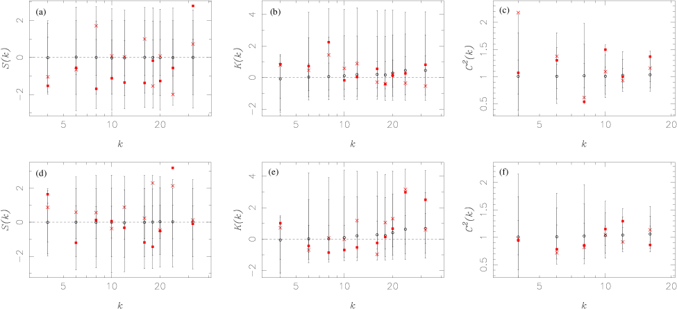
Figure 2: The $\hat{S}(k)$, $\hat{K}(k)$ and $\hat{\cal C}^{2}(k)$ spectra for Face 0 [plots (a), (b) and (c)] and Face 5 [plots (d), (e) and (f)] of the DMR-DSMB map. The crosses correspond to the orientation used by PVF (orientation A), whereas the solid squares correspond to the map rotated through 180 degrees (orientation B). The open circles show the mean value for each statistic obtained from 5000 simulated COBE observations of CDM realisations, and the error bars denote the 68, 95 and 99 per cent limits of the corresponding distribution. For convenience, the $\hat{S}(k)$ and $\hat{K}(k)$ spectra have been normalised at each value of $k$ such that the variance of the distribution obtained from the 5000 CDM realisations is equal to unity.

As mentioned above, we calculate the $\hat{S}(k)$ and $\hat{K}(k)$ spectra for all available domains of the wavelet transform, and the $\hat{\cal C}^{2}(k)$ spectrum for all pairs of domains whose $k$-values differ by a factor of 2 (with $j_{1},j_{2}\geqslant 1$ in each case; see Fig. 1). In contrast, PVF only considered domains with $j_{1}=j_{2}$ and thus only obtained $\hat{S}(k)$ and $\hat{K}(k)$ values for $k=4,8,16,32$, and $\hat{\cal C}^{2}(k)$ values at $k=4,8,16$.

We see from Fig. 2 that for orientation A (crosses), all the points in the skewness and kurtosis spectra lie comfortably within their respective Gaussian probability distributions for both faces. In the scale-scale correlation spectrum, however, we confirm PVFs finding of a point at $k=4$ that lies slightly outside the 99 per cent confidence limit. On the other hand, for orientation B (solid squares) we obtain two skewness detections someway beyond the 99 per cent confidence limit. These occur in Face 0 at $k=32$ and in Face 5 at $k=24$. From Fig. 1, however, we see that these $k$-values correspond to wavelet basis functions on small scales, corresponding to pixel-to-pixel variations in the COBE map. Thus it is unlikely that this non-Gaussianity is cosmological in origin; we return to this point below. The kurtosis spectrum and scale-scale correlation spectra show no strong non-Gaussian outliers for this orientation.

In order to investigate the robustness of the high-$k$ outliers in the $\hat{S}(k)$ spectra for orientation B, we repeated the analysis for the DSMB map with all multipoles above $\ell=40$ removed. A similar filtering process was also performed on each of the 5000 CDM realisations. Since the 7-degree FWHM COBE beam essentially filters out all modes beyond $\ell=40$, we would expect these modes to contain no contribution from the sky and consist only of instrumental noise or observational artefacts. We also repeated the filtering process for orientation A. The corresponding $\hat{S}(k)$, $\hat{K}(k)$ and $\hat{\cal C}^{2}(k)$ spectra for two orientations of Face 0 and Face 5 of the filtered DSMB map are plotted in Fig. 3.

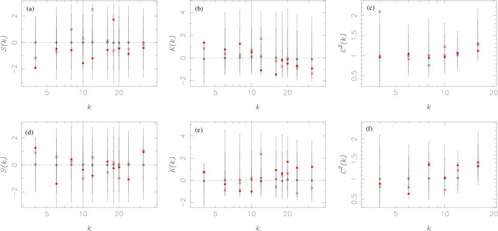
Figure 3: As in Fig. 2, but for the DMR-DSMB map with all mutlipoles above $\ell=40$ removed.

We see immediately that the high-$k$ skewness detections that were present in the unfiltered map have now disappeared. This suggests that the non-Gaussianity present in the original DSMB map is not cosmological in origin, and is most likely an artefact resulting from the algorithm used to subtract Galactic emission. From Fig. 3(c), we also note that the three points that lay outside the 95 per cent limit in the $\hat{\cal C}^{2}(k)$ spectrum for Face 0 of the original DSMB map in orientation B (see Fig. 2(c)) have all now been brought well within the Gaussian error bars. Thus we find no strong evidence for non-Gaussianity in the filtered DSMB map in orientation B. For orientation A, however, as we might expect, the level of significance of the $\hat{\cal C}^{2}$ detection at $k=4$ was only slightly reduced by the filtering process.

3.2 The 53+90 GHz coadded map

Since the above analysis suggests some non-Gaussianity on pixel scales in the DSMB map, possibly introduced by the Galaxy subtraction algorithm, we repeat the analysis for the inverse noise variance weighted average of the 53A, 53B, 90A and 90B COBE DMR channels.

Fig. 4 shows the $\hat{S}(k)$, $\hat{K}(k)$ and $\hat{\cal C}^{2}(k)$ spectra for Face 0 and Face 5 of the $53+90$ GHz coadded map in both orientations. For orientation A (crosses), none of the skewness, kurtosis or scale-scale correlation statistics lies outside the corresponding 99 per cent limit. Also, for orientation B (solid squares), we see that, in contrast to the DSMB map, no large detections of non-Gaussianity are obtained at high $k$ in the skewness spectra. Nevertheless, outliers do occur at the 99 per cent level for Face 0 in the $\hat{K}(k)$ spectrum at $k=4$, and for Face 5 in the $\hat{\cal C}^{2}(k)$ at $k=6$ and $k=12$. Indeed, the last of these lies someway outside the 99 per cent confidence limit. However, this statistic measures the correlation between the wavelet coefficients in the domains with $k=12$ and $k=24$, and is therefore influenced primarily by features in the map on the scale of one or two pixels in size.

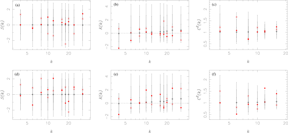
Figure 4: As in Fig. 2, but for the 53+90 GHz coadded map.

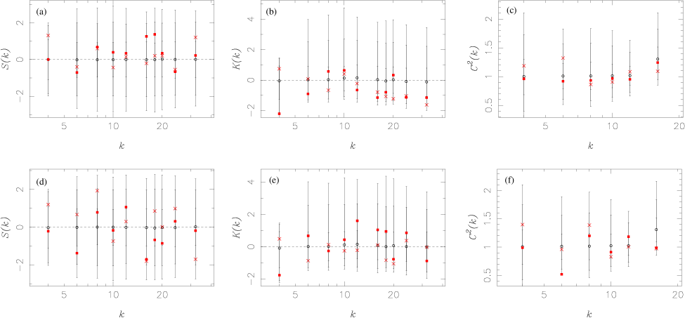
Figure 5: As in Fig. 2, but for the 53+90 GHz coadded map with all multipoles above $\ell=40$ removed.

We once again tested the robustness of these putative detections of non-Gaussianity by repeating the analysis after removing all multipoles above $\ell=40$ from the COBE map and the CDM realisations. The resulting spectra are shown in Fig. 5. From Fig. 5(f), we see that the large outlier in $\hat{\cal C}^{2}(12)$ that was obtained for the unfiltered map in orientation B has now reduced to well within the Gaussian error bars. This suggests that the noise in Face 5 of the coadded map may contain some non-Gaussian component. Nevertheless, the two outliers at the 99 per cent limit in $\hat{K}(4)$ for Face 0 and $\hat{\cal C}^{2}(6)$ for Face 5 in orientation B remain unaffected by the filtering process, and thus might be interpreted as robust signatures of non-Gaussianity on large scales.

It is, however, important to remember that, although the significance level is above the 99 per cent level for these individual statistics, we must take into account the fact that no outliers are found in the large number of other statistics we have calculated; this is discussed below. It should also be bourne in mind that no Galaxy subtraction has been performed on the 53+90 GHz coadded map. Although, our analysis is restricted to Face 0 and Face 5 of the COBE QuadCube, which lie outside the standard Galactic cut, it is possible that these faces may be contaminated to some extent by high-latitude Galactic emission.

4 Discussion and conclusions

We have presented an orthogonal wavelet analysis of the 4-year COBE data, in order to search for evidence of large-scale non-Gaussianity in the CMB. In particular, we identify an orientation sensitivity associated with this method, which must be borne in mind when assessing its results.

We find that several statistics in the $\hat{S}(k)$, $\hat{K}(k)$ and $\hat{\cal C}^{2}(k)$ spectra for the COBE DSMB and 53+90 GHz coadded maps (in orientations A and B) lay outside the 99 per cent limit of the corresponding probability distributions derived from 5000 simulated COBE observations of CDM realisations. However, only one such outlier in the DSMB map and two outliers in the 53+90 GHz coadded map were found to be robust to the removal of all multipoles above $\ell=40$ in the COBE map and CDM realisations. In the DSMB map, this occurs in $\hat{\cal C}^{2}(4)$ for Face 0 in orientation A, and in the 53+90 GHz coadded COBE map the outliers are in $\hat{K}(4)$ for Face 0 and $\hat{\cal C}^{2}(6)$ for Face 5, both in orientation B.

We must, however, take care in assessing the significance of these outliers. For each face and orientation we calculate 26 different statistics. Thus for each data set (either DSMB or 53+90 GHz coadded), the total number of statistics is $2\times 2\times 26=104$, and we must take proper account of the fact that a large number of these show no evidence of non-Gaussianity (see, for example, Bromley & Tegmark 1999). Since the statistics presented here are not independent of one another and generally do not possess Gaussian one-point functions, the only way of obtaining a meaningful estimate of the significance of our results is by Monte-Carlo simulation. Indeed, in their bi-spectrum analysis of the 4-year COBE data, Ferreira et al. (1998) used Monte-Carlo simulations and a generalised $\chi^{2}$-statistic to assess their results. In our case, we adopt a slightly different approach and simply use the 5000 CDM realisations to estimate the probability of obtaining a given number of robust outliers at $>99$ percent level in any of our 104 statistics, even when the underlying CMB signal is Gaussian. For the DSMB data, we obtained one robust outlier, and the corresponding probability of this occuring by chance was found to be 0.59. For the 53+90 GHz coadded data, two outliers were obtained, and the corresponding probability is 0.28. Therefore planar orthogonal wavelet analysis of the 4-year COBE data can only rule out Gaussianity at the 41 per cent level in the DSMB data and at the 72 per cent level in the 53+90 GHz coadded data. Thus, we conclude that this method does not provide strong evidence for non-Gaussianity in the CMB.

References

- [1] Banday A.J., Gorski K.M., Bennett C.L., Hinshaw G., Kogut A., Lineweaver C., Smoot G.F., Tenorio L., 1997, ApJ, 475, 393
- [2] Banday A.J., Zaroubi S., Gorski K.M., 2000, ApJ, in press (astro-ph/9908070)
- [3] Bennet C.L. et al., 1992, ApJ, 396, L7
- [4] Bennet C.L. et al., 1994, ApJ, 436, 423
- [5] Bennet C.L. et al., 1996, ApJ, 464, 1
- [6] Bouchet F.R., Bennett D.P., Stebbins A., 1988, Nat, 335, 410
- [7] Bromley C.L., Tegmark M., 1999, ApJ, 524, L79
- [8] Colley W.N., Gott III J.R., Park C. 1996, MNRAS, 281, L82
- [9] Daubechies I., 1992, Ten Lectures on Wavelets. S.I.A.M., Philadelphia
- [10] Ferreira P., Magueijo J., Gorski K.M., 1998, ApJ, 503, L1
- [11] Gorski K.M., 1997, in Bouchet F.R., Gispert R., Guideroni B., Tran Thanh Van J.,eds, Proc. 16th Moriond Astrophysics Meeting, Microwave Anisotropies. Editions Frontière, Gif-sur-Yvette, p. 77
- [12] Heavens A.F., 1998, MNRAS, 299, 805
- [13] Hobson M.P., Jones A.W., Lasenby A.N., 1999, MNRAS, 309, 125 (HJL)
- [14] Kenney J.F., Keeping E.S., 1954, Mathematics of Statistics (Part I). Van Nostrand, New York
- [15] Kogut A., Banday A.J., Bennett C.L., Gorski K.M., Hinshaw G., Smoot G.F., Wright E.L., 1996, ApJ, 464, L29
- [16] Magueijo J., 1999, ApJ, submitted (astro-ph/9911334)
- [17] Mallat S.G., 1989, IEEE Trans. Acoust. Speech Sig. Proc., 37, 2091
- [18] Novikov D., Feldman H.A., Shandarin S.F., 1999, Int. J. Mod. Phys. D, 8, 291
- [19] Pando J., Valls-Gabaud D., Fang L.-Z., 1998, Phys. Rev. Lett., 81, 4568 (PVF)
- [20] Press W.H., Teukolsky S.A., Vettering W.T., Flannery B.P., 1994, Numerical Recipes. Cambridge University Press, Cambridge
- [21] Schmalzing J., Gorski K.M., 1998, MNRAS, 297, 355
- [22] Starck J.-L., Murtagh F., Bijaoui A., 1998, Image Processing and Data Analysis. Cambridge University Press, Cambridge
- [23] Stuart A., Ord K.J., 1994, Kendall’s Advanced Theory of Statistics (Volume I). Edward Arnold, London
- [24] Turok N., 1996, ApJ, 473, L5