Ongoing Large Surveys for
Metal-Poor Stars in the Galactic Halo

Abstract

We report on two major surveys for metal-poor stars in the galactic halo, the HK survey, and the Hamburg/ESO survey, which have been undertaken in order to provide targets for high-resolution spectroscopy with the Subaru HDS and other large telescopes. We compare basic properties of these two surveys and their current status, and add some historical remarks.

The candidate selection procedures of both surveys are described in detail. We evaluate the candidate selection by comparing effective yields (EYs) of the survey techniques for the identification of metal-poor stars. It is found that EY for stars below [Fe/H]$=-2.0$ in the HES can be up to $\sim 80$ % for stars selected by automatic classification from machine-scanned unwidened plates, whereas in the HK survey, where stars are selected by visual inspection of widened survey plates, the EY is between 11 % and 32 %, depending on whether a pre-selection based on $BV$ photometry has been applied.

Finally, we describe techniques used for determining stellar parameters of the survey stars by means of moderate resolution follow-up spectroscopy, and additional $UBV$ photometry. While follow-up observations of HES stars have just been started, the HK survey has already produced a list of $\sim 4700$ stars with estimates of [Fe/H] typically precise to $\pm 0.2$ dex, some 1000 of which have [Fe/H] $<-2.0$, and roughly 100 of which have [Fe/H] $<-3.0$.

To appear in: Proceedings of Workshop on Subaru HDS, Tokyo, December 8.–10., 1999

1 Introduction

With the advent of several new 8 m class telescopes, e.g. Subaru, and the VLT telescopes, it is anticipated that many new insights into the nature of the Galactic halo, the chemical evolution of our Galaxy, and the first stars to have formed within it, will soon be in the offing. However, it would be impossible to obtain such exciting results if there where no large surveys that can provide targets for high-resolution, high-$S/N$ observations with these new instruments of discovery. In this article, we give a detailed comparison of two such surveys, namely the HK survey (Beers et al. 1985, 1992), and the Hamburg/ESO survey (HES; Wisotzki et al. 1996, 2000). For a comprehensive review of past, present and future surveys for metal-poor stars we refer the reader to Beers (2000a).

2 Basic properties of the surveys

In this section we compare basic properties of the HK and HE surveys, and add some historical remarks. An overview of the survey properties is given in Tab. 1.

		HK survey	HES
	north	0.6 m Burrell Schmidt	—
Telescope	south	0.6 m Curtis Schmidt	1 m ESO Schmidt
Magnitude range		$11.0\lesssim B\lesssim 15.5$	$14.0\lesssim B\lesssim 17$
Widened?		yes	no
	north	$2800\,\Box^{\circ}$	—
Area	south	$4100\,\Box^{\circ}$	$7600\,\Box^{\circ}$
Objective prism		$4^{\circ}$	$4^{\circ}$
Dispersion		$180$ Å/mm	$450$ Å/mm
Spectral resolution		$\sim 5\,$Å	$\sim 10\,$Å at Ca II K
Photographic emulsion		103a-O/IIa-O	IIIa-J
Filter?		interference/Ca H+K	no
Wavelength range		$3875\,$Å$<\lambda<4025\,$Å	$3200\,$Å$<\lambda<5200\,$Å
Candidate selection		visual inspection	automated

Table 1: Comparison of the HK survey and the Hamburg/ESO survey (HES).

2.1 HK survey

In 1978, G. Preston and S. Shectman of the Carnegie Observatories of Washington started an objective-prism survey for the discovery of numerous metal-poor and field horizontal-branch stars in the Galaxy. This was at a time when it was generally assumed that stars more metal-deficient than the most metal-poor globular clusters (${\rm[Fe/H]}\sim-2.5$) do not exist. In 1983 Beers joined the team, and later expanded the survey with an additional 240 plates in the southern and northern hemispheres. This survey, once referred to as the “Preston-Shectman Survey,” is now widely known as the “HK survey.” This is because in addition to a 4$\arcdeg$ objective prism (leading to a seeing-limited spectral resolution of $\sim 5$ Å), an interference filter was mounted on the plate holder to limit the wavelength coverage to $\sim 150\,$Å centered on the Ca II H+K resonance lines, effectively reducing the sky background level so that long exposures (typically 90 minutes) could be obtained. By 1992, 308 acceptable-quality plates were obtained (275 of which are unique) with the 60 cm Burrell Schmidt (northern hemisphere) and Curtis Schmidt (southern hemisphere) telescopes, each plate covering $5\arcdeg\times 5\arcdeg$ of the sky. Further extension of the survey area was prevented by the shortage of photographic plates with 103a-O and IIa-O emulsions.

2.2 HES

The HES was started in 1989 as an ESO Key Programme (P.I.: D. Reimers; Project Manager: L. Wisotzki). Its main aim is to find bright quasars. However, it was recognized right at the start that with the HES’ seeing-limited spectral resolution of $\sim 15$ Å at H$\gamma$, it would be feasible to do a lot of interesting stellar work as well. In 1994, Christlieb joined the HES group, and began development of methods for the systematic exploitation of the stellar content of the HES. By that time almost half of the objective-prism plates had already been taken in service mode, with the ESO 1 m-Schmidt telescope and its $4\arcdeg$ prism, and most of the data reduction software had been developed by L. Wisotzki and T. Köhler. Because the HES plates were taken without a filter, resulting in a wavelength coverage of $3200\,\mbox{{\AA}}<\lambda<5200\,\mbox{{\AA}}$, some care had to be taken with the identification of overlapping spectra. Moreover, since the HES was primarily a quasar survey, it was deemed not useful to work in fields with too high foreground extinction. As a result, the main criteria defining the HES survey area are the mean star density, $\rho$, and column density of neutral hydrogen, N${}_{\mbox{\scriptsize H}}$:

$$\rho < 100\mbox{ stars}/\mbox{deg}^{2}$$

$$\mbox{N}_{\mbox{\scriptsize H}} < 10^{21}\,\mbox{cm}^{-2}.$$

This roughly corresponds to $|b|\gtrsim 30\arcdeg$. The survey is restricted to the southern hemisphere, i.e. $\delta<+2.5\arcdeg$, but $\sim 50\,\%$ of the HES fields are located at $\delta>-25\arcdeg$, so that half of the stars found in the HES are easily reachable for Subaru. That is, on Mauna Kea they are at $\sec z<2.0$ for several hours per night in the appropriate months. HES areas in common with the HK survey are shown in Fig. 1.

     

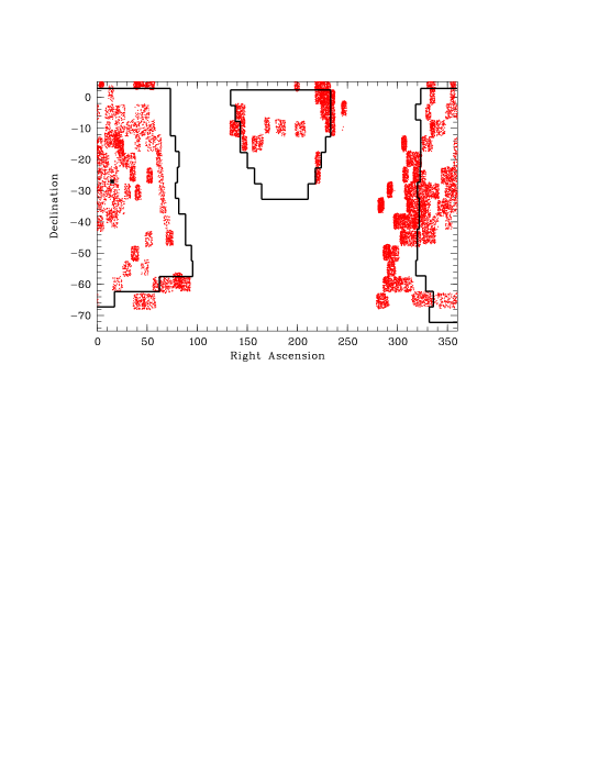
Figure 1: Left panel: Comparison of HES and HK survey volumes; right panel: Comparison of HES area (framed) with HK survey area. Dots denote all HK survey candidates in the southern hemisphere.

By October 1998, just before de-comissioning of the ESO Schmidt telescope, the last HES plate was taken. Today, all 383 plates defining the survey have been scanned in Hamburg using a PDS 1010G microdensitometer. The HES database now consists of $\sim 4,000,000$ digital, extracted, wavelength calibrated, non-overlapping spectra with mean $S/N>5$ (for example spectra see Fig. 2). Note that the elimination of overlapping spectra reduces the survey area from a nominal $9575\,\mbox{deg}^{2}$ to an effective area of $\sim 7600\,\mbox{deg}^{2}$, similar to the total area of the HK survey, where overlapping spectra were not such a severe problem.

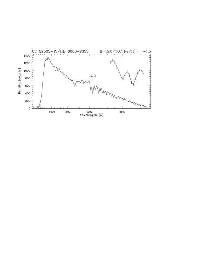
Figure 2: Examples of HES spectra of metal-poor turnoff stars discovered in the HK survey. In the upper right corner of each plot a blow-up of the Ca II H+K region is shown, with an overplot of the pixelwise 1 $\sigma$ noise. Note that the detection of Ca II K in the lower spectrum is not significant. Metal abundances are on the re-calibrated HK survey scale of Beers et al. (1999).

The use of a larger telescope, and a $2$ times lower resolution of the HES compared to the HK survey, results in a limiting magnitude of about $B=17.5$. However, we restricted the selection of metal-poor candidate stars in the HES to $S/N>10$, because it was found that below this $S/N$ level it is extremely difficult to select objects by the absence of individual spectral lines (e.g., the Ca II K line in case of metal-poor stars). In result, the faintest low-metallicity candidates in the HES sample “only” reach $B=17$, about $1.5$ magnitudes deeper than the HK survey. Spectra of bright objects close to saturation where excluded from the search for metal-poor stars, too, because at high illumination, when the characteristic curve of the photographic emulsion gets flatter (at the “shoulder”), the contrast between continuum and spectral lines gets weaker, and apparently all stars have weak lines. The saturation threshold choosen in the HES corresponds to $B\sim 14.0$. Taking the common area of both surveys and their magnitude ranges into account, the HES can increase the total survey volume for metal-poor stars by a factor of 8 compared to the HK survey alone (see also Fig. 1)!

3 Candidate selection

3.1 HK survey

Candidate selection in the HK survey was done by visual inspection of the widened objective-prism spectra with a binocular $10\times$ microscope. Each plate was inspected twice, with a lag time of a month or more between the two inspections. Candidates were identified on the basis of the observed strengths of their Ca II lines (see Fig. 3), and grouped into rough categories based on this criteria (e.g., possibly metal-poor, metal-poor, and extremely metal-poor). Positions of the candidates were noted on the plates, and coordinates for each candidate were measured later (individually, with Grant machines). In this process, a total of about $10\,000$ metal-poor candidates was selected (roughly half of which have had medium-resolution follow-up spectroscopy obtained to date).

Note that since the visual inspection process was made in the absence of any information about the stellar colors (hence temperatures), it was expected that the HK survey candidates would carry a rather severe temperature-related bias, in the sense that cooler metal-deficient stars would likely be missed because of the apparent strength of their Ca II lines at lower temperatures. In addition, stars of high temperature with intermediate abundances would be included in greater number than might be desired because of the apparent weakness of their Ca II lines. These biases become less of a problem at the lowest metallicities, below [Fe/H]$=-2.0$, where the Ca II lines of even quite cool stars are difficult to detect at the resolution of the HK survey.

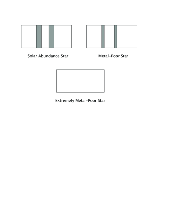
Figure 3: Drawings of HK survey spectra.

3.2 HES

For the present, we have restricted the selection of metal-poor stars in the HES to the color range $0.3<\bv<0.5$, because we decided to focus at first on main-sequence turnoff stars. One of the most interesting applications for these stars is individual age determination based on precise stellar parameters obtained spectroscopically from high-resolution, high $S/N$ observations. However, with a few adaptions the selection procedures described below can easily be used for cooler stars, too, and they will be used for that in the near future, provided that financial support for the continuation of this project is obtained.

Candidate selection in the HES is done by two techniques: The Ca II K index method, and via automatic classification. In the former, stars are selected when their Ca II K line is significantly weaker than “normal.” What is “normal” is determined by a least squares fit of a 2nd order polynomial to the Ca II K index relative to the parameter x_hpp2, which is the half power point of the density distribution of the objective prism spectra in the wavelength range $3890\,\mbox{\AA}<\lambda<5360\,\mbox{\AA}$. x_hpp2 is well-correlated with $\bv$ color, with a $1\,\sigma$ dispersion of $\sim 0.1$ mag. Spectra having a Ca II K index which is more than $3\,\sigma$ below the polynomial fit are selected as metal-poor candidates.

Below we give an outline of metal-poor star selection by automatic classification in the HES. A more detailed description of the method, and all procedures involved (e.g. conversion of flux spectra to artificial objective-prism spectra, automatic feature detection, etc.) will be given in an upcoming paper (Christlieb et al. 2000, in preparation).

For automatic classification we use a learning sample consisting of 45 classes defined by the following grid points:

$$T_{\mbox{\scriptsize eff}} = 5800\,\mbox{K},\,6400\,\mbox{K},\,6800\,\mbox{K}$$

$$\log g = 2.2,\,3.8,\,4.6$$

$$\left[\mbox{Fe/H}\right] = -0.9,\,-1.5,\,-2.1,\,-2.7,\,-3.3$$

The learning sample has been constructed by converting model spectra to simulated objective-prism spectra by reduction of the resolution, and convolution with the effective spectral response of the photographic emulsion and the transmission function of the prism. The model spectra have been kindly provided by J. Reetz and T. Gehren (Universitäts-Sternwarte München, Germany).

Nine automatically detected features are used for classification. These are the strengths of Ca II K, measured by an absorption line fit, and by an index method; the sum of the equivalent widths of H$\beta$, H$\gamma$ and H$\delta$; the half-power point x_hpp2; the three principal components of metal-poor star spectra that account for $90$ % of the variance in the learning sample; and the Strömgren coefficient $c_{1}$, which is directly determined from the objective-prism spectra by integration over the relevant wavelength range. The $c_{1}$ index has been calibrated against HK survey metal-poor stars of Schuster et al. (1996) present on HES plates. The accuracy achieved in this effort is $\sigma_{c_{1}}=0.05$ mag.

The values of the above quantities are organized into “feature vectors” $\vec{x}$. Class-conditional probabilities $p(\vec{x}|\Omega_{i})$ of the learning sample are modelled by multivariate normal distributions, i.e.,

$$p(\vec{x}|\Omega_{i})=\frac{1}{(2\pi)^{d/2}\sqrt{|\Sigma_{i}|}}\exp\left\{-\frac{1}{2}\left(\vec{x}-\vec{\mu}_{i}\right)\Sigma^{-1}_{i}\left(\vec{x}-\vec{\mu}_{i}\right)^{\prime}\right\},$$ (1)

where $i$ denotes class number, $\vec{\mu}_{i}$ the mean feature vector of class $\Omega_{i}$, and $\Sigma_{i}$ the covariance matrix of class $\Omega_{i}$. Using Bayes’ theorem,

$$p(\Omega_{i}|\vec{x})=\frac{p(\Omega_{i})p(\vec{x}|\Omega_{i})}{\sum\limits_{\forall i}p(\Omega_{i})p(\vec{x}|\Omega_{i})},$$

posterior probabilities $p(\Omega_{i}|\vec{x})$ can then be calculated. We assume equal prior probabilities $p(\Omega_{i})$ for all classes present in the learning sample.

A spectrum of unknown class, with given feature vector $\vec{x}$, is classified according to Bayes’ rule: Assign the spectrum to the class with the highest posterior probability $p(\Omega_{i}|\vec{x})$. This rule minimizes the total number of misclassifications if the real distribution of class-conditional probabilities $p(\vec{x}|\Omega_{i})$ is used. It remains to be tested quantitatively if the class-conditional probabilities follow multivariate normal distributions; however, this has been tested qualitatively by visual inspection of the distributions at the computer screen.

Non-mathematically speaking, Bayes’ rule assigns the class with the highest relative resemblance to each spectrum to be classified. However, it is ignorant of the absolute resemblance: A spectrum with feature vector $\vec{x}$ may be assigned to a class with very low posterior probability $p(\Omega_{i}|\vec{x})$, if $p(\Omega_{i}|\vec{x})$ is even lower for all other classes. This means that a class is assigned to all spectra, even to “garbage spectra” which have been disturbed, for instance, by plate artefacts. Therefore, it is useful to apply the following rejection rule: Reject an object from classification to class $\Omega_{i}$, if $a.i.(\Omega_{i};\vec{x})>\beta\,$. The parameter $\beta$ is a threshold to be chosen, and the parameter $a.i.$ is the atypicality index suggested by Aitchison et al. (1977),

$$a.i.(\Omega_{i},\vec{x})=\Gamma\left\{\frac{d}{2};\frac{1}{2}\left(\vec{x}-\vec{\mu}_{i}\right)\Sigma^{-1}_{i}\left(\vec{x}-\vec{\mu}_{i}\right)^{\prime}\right\},$$

where $\Gamma(a;x)$ is the incomplete gamma function and $d$ the number of features used for classification. Use of the above rejection criterion is identical to performing a $\chi^{2}$ test of the null hypothesis $H_{0}$ that an object with feature vector $\vec{x}$ belongs to class $\Omega_{i}$ at significance level $1-\beta$, against the alternative hypothesis $H_{1}$ that it does belong to class $\Omega_{i}$. We reject the null hypotheses, if its significance level is low, i.e., if it is very unlikely that a feature vector $\vec{x}$ is observed for class $\Omega_{i}$, given the multivariate normal distributions (1) are the real distributions of the class-conditional probabilities $p(\vec{x}|\Omega_{i})$.

Note that the automatic classification programs are fed only with a subset of all spectra present on each HES plate. As already mentioned in section 2.2, only spectra with $S/N>10$ and $B\gtrsim 14$ are considered. Moreover, spectra outside of the range $0.3<\bv<0.5$ are excluded, where $\bv$ is known to $\pm 0.1$ mag from the calibration of x_hpp2.

Below we summarize the selection criteria for metal-poor stars in the HES for the selection by automatic classification. Pre-selection of spectra to which automatic classification procedures are applied is done by criteria (1)–(3); (4) and (5) use the results of automatic classification, and (6) is a rejection criterion corresponding to a $\chi^{2}$ test at a $3\,\sigma$ level.

1. $0.3<\bv<0.5$

2. $(S/N)_{\mbox{\scriptsize HES}}>10\Longleftrightarrow B\lesssim 17.0$

3. Photographic density $D$ below saturation threshold

4. $\log g\geq 3.8$

5. $\left[\mbox{Fe/H}\right]\leq-2.7$

6. $a.i.<0.99$.

The final step of the selection is visual inspection of the automatically selected spectra at the computer screen. This step is done for both selections described above. Visual inspection is necessary for identification of plate artefacts (e.g. scratches or emulsion flaws), and for rejection of obviously misclassified spectra, i.e. spectra which clearly show a strong Ca II K line. The remaining candidates are divided into three classes according to the appearance of the Ca II K line region: “class a” candidates show clearly no line; in spectra of “class b” candidates it is unclear if they have a line, and “class c” candidates do show a Ca II K line, but however, a weak one. Typically, only 10 % of the candidates belong to class a or b, 40 % belong to class c, 25 % are misclassifications, and further 25 % are disturbed spectra.

4 Effective yields

As has been pointed out by Beers (2000a), the effective yield (EY) of a detection method is one of the most important properties of a survey for metal-poor stars. EY is defined as follows:

$$\mbox{EY}_{x}:=\frac{N_{\mbox{\footnotesize stars}}\,\,\mbox{with}\,\,\left[\mbox{Fe/H}\right]\,<\,x}{N_{\mbox{\footnotesize stars, observed}}}.$$

When EYs for different surveys are compared, it is crucial to make sure that the comparison is done on the same abundance scale. In case of the HK survey and the HES, it was found that metallicities derived from the first-pass analysis of the HES follow-up spectroscopy are $\sim 0.5$ dex higher on average, than obtained from the Beers et al. (1999) re-calibration. That is,

$$\left[\mbox{Fe/H}\right]_{\mbox{\scriptsize HK}}=\left[\mbox{Fe/H}\right]_{\mbox{\scriptsize HES}}-0.5.$$

This offset of the scales is primarily due to the different temperature scales adopted in the two methods. In the HK survey, effective temperatures are (implicitly) derived from $BV$ photometry, whereas in the HES, Balmer lines are used. The abundance scale previously employed in the HK survey, e.g. in Beers et al. (1992), is known to be an additional $0.2$ dex lower for the lowest metallicity stars (see Beers et al. 2000).

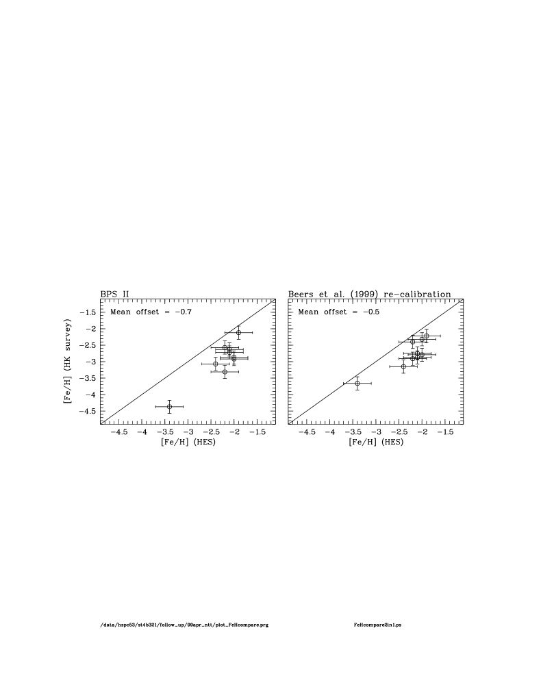
Figure 4: Comparison of HES and HK survey abundance scales. Error bars are $0.2$ dex for the HK survey values, and $0.3$ dex for HES values.

Thus far, only nine stars have been analyzed with both follow-up techniques (see Fig. 4), and there is especially a paucity of comparison objects at $\left[\mbox{Fe/H}\right]_{\mbox{\scriptsize HES}}<-2.5$. However, the derived trend is consistent for all data points. Only turnoff stars have been used in the comparison; therefore, it can not be excluded that the abundance difference is less (or even more) pronounced for cooler stars.

For this discussion, we restrict our EY comparison to turnoff stars in the color range $0.3<\bv<0.5$, and carry out the comparison after an offset of $0.5$ dex has been subtracted from the HES metallicities.

In order to explore what the highest possible EY in the HES is, we observed a sample of 58 HES metal-poor candidates with EMMI at the ESO NTT. The stars have been selected by automatic classification, and have been assigned to candidate classes a or b in the visual inspection. EY of stars at [Fe/H] $<-2.0$ for this sample is 80 % (see Tab. 2). This has to be compared with 11 % or 32 % in the HK survey, depending on whether a pre-selection based on $B-V$ color has been made or not, respectively. We have already obtained data for evaluation of the Ca II K index selection technique in the HES, so that EY of that technique will be known soon.

Survey/selection method	$\mbox{EY}_{-2.0}$	$\mbox{EY}_{-2.5}$
HK survey/without $B-V$ pre-selection	11 %	4 %
HK survey/with $B-V$ pre-selection	32 %	11 %
HES/automatic classification	80 %	27 %

Table 2: Comparison of effective yields (EY) of metal-poor turnoff stars of the HK survey and the HES. [Fe/H] is on the re-calibrated HK survey scale of Beers et al. (1999).

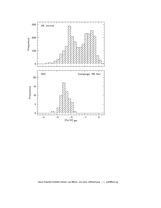
Figure 5: Metallicity distribution function of stars in the color range $0.3<\bv<0.5$ from the HK survey (upper panel), and of a sample of 58 stars selected by automatic classification in the HES.

5 Follow-up techniques

Because of the low quality of objective-prism spectra, and because of their limited spectral resolution, prism surveys for metal-poor stars can only provide, in general, candidate identifications. Note that experiments being conducted by J. Rhee, as part of his thesis work at Michigan State, based on neural-network analysis of line strengths for Ca II H and K obtained directly from automated scans of the HK survey plates, have shown that it might be possible to assign metallicity estimates from the prism spectra themselves, at least in a statistical sense (Rhee et al. 1999). However, in most applications to date, estimates of [Fe/H] and other stellar parameters have to be derived by means of spectroscopic (and, for some techniques, also photometric) follow-up observations. This intermediate step has to be done with some care, because one doesn’t want to spend significant amounts of large telescope time for obtaining high-resolution, high-$S/N$ spectra of “garden variety” stars having as much as $\text@frac{1}{{10}}$ of the solar metal abundance!

5.1 The Ca II K-index and ACF Methods

For candidate low-metallicity stars in the HK survey, medium resolution (1–2 Å) spectroscopy and broadband $BV$ photometry are used to obtain metallicity estimates using two separate techniques. The first technique relies on the assumption that the strength of the Ca II K line tracks the overall stellar [Fe/H], an assumption which is particularly good for stars with [Fe/H] $\leq-1.5$. The second is based on an Auto-Correlation Function (ACF, originally described by Ratnatunga & Freeman 1989) of a stellar spectrum. The ACF method is particularly good for stars with [Fe/H] $>-1.5$, where the Ca II K line begins to saturate with increasing metal abundance. Beers et al. (1999) discuss this calibration, and demonstrate, based on comparisons with some 550 stars with external high-resolution abundance estimates, that these approaches used in combination yield abundance determinations with small scatter (on the order of 0.15–0.20 dex) over the entire range of stellar abundances we expect to find in the Galaxy ($-4.0\leq{\rm[Fe/H]}\leq 0.0$).

In a large collaborative effort involving many astronomers from the U.S., Europe, and Australia, $\sim 4700$ HK survey metal-poor candidates have had spectroscopy obtained, and roughly half of them now have available $BV$ photometry.

5.2 The “all in one shot”-technique

Due to limited telescope time available for follow-up observations, it would be desirable to obtain estimates of stellar parameters, e.g., [Fe/H], $T_{\mbox{\scriptsize eff}}$, and $\log g$, purely spectroscopically, without the need for additional photometry. The first approach attempted with the HES follow-up made use of comparisons with synthetic spectra. However, it turned out that the choice to employ the Mg I b lines as gravity indicators led to a number of difficulties. For example, satisfactory results required high $S/N$ ($>50$) spectra, which are very time consuming to obtain for the fainter stars. Furthermore, at [Fe/H]$\lesssim-2.5$ and turnoff temperatures, Mg I b is so weak that it is not sensitive to gravity anymore. Finally, the comparison of follow-up spectra with synthetic spectra has to be done manually at the computer screen, which is a time sink as well.

As an alternative, the “all in one shot”-technique described below was developed. It is fast, since for each star a single spectrum with $S/N\sim 30$ at Ca II K is all that is required, and data analysis can be done fully automatically.

Spectrophotometry of each candidate is obtained with a wide slit ($\gtrsim 3\times$ seeing disc) rotated to the parallactic angle to avoid atmospheric slit losses. When using EMMI at the 3.5 m ESO NTT, the spectral coverage required for obtaining Strömgren $c_{1}$ coefficients from the spectra ($3200\,\mbox{\AA}<\lambda<4900\,\mbox{\AA}$) limits the maximum possible dispersion to $1.8$ Å per pixel (grating #4), since in the blue arm of EMMI a 1 k CCD is the only available choice. The pixel size is $0\farcs 37$, so that at $\mbox{seeing}<1\farcs 2$, a spectral resolution of $<6$ Å results. Exposure times for obtaining $S/N>30$ at Ca II K are $5$ min for stars of $B<17.0$. In the case where stars exhibit a very weak Ca II K line, as recognized from online-reduced spectra, an additional, longer, exposure with narrow ($1\farcs 0$) slit is obtained. The average total exposure time per object is typically $10$ min, which makes it possible to observe $\sim 30$ metal-poor candidates per night.

The spectra are shifted into the rest frame by cross-correlation with a model spectrum of similar stellar parameters, and applying the appropriate radial velocity correction. Note that the radial velocities derived are not useful measurements in themselves, since the precise position of the object in the (wide) slit is not known. Therefore, zero-point offsets in wavelength can occur.

Three features are used for determination of the stellar parameters [Fe/H], $T_{\mbox{\scriptsize eff}}$, and $\log g$: the Strömgren-coefficient $c_{1}=(u-b)-(v-b)$, the H$\delta$ index HP2, and the Ca II K index KP (for a definition see Beers et al. 1999). The $c_{1}$ index is determined directly from the spectra by multiplication with filter response curves and integration over the appropriate wavelength range (see Fig. 6). The internal accuracy achieved is $\sigma_{c_{1}}=0.022$ mag, which compares favorably with errors from photoelectrically measured indices.

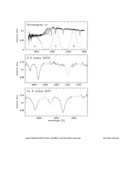
Figure 6: Determination of $c_{1}$, HP2, and KP from photometric, moderate resolution ($\sim 5$ Å) spectra obtained with EMMI attached to the 3.5 m ESO NTT. Dashed lines in the lower two panels indicate continuum and line passbands used for the computation of HP2 and KP, respectively.

Stellar parameters are derived by using the following set of equations:

$$T_{\mbox{\scriptsize eff}} = a_{11}+a_{12}\cdot c_{1}+a_{13}\cdot\mbox{HP2}$$ (2)

$$\log g = a_{21}+a_{22}\cdot c_{1}+a_{23}\cdot\mbox{HP2}$$ (3)

$$\left[\mbox{Fe/H}\right] = a_{31}+a_{32}\cdot\mbox{HP2}+a_{33}\cdot\mbox{KP}$$ (4)

The coefficients $a_{ij}$ have been determined from least squares fits to a dense grid of model spectra, defined by the following grid points:

$$T_{\mbox{\scriptsize eff}} = 5600(200)6800\,\mbox{K}$$

$$\log g = 2.2(0.8)4.6$$

$$\left[\mbox{Fe/H}\right] = -0.9(0.3)-3.6$$

Using equations (2)–(4), it was possible to reproduce the stellar parameters of the model spectrum grid with the following accuracy:

$$\sigma_{T_{\mbox{\tiny eff}}} = 24\,\mbox{K}$$

$$\sigma_{\log g} = 0.21$$

$$\sigma_{\left[\mbox{\tiny Fe/H}\right]} = 0.16.$$

Note that these are internal errors for noise-free spectra. Unfortunately, due to lack of an independent test sample, it is not yet possible to estimate the real accuracy of this approach. However, experience with spectrum synthesis has shown that at the spectral resolution used in the HES follow-up, errors in $\log g$ and [Fe/H] are typically twice as high as the numbers above, and errors in $T_{\mbox{\scriptsize eff}}$ are typically $\sim 200$ K.

6 Discussion and conclusion

We have compared two large, ongoing, surveys for metal-poor stars in the Galactic halo, namely, the HK survey, and the HES. Both surveys are in the position to provide targets for observations with Subaru HDS now. However, follow-up observations of HES stars have just been started, whereas the HK survey has already produced a list of $\sim 4700$ stars with estimates of [Fe/H] typically precise to $\pm 0.2$ dex, on the order of 100 of which exhibit the lowest abundances ever found for stars in the Galaxy.

Selection of metal-poor candidates at the main-sequence turnoff in the HES by automatic classification is $\sim 3\times$/$\sim 7\times$ more efficient as compared to visual inspection in the HK survey with/without pre-selection by $BV$ photometry. This is very remarkable considering the fact that the spectral resolution of the HES is $2\times$ lower than in the HK survey. Reasons for the higher efficiency are the larger spectral coverage of the HES, better quality of the HES spectra, and the automated, quantitative selection, which is probably more precise than the selection by eye. Moreover, we have intentionally observed class a and b candidates only, because we wanted to explore what the maximum possible efficiency is. Simulations we have carried out indicate that, in exchange for a high EY of truly metal-poor stars, one has to sacrifice completeness of the candidate sample on the order of 50 %. Thus, the EY of a selection aimed at compiling a complete sample of metal-poor stars by means of including class c candidates and candidates from complementary selection methods (e.g. the Ca II K index method), too, will be proportionately lower.

The follow-up technique used in the HK survey results in determinations of [Fe/H] precise to $\pm 0.2$ dex; the precision of the HES technique remains to be evaluated. The advantage of the “all in one shot”-technique used in the HES is that no photometry is needed in addition to moderate resolution spectra. However, a drawback is that no useful radial velocities can be measured from spectra obtained with the wide slit, since the object position within the slit is not precisely known, so that unknown zero-point offsets in wavelength occur. We are presently exploring the use of artificial neural network methodology which might be able to recover the required stellar parameters with sufficient accuracy from spectra taken with a narrow slit, so that radial velocity information could be obtained simultaneously (see Qu et al. 1998; Snider et al. 2000).

When compiling target lists for high-resolution observations, combining stars from both surveys, it is important to take into account their different abundance scales. An offset of $0.5$ dex has to be subtracted from [Fe/H] estimates obtained from the HES follow-up, when they are compared with [Fe/H] values derived from the HK survey. Since the limiting magnitude for metal-poor stars in the HES is $\sim 17.0$, and “saturated” objects are excluded from the selection procedure, the HES provides mainly fainter candidates, in the magnitude range $14.0<B<17.0$, whereas the HK survey is able to provide bright candidates in the range $11.0<B<15.5$.

The HES is $\sim 1.5$ mag deeper than the HK survey. Therefore, the former can increase the total survey volume for metal-poor stars by a factor of 8, taking into account common areas and the magnitude ranges of both surveys. We estimate that the total number of stars at [Fe/H]$<-3.0$ known today, $\sim 100$, can be increased to $\sim 800$ by the HES, provided that follow-up observations can be obtained for all candidates. Extension of the procedures described above for the inclusion of cooler stars could easily raise the number of stars with [Fe/H] $<-3.0$ to 1000 or more.

Object lists formed from a combination of targets from both the HK and HES surveys will be able to keep all $8$ m class telescopes busy for at least the next several years. Observations of these stars are sure to provide the astronomical community with many new insights (see Beers, this volume, for an extensive listing). However, a potential “metal-poor star disaster” is only a few years away, in the sense that a much larger database of candidates will be necessary to address the many new questions which are sure to arise from the first-pass 8 m-class telescope follow-ups (see Beers 2000b). Now is the time to expand efforts to obtain large numbers of new metal-deficient stars from follow-up of the HES and HK survey candidates!

References

- (1)
- Aitchison et al. (1977) Aitchison, J., Habbema, J. & Kay, J. (1977), ‘A Critical Comparison of Two Methods of Statistical Discrimination’, Applied Statistics 26, 15–25.
- Beers (2000a) Beers, T. C. (2000a), Population III by popular demand – progress and previews, in A. Weiss, T. Abel & V. Hill, eds, ‘The First Stars, Proceedings of the second MPA/ESO workshop’, Springer, Heidelberg, in press. (astro-ph/9911171).
- Beers (2000b) Beers, T. C. (2000b), Observational constraints on the Nature of the first stars – final comments, in A. Weiss, T. Abel & V. Hill, eds, ‘The First Stars, Proceedings of the second MPA/ESO workshop’, Springer, Heidelberg, in press.
- Beers et al. (1985) Beers, T. C., Preston, G. W. & Shectman, S. A. (1985), ‘A search for stars of very low metal abundance. I.’, AJ 90, 2089–2102.
- Beers et al. (1992) Beers, T. C., Preston, G. W. & Shectman, S. A. (1992), ‘A search for stars of very low metal abundance. II.’, AJ 103, 1987–2034.
- Beers et al. (1999) Beers, T. C., Rossi, S., Norris, J. E., Ryan, S. G. & Shefler, T. (1999), ‘Estimation of Stellar Metal Abundance. II. A Recalibration of the Ca II K Technique, and the Autocorrelation Function Method’, AJ 117, 981–1009.
- Beers et al. (2000) Beers, T. C., Chiba, M., Yoshii, Y., Platais, I., Hanson, R. B., Fuchs, B. & Rossi, S. (2000), ‘Kinematics of Metal-Poor Stars in the Galaxy. II. Proper Motions for a Large Non-Kinematically Selected Sample’, AJ, submitted.
- Qu et al. (1998) Qu, Y., Snider, S., von Hippel, T., Sneden, C., Lambert, D., Beers, T. & Rossi, S. (1998), ‘Neural Network Techniques Applied to Low Resolution Spectra of Halo Stars’, BAAS 193, #44.09.
- Ratnatunga & Freeman (1989) Ratnatunga, K. U. & Freeman, K. C. (1989), ‘Field K Giants in the Galactic Halo. II. Improved Abundance and Kinematic Parameters’, ApJ 339, 126–148.
- Rhee et al. (1999) Rhee, J., Beers, T. C. & Irwin, M. J. (1999), ‘Automatic Identification, Classification, and Abundance Estimation for Metal-Poor Stars in the Galaxy from Objective-Prism Spectroscopy Using a Neural Network Analysis’, BAAS 31, 971.
- Schuster et al. (1996) Schuster, W. J., Nissen, P. E., Parrao, L., Beers, T. C. & Overgaard, L. (1996), ‘uvby- photometry of high-velocity and metal-poor stars. VIII. Stars of very low metal abundance.’, A&AS 117, 317–334.
- Snider et al. (2000) Snider, S., Qu, Y., Allende-Prieto, C., von Hippel, T., Beers, T. C., Sneden, C., Lambert, D. L. & Rossi, S. (2000), Teff, log g, [Fe/H] Classification of Low-Resolution Stellar Spectra Using Artificial Neural Networks, in ‘11th Cambridge Workshop on Cool Stars’, in press.
- Wisotzki et al. (1996) Wisotzki, L., Köhler, T., Groote, D. & Reimers, D. (1996), ‘The Hamburg/ESO survey for bright QSOs I. Survey design and candidate selection procedure’, A&AS 115, 227–233.
- Wisotzki et al. (2000) Wisotzki, L., Christlieb, N., Bade, N., Beckmann, V., Köhler, T., Vanelle, C. & Reimers, D. (2000), ‘The Hamburg/ESO survey for bright QSOs. III. A large flux-limited sample of QSOs’, A&AS, submitted.