Asteroseismology and Oblique Pulsator Model of $\beta$ Cephei

Abstract

We discuss the oscillation features of $\beta$ Cephei, which is a magnetic star in which the magnetic axis seems to be oblique to the rotation axis. We interpret the observed equi-distant fine structure of the frequency spectrum as a manifestation of a magnetic perturbation of an eigenmode, which would be a radial mode in the absence of the magnetic field. Besides these frequency components, we interpret another peak in the frequency spectrum as an independent quadrupole mode. By this mode identification, we deduce the mass, the evolutionary stage, the rotational frequency, the magnetic field strength, and the geometrical configuration of $\beta$ Cephei.

and

1 Introduction

Beta Cephei (B1III, ${\rm V}=3.2$, $V_{\rm e}\sin i=25$ km/s) is the prototype of a group of early-type pulsating stars. Since many of the $\beta$ Cephei-type stars show multi-periodic pulsations, it is expected that a lot of information can be extracted from the pulsations of these stars. Recently, Aerts et al. (1994) and Telting, Aerts, & Mathias (1997) investigated the line-profile variability of $\beta$ Cephei in detail, by means of an extensive data set of high-resolution, high S/N spectra obtained at the Observatoire de Haute Provence during one month, and deduced that the variations show periodicity with at least five frequencies. The frequencies obtained by them from the intensity variation in the Si III $\lambda$ 4574 line are listed in table 1. Note that three frequencies among them ($f_{3}$, $f_{4}$, and $f_{5}$) are separated from the main frequency $f_{1}=5.250$ day^-1 by $-2/6$ day^-1, $-1/6$ day^-1, and $+1/6$ day^-1, respectively. Hence, we regard that the four peaks (and the small peak at $f_{1}+2/6$ day^-1) are a part of a frequency quintuplet with equal spacing. The central frequency $f_{1}$ has been identified as the radial pulsation mode by Aerts et al. (1994) and by Telting et al. (1997). The second highest peak in the periodogram, $f_{2}$ seems to be an independent mode, and has been identified as an $\ell=2$ mode by Telting et al. (1997).

Table 1: Observed frequencies of spectral line variations.

	Frequencies (day-1)	Amplitude
$f_{3}$	4.923	$6.89\times 10^{-4}$
$f_{4}$	5.082	$1.10\times 10^{-3}$
$f_{1}$	5.250	$1.00$
$f_{2}$	5.380	$1.41\times 10^{-3}$
$f_{5}$	5.417	$1.40\times 10^{-3}$
$f_{6}$?	5.583	$1.62\times 10^{-4}$

Besides the pulsations in the luminosity and in the velocity field, a magnetic field has been reported at several occasions in the past. For a compilation of these results, see Veen (1993). No clear periodicity was found in these old measurements. Very recently however, Henrichs et al. (1999) re-measured the magnetic field and found a clearly variable field with a period of 12 days and a semi-amplitude of $90\pm 6\,$G. The UV wind lines of this star also reveal a periodic variation with both a 6 day and a 12 day periodic component (Henrichs et al. 1993), the 6 day period clearly being the dominant variation. From these results, it is concluded that the magnetic field of $\beta$ Cephei is oblique to the rotation axis.

In this paper, we try to understand the cause of the quintuplet and to extract information on the evolutionary stage and the geometrical configuration of $\beta$ Cephei by using the oscillation data and the most recent magnetic data. A previous similar study was presented in Shibahashi & Aerts (1998) but they still used the older magnetic field measurements.

2 Oscillations of a Rotating Magnetic Star

Henrichs et al. (1999) find a variable magnetic field with a mean value of only $0\pm 5\,$G. We assume here that the dominant component of the weak magnetic field is dipolar. Being influenced by such a magnetic field, the eigenmode, which would be a pure radial mode in the absence of a magnetic field, is deformed to have an axially symmetric quadrupole component, whose symmetric axis coincides with the magnetic axis. Hence, the eigenfunction at the surface is characterized by means of a superposition of the spherical harmonic with $\ell=m=0$ and that of $\ell=2$ and $m=0$ with respect to the magnetic axis (Shibahashi 1994, Shibahashi & Takata 1995); i.e.,

$$\left[Y_{0}^{0}(\theta_{B},\phi_{B})+\alpha Y_{2}^{0}(\theta_{B},\phi_{B})\right]\exp(i\omega t),$$ (1)

where $\alpha$ is determined by the magnetic field of the star and the unperturbed eigenfunction of the mode. Since we are assuming that the magnetic axis is oblique to the rotation axis, the aspect angle of the pulsation axis varies with the rotation of the star. Therefore, the contribution of the quadrupole component of the eigenfunction to the apparent intensity variation changes with time and produces a quintuplet fine structure with an equal spacing of the rotation frequency in the power spectrum. Mathematically, a spherical harmonic expressed in the spherical coordinates with respect to the magnetic axis $(\theta_{B},\phi_{B})$ is written in terms of $(2\ell+1)$ spherical harmonics of the same degree $\ell$ with respect to the spherical coordinates $(\theta_{L},\phi_{L})$:

$$Y_{\ell}^{m}(\theta_{B},\phi_{B}) = \sum_{m^{\prime}=-\ell}^{\ell}\sum_{m^{\prime\prime}=-\ell}^{\ell}(-1)^{m^{\prime}}d_{0m^{\prime}}^{(\ell)}(\beta)d_{m^{\prime}m^{\prime\prime}}^{(\ell)}(i)$$ (2)

$$Y_{\ell}^{m^{\prime\prime}}(\theta_{L},\phi_{L})\exp(-im^{\prime}\Omega t),$$

where $\{d_{mm^{\prime}}^{(\ell)}(\beta)\}$ and $\{d_{m^{\prime}m^{\prime\prime}}^{(\ell)}(i)\}$ are the matrices to transform the spherical harmonics expressed in terms of the spherical coordinates with respect to the magnetic axis, to those expressed in terms of the spherical coordinates with respect to the line-of-sight. The explicit form of $\{d_{mm^{\prime}}^{(\ell)}(\beta)\}$ for $\ell=2$ can be found in Kurtz et al. (1989). The angles $\beta,i\in[0^{\circ},180^{\circ}]$ are the angle between the magnetic axis and the rotation axis and that between the line-of-sight and the rotation axis, respectively. The observable variation is obtained by integrating equation (1) over the visible disc ($\theta_{L}=[0,\pi/2]$ and $\phi_{L}=[0,2\pi]$) after substituting equation (2) into equation (1). Since the integral with respect to $\phi_{L}$ becomes zero unless $m^{\prime\prime}=0$, the amplitude of the component at $\omega+m^{\prime}\Omega$ is proportional to $d_{0m^{\prime}}^{(2)}(\beta)d_{m^{\prime}0}^{(2)}(i)$ (Shibahashi 1986). If an additional quadrupole component of the magnetic field is taken into account, the eigenfunction is deformed to have $\ell=1$, $\ell=3$, and $\ell=4$ components as well and then the expected power spectrum becomes a nonuplet (a 9-fold multiplet) rather than a quintuplet (Shibahashi 1994, Takata & Shibahashi 1994). The additional outer side-components are due to the $\ell=3$ and $\ell=4$ components, and hence their amplitudes are expected to be much smaller than the central five components.

3 Deduction of $\tan\beta$ and $\tan i$

If the star is rotating with a period of 6 days, then the power spectrum of the eigenmode, which would be the radial mode in the absence of the magnetic field, is expected to reveal a quintuplet with an equal spacing of 1/6 day^-1. This can be explained by the observed quintuplet fine structure of ${f_{1}}$, $f_{3}$, $f_{4}$, $f_{5}$, and an additional very small peak in the power spectrum (which we call $f_{6}$). The relative ratios of the side-peaks’ amplitudes to the central peak amplitude depend on the strength of the magnetic field. On the other hand, the relative ratios among the side-peak amplitudes depend on the angles $\beta$ and $i$. By analyzing them, we can determine these angles. If we write the amplitude of the component at $\omega+m^{\prime}\Omega$ as $A_{m^{\prime}}$, then $(A_{2}+A_{-2})/(A_{1}+A_{-1})$ is given by (Shibahashi 1986)

$${{A_{2}+A_{-2}}\over{A_{1}+A_{-1}}}=\left|{{d_{02}^{(2)}(\beta)d_{20}^{(2)}(i)}\over{d_{01}^{(2)}(\beta)d_{10}^{(2)}(i)}}\right|={{1}\over{4}}\left|\tan\beta\tan i\right|.$$ (3)

Substitution of the observed amplitudes into the above equation leads to $|\tan\beta\tan i|\simeq 2.2$, where we have used $A_{2}=A_{-2}$ since the presence of a frequency peak at $f_{6}$ is not well established. The factor $\tan\beta\tan i$ can be independently estimated from the variation in the magnetic field strength. Let $r$ be the ratio between the apparent minimum and the maximum of the field strength,

$$r\equiv{{B_{\rm obs,min}}\over{B_{\rm obs,max}}}.$$ (4)

Then it is related with the geometrical configuration by (Stibbs 1950)

$$\tan\beta\tan i={{1-r}\over{1+r}}.$$ (5)

Substitution of the observed values gathered by Henrichs et al. (1999) together with their error, $r\in[-2.5,-0.6]$, leads to $\tan\beta\tan i\in[-\infty,-2.3]$ or $[4.1,\infty]$. This result is seemingly in contradiction with the one derived from the amplitude ratio, but we will show in the Sect. 5 that the two estimates are compatible with each other and point to almost the same geometry.

4 Identification of the Evolutionary Stage

The second highest peak $f_{2}$ in the power spectrum has been identified by Telting et al. (1997) as a mode with $\ell=2$ and $m=+1$. Telting et al. (1997) have chosen the rotation axis as the symmetry axis of the pulsation in their work. If the magnetic effects on the pulsation dominate over the effects due to the Coriolis force, as applies here, the symmetry axis of the eigenfunction is the magnetic axis rather than the rotation axis. Following Telting et al.’s (1997) mode identification, we assume that $f_{2}$ belongs to a quadrupole ($\ell=2$) mode, but we assume $m=0$ with respect to the magnetic axis. As will be shown later, the following conclusion about the evolutionary stage is the same even in the case of $m\neq 0$. Under the influence of the magnetic field, this mode is no longer described by a single spherical harmonic of $\ell=2$ and $m=0$, and it is deformed to have components of some other $\ell$. However, the fine structure of this mode is expected to be difficult to detect, since the amplitude of the $f_{2}$ component itself is small.

Since we have two independent frequencies, $f_{1}$ and $f_{2}$, we can identify the evolutionary stage of the star. Figure 1 shows the frequency variation of a $10M_{\odot}$ star. The left panel shows the radial mode frequency variation, while the right panel shows the case of $\ell=2$ modes. As the star evolves from the zero age main sequency, its radius increases and hence the frequency decreases. The situation changes during the contraction phase when hydrogen is exhausted in the stellar center, and the frequency increases again in the hydrogen shell-burning phase. The frequency variation of the $\ell=2$ mode is more complicated because the $\mu$-gradient zone around the convective core grows with evolution as a consequence of conversion of hydrogen into helium. The frequencies of the modes trapped there become higher. When the frequencies of two modes happen to be very close, they never degenerate but repel each other. This is known as “avoided crossing” (cf. Unno et al. 1989).

Figure 1: Frequency variation of radial modes (left panel) and $\ell=2$ modes (right panel) of a $10M_{\odot}$ star with stellar evolution. The vertical scale is in unit of day^-1, and the horizontal scale shows the model numbers (Model 1 is the zero-age main-sequence star, and Model 33 is the model at the turning point on the HR-diagram.). The solid lines indicate the observed frequencies $f_{1}$ (left panel) and $f_{2}$ (right panel).

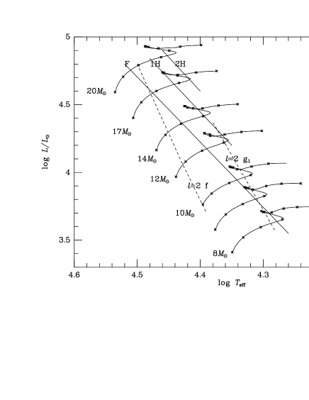
By sweeping out evolutionary models of various masses, we search for stellar models whose radial and quadrupole mode eigenfrequencies coincide with the observed frequency $f_{1}$ and $f_{2}$. Figure 2 shows the series of these models on the HR diagram, calculated by using Pacyński’s (1970) program ($X_{0}=0.73$ and $Z_{0}=0.02$). The two dashed lines show the models of which the quadrupole mode has the same frequency as $f_{2}$, and the solid lines show the models whose radial mode frequency coincides with $f_{1}$. $\beta$ Cephei must be on one of the crossing points of the solid lines and the dashed lines. The candidate is (i) a $\sim 18M_{\odot}$ star at the middle of the hydrogen core-burning phase, or (ii) a $\sim 12M_{\odot}$ star near the turning point, or (iii) a $\sim 9M_{\odot}$ star at the late stage of the hydrogen core-burning phase.

Figure 2: The HR-diagram of 8–20 $M_{\odot}$ stars. The tick marks on each of the evolutionary tracks indicate Models 1, 10, 20, $\cdots$. The stars whose radial mode frequency coincides with the observed frequency $f_{1}$ are connected with the solid lines, and those whose quadrupole mode frequency matches with $f_{2}$ are shown by the dashed lines. The crossing points of the solid and dashed lines are the candidate locations for $\beta$ Cephei on the HR-diagram.

5 Deduction of $i$ and $\beta$

The oscillation mode $f_{1}$ is identified as the radial fundamental mode in the case (i) or (iii) in the previous section. On the other hand, it is identified as the radial first harmonic in the case (ii). First, let us consider the case (iii). The radius of the star for the case (iii) is estimated from the stellar evolution calculation as $R\simeq 6.5R_{\odot}$. Since in our consideration $2\pi/\Omega=6$ days and $V_{\rm e}\sin i\simeq 25$ km/s, this means $i\simeq 30^{\circ}$ or $150^{\circ}$. Combining this with the first estimate of $|\tan\beta\tan i|\simeq 2.2$ deduced from the power spectrum, we obtain $\beta\simeq 75^{\circ}$ or $105^{\circ}$. The estimate $\tan\beta\tan i\simeq-6.14$ deduced from the recent magnetic field measurements results in $\beta\simeq 95^{\circ}$. We obtain that the solutions from both estimates of $\tan\beta\tan i$ point towards an almost equal geometry. The orientation of the magnetic axis can only be derived from the measurements of the magnetic field. We conclude that the angle between the rotation axis and the magnetic axis amounts to some $100^{\circ}$ in $\beta$ Cephei in the case of scenario (iii).

If we take the case (ii), the radius of the star is larger than the case (iii) ($R\simeq 8.5R_{\odot}$), and hence $i$ becomes smaller ($i\simeq 20^{\circ}$ or $i\simeq 160^{\circ}$) and $\beta$ becomes close to $90^{\circ}$ ($\beta\simeq 80^{\circ}$ or $100^{\circ}$ if $|\tan\beta\tan i|\simeq 2.2$ and $\beta\simeq 93^{\circ}$ if $\tan\beta\tan i\simeq-6.1$). Though the case (ii) cannot be ruled out, we think the case (iii) is more likely because the radial fundamental mode is more easily excited. The case (i) seems unlikely because of a high mass required.

In the case of $m\neq 0$, the frequency of the quadrupole mode is shifted by the Coriolis force by $mC\Omega\cos\beta$ (Shibahashi & Takata 1993). Here $C$ is determined by the equilibrium structure and the eigenfunction, and it is of the order of $\sim 0.1$ for the low order p-modes of $\ell=2$. Since $|\cos\beta|\sim 0.17$, the frequency shift due to the Coriolis force is so small that we do not need to change the conclusion about the evolutionary stage discussed in the previous section.

We have adopted the case (iii), and have calculated the theoretically expected power spectra and compared them with the observations. Figure 3 was calculated with an assumption of $B_{\rm obs,max}=90$ G, $i=30^{\circ}$, and $\beta=95^{\circ}$ (the upper panel) and $\beta=105^{\circ}$ (the lower panel). The magnetic field was assumed to be mainly dipolar with a 10% contribution from a quadrupole component. (Note that the combination of $i$ and $\beta$ is reversible.) Figure 3 resembles the observed power spectrum, and it implies that our identification of the pulsation modes, the evolutionary stage of the star, and the geometrical configuration are reasonable.

Figure 3: Theoretically expected power spectrum. The model is a $9M_{\odot}$ star at the late stage of the hydrogen core-burning phase. The mode $f_{1}$ is identified as the radial fundamental mode. The angle between the rotation axis and the line of sight is assumed to be $30^{\circ}$ and the magnetic axis is assumed to be inclined to the rotation axis by $95^{\circ}$ (upper panel) and $105^{\circ}$ (lower panel). The magnetic field strength is assumed to be $B_{\rm obs,max}=90$ G, and the field is assumed to be a dipole + quadrupole field, and the latter contribution is 10%.

6 Discussion

The UV line variation of $\beta$ Cephei implies that the rotation period is either 6 days or 12 days with the latter being more likely as the UV line equivalent-width reveals a variation with alternating deep and less-deep minima (Henrichs et al. 1993). Based on this observation, Henrichs et al. (1999) prefer an oblique rotator model with a dipolar magnetic field and with a rotation period of 12 days, the more so since this is the main period found in their 14 recent observations of the averaged value of the magnetic field over the stellar disk. Such a model can explain the UV data if an equator-on view is assumed. However, if the rotation period is 12 days and the magnetic field is a pure dipole, then the power spectrum of the line-profile variations must show a quintuplet of an equal spacing of 1/12 day^-1 for $i\neq 90^{\circ}$ and $\beta\neq 90^{\circ}$, or a triplet of an equal spacing of 1/6 day^-1 for $i=90^{\circ}$ or $\beta=90^{\circ}$; a quintuplet fine structure of an equal spacing of 1/6 day^-1 is in that case unrealistic.

In order to get an apparent quintuplet of the spacing of 1/6 day^-1 with the rotation period of 12 days from the oblique pulsator model, we have to assume that the magnetic field is almost entirely quadrupolar rather than dipolar and choose an appropriate geometrical configuration to give only the five components among the nonuplet fine structure of the visible amplitude. The former condition is necessary, because, otherwise, the eigenfunction would have an $\ell=1$ component, which would induce a pair of peaks separated from the central peak in the power spectrum by 1/12 day^-1. In the case of a pure quadrupole magnetic field, the eigenfunction is characterized by means of a superposition of the spherical harmonic with $\ell=m=0$ and those of $\ell=2$ and $m=0$ and $\ell=4$ and $m=0$ (Takata & Shibahashi 1994).The $\ell=4$ component induces a nonuplet fine structure. But, in the case of $i\simeq 90^{\circ}$ or $\beta\simeq 90^{\circ}$, both of the amplitudes at $\omega\pm\Omega$ and at $\omega\pm 3\Omega$ happen to become much smaller than those at $\omega\pm 2\Omega$ and $\omega\pm 4\Omega$, and the fine structure looks like a quintuplet with an equal spacing of 1/6 day^-1 (see figure 4). The combination of $2\pi/\Omega=$ 12 days and $V_{\rm e}\sin i\simeq 25$ km/s indeed leads to $i\simeq 90^{\circ}$, and one might consider that this would be favorable to explain the apparent quintuplet fine structure. However, in the case of a pure quadrupole magnetic field, the observed magnetic field strength should vary as

$$B_{\rm obs}\propto P_{2}(\cos\Theta)\propto 3\cos^{2}\Theta-1,$$ (6)

where

$$\cos\Theta=\cos\beta\cos i-\sin\beta\sin i\cos\Omega t.$$ (7)

Then, in the case of $i\simeq 90^{\circ}$, the observed magnetic field strength is expected to vary with a period of 6 days rather than 12 days, and this is in contradiction with the observation (Henrichs et al. 1999).

Figure 4: The same as figure 3 but for the almost quadrupole magnetic field and $i=90^{\circ}$ and $\beta=50^{\circ}$. The value of $i$ has been chosen so that it is consistent with $R\simeq 6.5R_{\odot}$, $2\pi/\Omega$ = 12 days and $V_{\rm e}\sin i=25$ km/s. The value of $\beta$ has been chosen so that $r\simeq-1.4$ with an assumption of a quadrupole magnetic field and $i=90^{\circ}$. The dipole field contribution is assumed to be only 0.01%.

In order to solve the controversy about the rotation period of the star, it is highly desirable that numerous new magnetic field measurements be performed over a much longer time base than achieved so far. We note that the older magnetic field measurements pointed towards very different values of the mean field, ranging from 70 G up to 800 G (Rudy & Kemp 1978, Veen 1993). The new data obtained by Henrichs et al. (1999), however, are of much better quality. It would be extremely important to confirm the results by Henrichs et al. (1999) and to achieve a better precision of the strength and the geometry of the magnetic field. This would allow a critical evaluation of the current theory of pulsations in hot magnetic stars.