Best Unbiased Estimators for the Three-Point Correlators of the Cosmic Microwave Background Radiation

Abstract

Measuring the three-point correlators of the Cosmic Microwave Background (CMB) anisotropies could help to get a handle on the level of non-Gaussianity present in the observational datasets and therefore would strongly constrain models of the early Universe. However, typically, the expected non-Gaussian signal is very small. Therefore, one has to face the problem of extracting it from the noise, in particular from the ‘cosmic variance’ noise. For this purpose, one has to construct the best unbiased estimators for the three-point correlators that are needed for concrete detections of non-Gaussian features. In this article, we study this problem for both the CMB third moment and the CMB angular bispectrum. We emphasize that the knowledge of the best estimator for the former does not permit one to infer the best estimator for the latter and vice versa. We present the corresponding best unbiased estimators in both cases and compute their corresponding cosmic variances.

1. Introduction

The Cosmic Microwave Background (CMB) has been recognized as one of the best tools for studying the early Universe (e.g. Scott (1999)). In particular, the statistical properties of the CMB anisotropies are a powerful means to discriminate amongst the possible scenarios. This is because, in general, different models predict different statistical properties. For example, the simplest models of inflation predict that the temperature anisotropies should obey a Gaussian statistics and therefore any non-vanishing measurement of a three-point correlator (in a sense to be precised below) would automatically ruled out such models, a very interesting result indeed.

From a practical point of view, measuring any non-Gaussianity in the data is a very difficult task since the signal is typically very small. Of course, this signal should be compared to the noise and what really matters is the signal to noise ratio. The noise can have many different origins including instrumental errors, foregrounds contamination or incomplete sky coverage. Another source of error is the so-called ‘cosmic variance’. Roughly speaking, it comes from the fact that we only have access to one realization of the temperature anisotropies whereas theoretical predictions are expressed through ensemble averages. In a Gaussian model, for example, the mean value of any three-point correlator has to vanish but this does not guarantee that a concrete detection of a non-zero signal on the sky would be in contradiction with the model (Scaramella & Vittorio (1991); Srednicki (1993)). The important point is that the cosmic variance can dominate the other sources of error, as this is in fact the case for the two-point correlators on large angular scales. Therefore, if one wants to unveil non-Gaussianity, it is necessary to address the cosmic variance problem for the three-point correlators. The usual way to deal with this problem is to construct estimators by performing spatial averages on the celestial sphere and to find the one which has the smallest possible variance. The aim of this paper is then to find the best unbiased estimators both for the third moment $\bigl{\langle}a_{\ell_{1}}^{m_{1}}a_{\ell_{2}}^{m_{2}}a_{\ell_{3}}^{m_{3}}\bigr{\rangle}$ and for the angular bispectrum ${\cal C}_{\ell_{1}\ell_{2}\ell_{3}}$ and to display the corresponding cosmic variances.

Recently, there has been a lot of activity in the subject triggered by the finding that non-Gaussianities are present in the 4-yr COBE-DMR data (Ferreira et al. (1998); Pando et al. (1998)). Further analyses have confirmed this result (e.g. Bromley & Tegmark (1999)). However, soon after, it was demonstrated by Banday et al. (1999) that the non-Gaussian signal is driven by the 53 GHz data. This systematic artifact in the CMB maps rejects a possible cosmological origin. More generally, it is clear that the presence of foregrounds (Bouchet & Gispert (1999); Tegmark et al. (1999)) renders difficult the detection of a genuine non-Gaussian signal. Nevertheless, one should expect non-Gaussian features to be present in the CMB anisotropy datasets. These could be produced in the early Universe during inflation either because the initial conditions are non-Gaussian themselves [i.e. the quantum initial state is not the vacuum (Martin et al. (1999); Contaldi et al. (1999))] or owing to the existence of couplings between different perturbation modes at the non-linear level (Gangui et al. (1994); Gangui (1994); Linde & Mukhanov (1997)). In the context of slow-roll inflation, the CMB bispectrum has recently been studied in (Gangui & Martin (2000); Wang & Kamionkowski (2000)). Even if non-Gaussianities are not primordial in origin, they will nevertheless arise during later stages of evolution. In this context, the Rees-Sciama effect will build up a small but non-vanishing signal (Luo & Schramm (1993); Mollerach et al. (1995); Munshi et al. (1995)). Also, cosmic topological defects of the vacuum, like strings and textures, are amongst the best motivated sources for non-Gaussian features (Bouchet et al. (1988); Ferreira & Magueijo (1997); Avelino et al. (1998); Gangui & Perivolaropoulos (1995); Gangui & Mollerach (1996)). Regarding secondary sources, Goldberg & Spergel (1999) and Spergel & Goldberg (1999) have recently calculated the angular bispectrum due to second order gravitational effects like the correlation of lensing of CMB photons and secondary anisotropies coming from the Integrated Sachs Wolfe effect and thermal Sunyaev-Zel’dovich effect. In the same line, Cooray and Hu (1999) have taken into account further additional contributions to the bispectrum in the presence of reionization. Other approaches to the study of non-Gaussian features include preferred-direction statistics for sky maps (Bunn & Scott (1999)), the three-point correlation function (Falk et al. (1993); Hinshaw et al. (1994); Gangui et al. (1994); Hinshaw et al. (1995)), lensing statistics (Bernardeau (1997); Winitzki (1998); Zaldarriaga (1999)), the genus and Euler-Poincaré statistics (Coles (1989); Gott et al. (1990); Smoot (1999)), peak statistics (Bond & Efstathiou (1987); Kogut et al. (1995, 1996)), correlation function of peaks (Heavens & Sheth (1999)), Minkowski functionals (Winitzki & Kosowsky (1998)) and wavelet analyses (Popa (1998); Hobson et al. (1998)).

This article is organized as follows. In the next section, the general strategy for finding best estimators is exposed. As a warm up, in the third section, we implement this strategy for the two-point correlators. The fourth section is the core of the article. There we explicitly derive, for the first time, the best unbiased estimator for the angular bispectrum and show its corresponding variance. Except for an overall normalization factor, this estimator turns out to be the one already employed by Ferreira et al. (1998) and other authors recently. Our result places their choice on a firm basis. Next, we find the expression for the best unbiased estimator for the third moment. An earlier study was performed in (Heavens (1998)); however, our findings go beyond the results obtained in that article and, moreover, are explicit. Moreover, we present its corresponding variance. In addition, we also emphasize that the knowledge of the best estimator for the third moment does not allow one to infer the best estimator for the angular bispectrum and vice versa. In the last section, we briefly present our main conclusions. We finish up with a short Appendix which includes formulae related to the inverse two-point correlation function.

2. General strategy for finding the best estimator

In this section, we expose the cosmic variance problem from the viewpoint of the theory of cosmological perturbations of quantum-mechanical origin and describe the method of the best unbiased estimators. This theory rests on the principles of general relativity and quantum field theory. At the beginning of the inflationary phase (Guth (1981); Linde 1983a ; Albrecht & Steinhardt (1982); Linde 1983b ) the Friedmann-Lemaître-Robertson-Walker background spacetime already behaves classically whereas the excitations of the metric around this background are still quantum mechanical in nature. Technically, this means that the perturbed metric must be considered as a quantum operator. This operator either represents density perturbations or gravitational waves. In each case, the quantization can be carried out in a consistent way (Mukhanov & Chibisov (1981); Hawking (1982); Starobinsky (1982); Bardeen et al. (1983); Mukhanov et al. (1992); Grishchuk (1993); Martin & Schwarz (1998), 1999). Then, the (zero-point) quantum fluctuations, which are the seeds of the cosmological perturbations, are amplified during inflation owing to the particle-creation phenomenon or squeezing effect (Grishchuk & Sidorov (1990)). Next, these primordial fluctuations give rise to the large scale structures and to the CMB anisotropies observed today in our Universe.

One should also discuss the choice of the quantum state in which the metric operator is placed. Obviously, it is not possible to prepare the initial state of the Universe and therefore the choice of the quantum state of the perturbations is a priori free unless some theory of the initial conditions is provided [for example, quantum cosmology (Halliwell (1989))]. Usually, it is assumed that the initial state is the vacuum although different hypothesis are possible (Brandenberger & Hill (1986); Martin et al. (1999); Contaldi et al. (1999)). If the initial state is the vacuum, then the corresponding statistical properties are Gaussian. This is because the ground-state wave function of an harmonic oscillator is a Gaussian. It is possible to avoid this general conclusion either by considering non-linear cosmological perturbations or by assuming that the initial state is a non-vacuum state. We have recently investigated the first possibility in (Gangui & Martin (2000)). The second possibility has been studied by Martin et al. (1999). In the latter case, non-Gaussianity is likely to be significant only for relatively small angular scales.

It should be emphasized that the mechanism described previously is deeply rooted in the quantum-mechanical nature of the gravitational field. The observable quantities calculated in this framework are always proportional to the Planck length. In other words, if observations confirm the full set of inflationary predictions then the fact that ${\rm\delta}T/T\neq 0$ would be a direct observational consequence of quantum gravity.

The quantum-mechanical origin of the anisotropies in the framework of inflation raises also profound problems of interpretation. One should not think that these problems are purely theoretical. On the contrary, they have consequences with regards to the experimental strategy that one should follow in order to extract as much informations as possible from the data. The fluctuations in the CMB effective temperature are linked to the perturbed metric as shown for the first time by Sachs and Wolfe. Therefore, the fact that the perturbed metric is an operator implies that the primordial fluctuations in the temperature must also be considered as a quantum operator. The observables are often expressed as $n$-point correlation functions of the operator $\hat{\Delta}({\bf e})\equiv\hat{\delta T/T}({\bf e})$ in the arbitrary state $|\Psi\rangle$

$$\xi_{n}({\bf e}_{1},\cdots,{\bf e}_{n})\equiv\langle\Psi|\hat{\Delta}({\bf e}_{1})\cdots\hat{\Delta}({\bf e}_{n})|\Psi\rangle,$$ (1)

where ${\bf e}_{i}$’s are arbitrary directions on the celestial sphere. In the following, we will also use the notation $\xi({\bf e}_{1}\!\cdot\!{\bf e}_{2})\equiv\xi_{2}({\bf e}_{1},{\bf e}_{2})$. According to the postulates of quantum mechanics, the previous theoretical predictions should be confronted to experiment in the following way. The same experiment should be performed $N$ times giving each time different outcomes $q_{i}$. If the quantity $(1/N)\sum_{i=1}^{N}q_{i}$ goes to the corresponding quantum expectation value when $N$ goes to infinity, the theoretical prediction is said to be ‘compatible with experiment’. This is the core of the problem in cosmology: we only have access to one realization, i.e. one map of the CMB sky and that means that $N$ is fixed and equal to one. Therefore, the question arises as to how we can verify the theoretical predictions of the theory of quantum-mechanical cosmological perturbations. This is a way of stating the cosmic variance problem. It is a fundamental limitation in the sense that it remains even when other limitations like instrumental errors or low angular resolution have been fully mastered.

The usual method to deal with this problem is to replace quantum averages with spatial averages over the celestial sphere. Suppose we wish to measure $\xi_{n}({\bf e}_{1},\cdots{\bf e}_{n})$. (Of course, the discussion could also be applied to quantities other than correlation functions). The first step is to introduce a new operator, the estimator $\hat{\cal E}(\xi_{n})$ of $\xi_{n}$, defined as

$$\hat{\cal E}(\xi_{n})\equiv\int\cdots\int{\rm d}\Omega_{1}\cdots{\rm d}\Omega_{n}E(\xi_{n})({\bf e}_{1}\cdots{\bf e}_{n})\hat{\Delta}({\bf e}_{1})\cdots\hat{\Delta}({\bf e}_{n}),$$ (2)

where $E(\xi_{n})({\bf e}_{1}\cdots{\bf e}_{n})$ is a weight function to be determined. Clearly, $\hat{\cal E}(\xi_{n})$ is defined through a spatial average. The second step is to require that the estimator is unbiased, i.e.

$$\langle\Psi|\hat{\cal E}(\xi_{n})|\Psi\rangle=\xi_{n}.$$ (3)

In general, this restricts the class of functions $E(\xi_{n})$ allowed. The fact that the mean value of the estimator be equal to the quantity we are seeking does not guarantee that each outcome will be for sure $\xi_{n}$. The third and final step is then to find the function $E(\xi_{n})$ such that the variance (squared) of $\hat{\cal E}(\xi_{n})$, i.e.

$$\sigma^{2}_{\hat{\cal E}(\xi_{n})}=\bigl{\langle}\hat{\cal E}(\xi_{n})\hat{\cal E}(\xi_{n})\bigr{\rangle}-\bigl{\langle}\hat{\cal E}(\xi_{n})\bigr{\rangle}^{2}$$ (4)

be as small as possible, taking into account the constraint given by Eq. (3). The corresponding estimator is then called the best unbiased estimator. Mathematically, this requirement is expressed through the following variation equation

$${\rm\delta}\biggl{[}\sigma_{\hat{\cal E}(\xi_{n})}^{2}-\lambda\biggl{(}\langle\Psi|\hat{\cal E}(\xi_{n})|\Psi\rangle-\xi_{n}\biggr{)}\biggr{]}=0,$$ (5)

where one has introduced a Lagrange multiplier $\lambda$ which can then be determined from the previous equation and the constraint itself. Once we have $\lambda$, we plug it into Eq. (5) and this completely fixes $E(\xi_{n})$ and hence the corresponding best estimator. In turn, its variance can now be calculated. If this one vanishes then we are sure that each outcome is $\xi_{n}$ and from one realization we can determine the $n$-point correlation function. In this case, $\hat{\Delta}({\bf e})$ is said to be ergodic, i.e. ensemble or quantum averages coincide with spatial averages. Unfortunately, one can show that this cannot be the case on the two-dimensional sphere (Grishchuk & Martin (1997)). Otherwise, we have found the weight function $E(\xi_{n})$ which leads to the smallest non-vanishing variance. If the variance is small enough, each outcome will be concentrated around the mean value and with just one realization we have good chances to get a reasonable estimate of the correlation function. The typical error made in considering that one given outcome is equal to the mean value is characterized by the variance of the estimator, see Fig. 1.

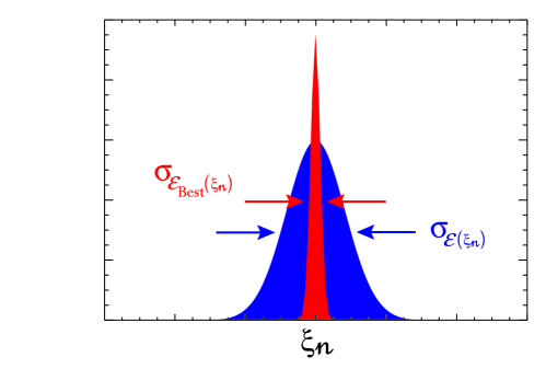
Figure 1.— Sketch comparing the variances of an arbitrary estimator of $\xi_{n}$ with the best estimator of the same quantity. The widest distribution does not permit an accurate determination of $\xi_{n}$ due to its large variance whilst the narrow distribution corresponds to the best (unbiased) estimator and possesses the smallest possible variance. As a consequence, one given realization (i.e. our CMB sky) will most probably be closest to the mean value in the second case rather than in the first one.

All the above analysis performed for the best (quantum) estimators can equally well be reproduced in the case where the anisotropies are due to an underlying stochastic process although the former is generally physically best motivated. In that case, quantum averages $\langle\Psi|\cdots|\Psi\rangle$ are just replaced with stochastic averages $\langle\cdots\rangle$. In the following, we will drop out the ‘hat’ symbol and consider that the different quantities are either operators or stochastic processes. In the same manner, we will denote an ensemble average by the symbol $\langle\cdots\rangle$ having in mind that this means either quantum or classical averages.

Let us now describe the relevant quantities to estimate. It is convenient to expand the temperature fluctuations over the basis of spherical harmonics according to

$$\Delta({\bf e})=\sum_{\ell m}a_{\ell}^{m}Y_{\ell}^{m}({\bf e}).$$ (6)

This equation assumes a complete sky coverage. Implementation of the method for the incomplete (galaxy-cut) sky can be performed by using the basis introduced in (Górski (1994)). Once a specific model is given, the statistical properties of the $a_{\ell}^{m}$’s are determined. Since $\Delta({\bf e})$ is real, the $a_{\ell}^{m}$’s must satisfy $a_{\ell}^{m*}=(-1)^{m}a_{\ell}^{-m}$. Without restricting the generality of the underlying physics, the first three moments can be written as

$$\bigl{\langle}a_{\ell}^{m}\bigr{\rangle}=0,\quad\bigl{\langle}a_{\ell_{1}}^{m_{1}}a_{\ell_{2}}^{m_{2}*}\bigr{\rangle}={\cal C}_{\ell_{1}}\delta_{\ell_{1}\ell_{2}}\delta_{m_{1}m_{2}},\quad\bigl{\langle}a_{\ell_{1}}^{m_{1}}a_{\ell_{2}}^{m_{2}}a_{\ell_{3}}^{m_{3}}\bigr{\rangle}=\left({}^{\ell_{1}~{}\,\;\ell_{2}~{}\,\;\ell_{3}}_{m_{1}~{}m_{2}~{}m_{3}}\right){\cal C}_{\ell_{1}\ell_{2}\ell_{3}},$$ (7)

where $\left({}^{\ell_{1}~{}\,\;\ell_{2}~{}\,\;\ell_{3}}_{m_{1}~{}m_{2}~{}m_{3}}\right)$ is a Wigner 3$j$-symbol. The second equation ensures the isotropy of the CMB. The quantity $\bigl{\langle}a_{\ell_{1}}^{m_{1}}a_{\ell_{2}}^{m_{2}*}\bigr{\rangle}$ is the second moment of the $a_{\ell}^{m}$’s and ${\cal C}_{\ell}$ is usually called the angular spectrum. In the third equation, the quantity $\bigl{\langle}a_{\ell_{1}}^{m_{1}}a_{\ell_{2}}^{m_{2}}a_{\ell_{3}}^{m_{3}}\bigr{\rangle}$ is the third moment while ${\cal C}_{\ell_{1}\ell_{2}\ell_{3}}$ is called the angular bispectrum. For $\ell_{1}=\ell_{2}=\ell_{3}=\ell$, this quantity is generally written as ${\cal B}_{\ell}\equiv{\cal C}_{\ell\ell\ell}$. The presence of the Wigner 3$j$-symbol guarantees that the third moment vanishes unless $m_{1}+m_{2}+m_{3}=0$ and $|\ell_{i}-\ell_{j}|\leq\ell_{k}\leq\ell_{i}+\ell_{j}$. Moreover, invariance under spatial inversions of $\xi_{3}$ implies an additional ‘selection rule’ (Luo (1994); Gangui & Martin (2000)), $\ell_{1}+\ell_{2}+\ell_{3}=\mbox{even}$, in order for the third moment not to vanish. Finally, from this last relation and using standard properties of the 3$j$-symbols, it follows that the angular bispectrum is left unchanged under any arbitrary permutation of the indices $\ell_{i}$.

We will need the higher moments as well. Since departures from Gaussianity are expected to be small (specially on large angular scales), higher moments will be calculated in the mildly non-Gaussian approximation. Within this approximation we can write $a_{\ell}^{m}=a_{\ell}^{m(0)}+\epsilon\,a_{\ell}^{m(1)}+{\cal O}(\epsilon^{2})$ where $a_{\ell}^{m(0)}$ is a Gaussian random variable and the expansion parameter $\epsilon$ is small. In the following, each moment will be calculated to the first non-vanishing order in $\epsilon$. For example, the fourth moment yields $\bigl{\langle}a_{\ell_{1}}^{m_{1}}a_{\ell_{2}}^{m_{2}}a_{\ell_{3}}^{m_{3}}a_{\ell_{4}}^{m_{4}}\bigr{\rangle}=\bigl{\langle}a_{\ell_{1}}^{m_{1}(0)}a_{\ell_{2}}^{m_{2}(0)}a_{\ell_{3}}^{m_{3}(0)}a_{\ell_{4}}^{m_{4}(0)}\bigr{\rangle}+{\cal O}(\epsilon)$. As a consequence, the connected fourth moment can be neglected because it is of higher order than the Gaussian part. The ‘⁽⁰⁾’ label will be dropped out hereafter. Therefore, in the mildly non-Gaussian approximation we can write

$$\bigl{\langle}a_{\ell_{1}}^{m_{1}}a_{\ell_{2}}^{m_{2}}a_{\ell_{3}}^{m_{3}*}a_{\ell_{4}}^{m_{4}*}\bigr{\rangle} \approx \bigl{\langle}a_{\ell_{1}}^{m_{1}}a_{\ell_{2}}^{m_{2}}\bigr{\rangle}\bigl{\langle}a_{\ell_{3}}^{m_{3}*}a_{\ell_{4}}^{m_{4}*}\bigr{\rangle}+\bigl{\langle}a_{\ell_{1}}^{m_{1}}a_{\ell_{3}}^{m_{3}*}\bigr{\rangle}\bigl{\langle}a_{\ell_{2}}^{m_{2}}a_{\ell_{4}}^{m_{4}*}\bigr{\rangle}+\bigl{\langle}a_{\ell_{1}}^{m_{1}}a_{\ell_{4}}^{m_{4}*}\bigr{\rangle}\bigl{\langle}a_{\ell_{2}}^{m_{2}}a_{\ell_{3}}^{m_{3}*}\bigr{\rangle}$$ (8)

$$= (-1)^{m_{2}+m_{4}}{\cal C}_{\ell_{1}}{\cal C}_{\ell_{3}}\delta_{\ell_{1}\ell_{2}}\delta_{m_{1},-m_{2}}\delta_{\ell_{3}\ell_{4}}\delta_{m_{3},-m_{4}}+{\cal C}_{\ell_{1}}{\cal C}_{\ell_{2}}\delta_{\ell_{1}\ell_{3}}\delta_{m_{1}m_{3}}\delta_{\ell_{2}\ell_{4}}\delta_{m_{2}m_{4}}$$

$$+ {\cal C}_{\ell_{1}}{\cal C}_{\ell_{2}}\delta_{\ell_{1}\ell_{4}}\delta_{m_{1}m_{4}}\delta_{\ell_{2}\ell_{3}}\delta_{m_{2}m_{3}}.$$

The fifth moment could be determined in a similar way but we will not need this quantity in the following. Finally, the sixth moment can be expressed as

$$\bigl{\langle}a_{\ell_{1}}^{m_{1}}a_{\ell_{2}}^{m_{2}}a_{\ell_{3}}^{m_{3}}a_{\ell_{4}}^{m_{4}*}a_{\ell_{5}}^{m_{5}*}a_{\ell_{6}}^{m_{6}*}\bigr{\rangle}\approx\bigl{\langle}a_{\ell_{1}}^{m_{1}}a_{\ell_{2}}^{m_{2}}\bigr{\rangle}\bigl{\langle}a_{\ell_{3}}^{m_{3}}a_{\ell_{4}}^{m_{4}*}\bigr{\rangle}\bigl{\langle}a_{\ell_{5}}^{m_{5}*}a_{\ell_{6}}^{m_{6}*}\bigr{\rangle}+\mbox{ 14 additional permutations }.$$ (9)

Although the explicit expression is not particularly illuminating, the last equation will be useful for the calculation of the variance when dealing with the three-point correlators below. In particular, one can write

$$\bigl{\langle}a_{\ell_{1}}^{m_{1}}a_{\ell_{2}}^{m_{2}}a_{\ell_{3}}^{m_{3}}a_{\ell_{1}}^{m_{1}*}a_{\ell_{2}}^{m_{2}*}a_{\ell_{3}}^{m_{3}*}\bigr{\rangle} = {\cal C}_{\ell_{1}}{\cal C}_{\ell_{2}}{\cal C}_{\ell_{3}}+2{\cal C}_{\ell_{1}}^{3}\delta_{\ell_{1}\ell_{2}\ell_{3}}(\delta_{m_{1}m_{3}}+\delta_{m_{1}-m_{3}})(\delta_{m_{1}m_{2}}+\delta_{m_{1}-m_{2}})$$ (10)

$$+ {\cal C}_{\ell_{1}}{\cal C}_{\ell_{2}}^{2}\delta_{\ell_{2}\ell_{3}}(\delta_{m_{2}m_{3}}+\delta_{m_{2}-m_{3}})+{\cal C}_{\ell_{2}}{\cal C}_{\ell_{3}}^{2}\delta_{\ell_{3}\ell_{1}}(\delta_{m_{1}m_{3}}+\delta_{m_{1}-m_{3}})$$

$$+ {\cal C}_{\ell_{3}}{\cal C}_{\ell_{1}}^{2}\delta_{\ell_{1}\ell_{2}}(\delta_{m_{1}m_{2}}+\delta_{m_{1}-m_{2}}),$$

where the symbol $\delta_{\ell_{1}\ell_{2}\ell_{3}}$ vanishes unless $\ell_{1}=\ell_{2}=\ell_{3}$ in which case it is one. This equation coincides with Eq. (24) of (Luo (1994)) provided the undefined symbol $\delta_{m_{1}m_{2}m_{3},0}$ written in that work has the meaning $\delta_{m_{1}m_{2}m_{3},0}\equiv(\delta_{m_{1}m_{3}}+\delta_{m_{1}-m_{3}})(\delta_{m_{1}m_{2}}+\delta_{m_{1}-m_{2}})$.

As we mentioned in the Introduction, in this article we are mainly interested in finding the best unbiased estimators for the two following quantities: the third moment $\bigl{\langle}a_{\ell_{1}}^{m_{1}}a_{\ell_{2}}^{m_{2}}a_{\ell_{3}}^{m_{3}}\bigr{\rangle}$ and the angular bispectrum ${\cal C}_{\ell_{1}\ell_{2}\ell_{3}}$. These are related to the three-point correlation function $\xi_{3}$. It is clear that, as mentioned above, the very same method could also be utilized for the computation of $\xi_{n}$ with $n$ arbitrary. Before addressing this question, however, we will first treat the analogous quantities related to the two-point correlation function, namely $\bigl{\langle}a_{\ell_{1}}^{m_{1}}a_{\ell_{2}}^{m_{2}*}\bigr{\rangle}$ and ${\cal C}_{\ell}$, the main purpose being to illustrate concretely the tactics presented above in a case where everything can be calculated easily. This will be used as a guideline for the case of the three-point correlators.

3. Two-point correlators

3.1. Best estimator for the angular spectrum ${\cal C}_{\ell}$

The definition of the estimator ${\cal E}({\cal C}_{\ell})$ is given by our general prescription, see Eq. (2)

$${\cal E}({\cal C}_{\ell})\equiv\int\int{\rm d}\Omega_{1}{\rm d}\Omega_{2}E^{\ell}({\bf e}_{1},{\bf e}_{2})\Delta({\bf e}_{1})\Delta({\bf e}_{2}),$$ (11)

where $E^{\ell}({\bf e}_{1},{\bf e}_{2})$ is the weight function. The angular spectrum ${\cal C}_{\ell}$ is a real quantity and its estimator ${\cal E}({\cal C}_{\ell})$ must also be real. Therefore, the weight function can be taken real. From the previous definition, it is clear that the antisymmetric part of $E^{\ell}({\bf e}_{1},{\bf e}_{2})$ does not contribute to the estimator. Then, we can replace $E^{\ell}({\bf e}_{1},{\bf e}_{2})$ in ${\cal E}({\cal C}_{\ell})$ by its symmetrized expression $E_{\rm S}^{\ell}({\bf e}_{1},{\bf e}_{2})=(1/2)[E^{\ell}({\bf e}_{1},{\bf e}_{2})+E^{\ell}({\bf e}_{2},{\bf e}_{1})]$. At this stage, two methods can be applied. Either we work directly with the weight function or we expand it over the spherical harmonics basis and try to determine the coefficients of this expansion. Clearly, both paths are equivalent and can be followed for any estimator. Here we employ the second method, leaving the first one for the determination of the second-moment estimator considered in the next subsection. Therefore, we write the weight function as

$$E^{\ell}_{\rm S}({\bf e}_{1},{\bf e}_{2})=\sum_{\ell_{1}m_{1}}\sum_{\ell_{2}m_{2}}{\rm d}^{\ \ell}_{\left\{\!\!\tiny\begin{array}[]{ccc}\!\ell_{1}\!\!&\!\!\ell_{2}\!\\ \!m_{1}\!\!&\!\!m_{2}\!\end{array}\!\!\right\}}Y_{\ell_{1}}^{m_{1}}({\bf e}_{1})Y_{\ell_{2}}^{m_{2}}({\bf e}_{2}).$$ (12)

The reality and symmetry properties of the weight function $E_{\rm S}^{\ell}$ imply that the complex coefficient of the expansion must satisfy, respectively

$${\rm d}^{\ \ell*}_{\left\{\!\!\tiny\begin{array}[]{ccc}\!\ell_{1}\!\!&\!\!\ell_{2}\!\\ \!m_{1}\!\!&\!\!m_{2}\!\end{array}\!\!\right\}}=(-1)^{m_{1}+m_{2}}{\rm d}^{\ \ell}_{\left\{\!\!\tiny\begin{array}[]{ccc}\!\ell_{1}\!\!&\!\!\ell_{2}\!\\ \!-m_{1}\!\!&\!\!-m_{2}\!\end{array}\!\!\right\}}\quad,\quad{\rm d}^{\ \ell}_{\left\{\!\!\tiny\begin{array}[]{ccc}\!\ell_{1}\!\!&\!\!\ell_{2}\!\\ \!m_{1}\!\!&\!\!m_{2}\!\end{array}\!\!\right\}}={\rm d}^{\ \ell}_{\left\{\!\!\tiny\begin{array}[]{ccc}\!\ell_{2}\!\!&\!\!\ell_{1}\!\\ \!m_{2}\!\!&\!\!m_{1}\!\end{array}\!\!\right\}}.$$ (13)

Inserting the expression of the weight function (12) into the general definition of the estimator (11) and using standard properties of the spherical harmonics, one gets

$${\cal E}({\cal C}_{\ell})=\sum_{\ell_{1}m_{1}}\sum_{\ell_{2}m_{2}}{\rm d}^{\ \ell*}_{\left\{\!\!\tiny\begin{array}[]{ccc}\!\ell_{1}\!\!&\!\!\ell_{2}\!\\ \!m_{1}\!\!&\!\!m_{2}\!\end{array}\!\!\right\}}a_{\ell_{1}}^{m_{1}}a_{\ell_{2}}^{m_{2}}.$$ (14)

Our first move is now to require that $\langle{\cal E}({\cal C}_{\ell})\rangle={\cal C}_{\ell}$. Using the second of Eqns. (7), we find that the coefficients $d$ must fulfill the following constraints

$$\sum_{m_{1}}(-1)^{m_{1}}{\rm d}^{\ \ell}_{\left\{\!\!\tiny\begin{array}[]{ccc}\!\ell_{1}\!\!&\!\!\ell_{1}\!\\ \!-m_{1}\!\!&\!\!m_{1}\!\end{array}\!\!\right\}}=\delta^{\ell}_{\ell_{1}}.$$ (15)

All the estimators satisfying this condition are unbiased. However, it is clear that this does not completely determines the estimator but just a class of estimators. Our second move is to calculate the variance. Using Eq. (8), a straightforward computation gives

$$\sigma^{2}_{{\cal E}({\cal C}_{\ell})}=2\sum_{\ell_{1}m_{1}}\sum_{\ell_{2}m_{2}}{\rm d}^{\ \ell*}_{\left\{\!\!\tiny\begin{array}[]{ccc}\!\ell_{1}\!\!&\!\!\ell_{2}\!\\ \!m_{1}\!\!&\!\!m_{2}\!\end{array}\!\!\right\}}{\rm d}^{\ \ell}_{\left\{\!\!\tiny\begin{array}[]{ccc}\!\ell_{1}\!\!&\!\!\ell_{2}\!\\ \!m_{1}\!\!&\!\!m_{2}\!\end{array}\!\!\right\}}{\cal C}_{\ell_{1}}{\cal C}_{\ell_{2}}.$$ (16)

This quantity is obviously positive. From this expression, one sees that the imaginary part of the coefficients $d$ only increases the variance. Since a vanishing $\Im({\rm d})$ satisfies the constraint equation, we can consider that the $d$’s are real.

Our third move is to minimize the variance taking into account the constraint. For this purpose we introduce a set of Lagrange multipliers $\lambda^{\ell}_{\ell_{1}}$ (i.e. one Lagrange multiplier per constraint since $\ell$ must be seen as a fixed index) and require that

$$\delta\biggl{[}\sigma^{2}_{{\cal E}({\cal C}_{\ell})}+\sum_{\ell_{1}}\lambda^{\ell}_{\ell_{1}}\biggl{(}\sum_{m_{1}}(-1)^{m_{1}}{\rm d}^{\ \ell}_{\left\{\!\!\tiny\begin{array}[]{ccc}\!\ell_{1}\!\!&\!\!\ell_{1}\!\\ \!-m_{1}\!\!&\!\!m_{1}\!\end{array}\!\!\right\}}-\delta^{\ell}_{\ell_{1}}\biggl{)}\biggr{]}=0.$$ (17)

The definition of the variation $\delta$ must respect the symmetry properties of the coefficients $d$; we take

$${\delta{\rm d}^{\ \ell}_{\left\{\!\!\tiny\begin{array}[]{ccc}\!\ \ell_{1}\ \!\!&\!\!\ \ell_{2}\ \!\\ \!\ m_{1}\ \!\!&\!\!\ m_{2}\ \!\end{array}\!\!\right\}}\over\delta{\rm d}^{\ \ell}_{\left\{\!\!\tiny\begin{array}[]{ccc}\!\ \ell_{1}^{\prime}\ \!\!&\!\!\ \ell_{2}^{\prime}\ \!\\ \!\ m_{1}^{\prime}\ \!\!&\!\!\ m_{2}^{\prime}\ \!\end{array}\!\!\right\}}}\equiv\frac{1}{2} \biggl{\{} \frac{1}{2}\delta_{\ell_{1}\ell_{1}^{\prime}}\delta_{\ell_{2}\ell_{2}^{\prime}}\biggl{[}\delta_{m_{1}m_{1}^{\prime}}\delta_{m_{2}m_{2}^{\prime}}+(-1)^{m_{1}+m_{2}}\delta_{m_{1}-m_{1}^{\prime}}\delta_{m_{2}-m_{2}^{\prime}}\biggr{]}$$ (22)

$$+ \frac{1}{2}\delta_{\ell_{1}\ell_{2}^{\prime}}\delta_{\ell_{2}\ell_{1}^{\prime}}\biggl{[}\delta_{m_{1}m_{2}^{\prime}}\delta_{m_{2}m_{1}^{\prime}}+(-1)^{m_{1}+m_{2}}\delta_{m_{1}-m_{2}^{\prime}}\delta_{m_{2}-m_{1}^{\prime}}\biggr{]}\biggr{\}}.$$ (23)

Although it is not compulsory to use this equation, since a naive definition of the variation would lead to the same final result (Grishchuk & Martin (1997)), it is nevertheless interesting to utilize it as a warm up for what will be done for the angular bispectrum. The variation leads to the following relation between the coefficients $d$ and the Lagrange multipliers

$$4{\rm d}^{\ \ell}_{\left\{\!\!\tiny\begin{array}[]{ccc}\!\ell_{1}\!\!&\!\!\ell_{2}\!\\ \!m_{1}\!\!&\!\!m_{2}\!\end{array}\!\!\right\}}{\cal C}_{\ell_{1}}{\cal C}_{\ell_{2}}+(-1)^{m_{1}}\lambda^{\ell}_{\ell_{1}}\delta_{\ell_{1}\ell_{2}}\delta_{m_{1}-m_{2}}=0.$$ (24)

We see that the choice of the $\lambda^{\ell}$’s is not free; it is fixed by the variation itself. Using the constraint in this equation, we find $\lambda^{\ell}_{\ell_{1}}=-4[{\cal C}_{\ell_{1}}^{2}/(2\ell_{1}+1)]\delta^{\ell}_{\ell_{1}}$. Having determined what the Lagrange multipliers are, the problem is completely solved. It is now sufficient to re-introduce this value for $\lambda^{\ell}_{\ell_{1}}$ in Eq. (24), get the coefficients $d$ and, from this, also the best unbiased estimator: the weight function is then given by $E_{\rm S,Best}^{\ell}({\bf e}_{1},{\bf e}_{2})=(1/4\pi)P_{\ell}({\bf e}_{1}\cdot{\bf e}_{2})$ and the estimator itself by (see also Grishchuk & Martin (1997))

$${\cal E}_{\rm Best}({\cal C}_{\ell})=\frac{1}{2\ell+1}\sum_{m=-\ell}^{\ell}a_{\ell}^{m}a_{\ell}^{m*}.$$ (25)

The variance of this estimator is the well-known ‘cosmic variance’

$$\sigma^{2}_{{\cal E}_{\rm Best}({\cal C}_{\ell})}=\frac{2{\cal C}_{\ell}^{2}}{2\ell+1}.$$ (26)

One remark is in order here. The cosmic variance is usually obtained in the following way: the previous estimator appears naturally from Eqns. (7) and it is usually assumed that the $a_{\ell}^{m}$’s are Gaussian random variables. In this case, the estimator (25) has a $\chi^{2}$ probability density function and from this the cosmic variance can be easily recovered. The proof presented above is by no means equivalent to this naive derivation. There are many unbiased estimators and, a priori, nothing guarantees that the simplest one is the best one, i.e. the naive derivation is not sufficient to prove that the estimator (25) is the best one. This can be proven only along the lines described above. Moreover, we do not need to assume that the $a_{\ell}^{m}$’s obey a Gaussian statistics. Only the mildly non-Gaussian assumption is necessary for the calculation of the four-point correlators.

3.2. Best estimator for the second moment ${\cal C}_{\alpha}$

In this section, we discuss the best estimator for ${\cal C}_{\alpha}\equiv\bigl{\langle}a_{\ell_{1}}^{m_{1}}a_{\ell_{2}}^{m_{2}*}\bigr{\rangle}$. Greek letters will always be employed for collective-index notation, like $\alpha\equiv{\left\{\!\!\tiny\begin{array}[]{cc}\!\ell_{1}\!\!&\!\!\ell_{2}\!\\ \!m_{1}\!\!&\!\!m_{2}\!\end{array}\!\!\right\}}$ or $\alpha^{\prime}\equiv{\left\{\!\!\tiny\begin{array}[]{cc}\!\ell_{1}^{\prime}\!\!&\!\!\ell_{2}^{\prime}\!\\ \!m_{1}^{\prime}\!\!&\!\!m_{2}^{\prime}\!\end{array}\!\!\right\}}$. Unlike in the foregoing subsection, we find the weight function directly without expanding it over the spherical harmonics basis. This method is closer to the one used by Heavens (1998). We also show that the best estimator of ${\cal C}_{\alpha}$ cannot be deduced from the best estimator of the angular spectrum ${\cal C}_{\ell}$ obtained in the previous subsection as one could naively think.

Let us start with a couple of definitions. First, the quantity

$$R^{\alpha}({\bf e}_{1},{\bf e}_{2})\equiv Y_{\ell_{1}}^{m_{1}}({\bf e}_{1})Y_{\ell_{2}}^{m_{2}*}({\bf e}_{2}),$$ (27)

which is complex and non-symmetric with regards to the position of the complex conjugate symbol ‘^∗’. This last property comes from the definition of $\bigl{\langle}a_{\ell_{1}}^{m_{1}}a_{\ell_{2}}^{m_{2}*}\bigr{\rangle}$ itself and it would be the case for any even-point correlator. Then, regarding complex conjugation, there is a slight difference between the even- and the odd-point correlators. The real part of $R^{\alpha}({\bf e}_{1},{\bf e}_{2})$ will be noted

$$R^{\alpha}_{\rm R}({\bf e}_{1},{\bf e}_{2})\equiv\frac{1}{2}\biggl{[}Y_{\ell_{1}}^{m_{1}}({\bf e}_{1})Y_{\ell_{2}}^{m_{2}*}({\bf e}_{2})+Y_{\ell_{1}}^{m_{1}*}({\bf e}_{1})Y_{\ell_{2}}^{m_{2}}({\bf e}_{2})\biggr{]}.$$ (28)

$R^{\alpha}_{\rm R}({\bf e}_{1},{\bf e}_{2})$ is not symmetric under a permutation of the two directions. It satisfies $R^{\alpha}_{\rm R}({\bf e}_{2},{\bf e}_{1})=R^{\bar{\alpha}}_{\rm R}({\bf e}_{1},{\bf e}_{2})$, where the index $\bar{\alpha}$ is defined by $\bar{\alpha}\equiv{\tiny\{\begin{array}[]{ccc}\!\ell_{2}\!&\!\ell_{1}\!\\ \!m_{2}\!&\!m_{1}\!\end{array}\}}$. The symmetries in the indices and in the directions will play an important rôle in what follows. Using the previous definitions, we can introduce a quantity which is symmetric both under a permutation of the two directions and under a permutation of the columns of internal indices in $\alpha$

$$R^{\alpha}_{\rm S}({\bf e}_{1},{\bf e}_{2})\equiv\frac{1}{4}\biggl{[}Y_{\ell_{1}}^{m_{1}}({\bf e}_{1})Y_{\ell_{2}}^{m_{2}*}({\bf e}_{2})+Y_{\ell_{1}}^{m_{1}}({\bf e}_{2})Y_{\ell_{2}}^{m_{2}*}({\bf e}_{1})+Y_{\ell_{1}}^{m_{1}*}({\bf e}_{1})Y_{\ell_{2}}^{m_{2}}({\bf e}_{2})+Y_{\ell_{1}}^{m_{1}*}({\bf e}_{2})Y_{\ell_{2}}^{m_{2}}({\bf e}_{1})\biggr{]},$$ (29)

i.e. we have $R^{\alpha}_{\rm S}({\bf e}_{1},{\bf e}_{2})=R^{\alpha}_{\rm S}({\bf e}_{2},{\bf e}_{1})=R^{\bar{\alpha}}_{\rm S}({\bf e}_{1},{\bf e}_{2})=R^{\bar{\alpha}}_{\rm S}({\bf e}_{2},{\bf e}_{1})$. Finally, we will also employ a symmetrized Krönecker symbol defined according to

$$\delta^{\alpha\alpha^{\prime}}_{\rm S}\equiv\frac{1}{2}\biggl{(}\delta_{\ell_{1}\ell_{1}^{\prime}}\delta_{\ell_{2}\ell_{2}^{\prime}}\delta_{m_{1}m_{1}^{\prime}}\delta_{m_{2}m_{2}^{\prime}}+\delta_{\ell_{1}\ell_{2}^{\prime}}\delta_{\ell_{2}\ell_{1}^{\prime}}\delta_{m_{1}m_{2}^{\prime}}\delta_{m_{2}m_{1}^{\prime}}\biggr{)},$$ (30)

which is left unchanged under a permutation of the indices $\alpha$ and $\alpha^{\prime}$ and also under permutations of the columns of each collective index separately.

Let us now turn to the computation of the best unbiased estimator; the general definition of an estimator can be expressed as

$${\cal E}({\cal C}_{\alpha})\equiv\int\int{\rm d}\Omega_{1}{\rm d}\Omega_{2}E^{\alpha}({\bf e}_{1},{\bf e}_{2})\Delta({\bf e}_{1})\Delta({\bf e}_{2}).$$ (31)

The quantity ${\cal C}_{\alpha}$ is unchanged if we permute the columns of indices in $\alpha$, ${\cal C}_{\alpha}={\cal C}_{\bar{\alpha}}$ with $\bar{\alpha}$ given above. Being an estimator for ${\cal C}_{\alpha}$ it is then natural to assume that ${\cal E}({\cal C}_{\alpha})$ possesses the same property, ${\cal E}({\cal C}_{\alpha})={\cal E}({\cal C}_{\bar{\alpha}})$. Looking at the definition of $E^{\alpha}({\bf e}_{1},{\bf e}_{2})$, Eq. (31), we easily see that the weight function will also satisfy $E^{\alpha}({\bf e}_{1},{\bf e}_{2})=E^{\bar{\alpha}}({\bf e}_{1},{\bf e}_{2})$. Moreover, we take $E^{\alpha}({\bf e}_{1},{\bf e}_{2})$ symmetric under a permutation in the directions ${\bf e}_{1}$ and ${\bf e}_{2}$, i.e. $E_{\rm S}^{\alpha}({\bf e}_{1},{\bf e}_{2})=E_{\rm S}^{\alpha}({\bf e}_{2},{\bf e}_{1})$.

Now, we require that the estimator ${\cal E}(C_{\alpha})$ be unbiased, which implies that the following relation must be fulfilled

$$\int\int{\rm d}\Omega_{1}{\rm d}\Omega_{2}E_{\rm S}^{\alpha}({\bf e}_{1},{\bf e}_{2})R^{\alpha^{\prime}}({\bf e}_{1},{\bf e}_{2})=\delta^{\alpha\alpha^{\prime}}_{\rm S}.$$ (32)

We have required the presence of $\delta^{\alpha\alpha^{\prime}}_{\rm S}$ in the right hand side of the previous equation to respect the symmetries in $\alpha$ of the weight function. In the previous equation the $E_{\rm S}^{\alpha}$ and $R^{\alpha^{\prime}}$ are a priori complex. However, one can show that it is possible to work only with a real weight function, $E_{\rm S}^{{\alpha}*}({\bf e}_{1},{\bf e}_{2})=E_{\rm S}^{\alpha}({\bf e}_{1},{\bf e}_{2})$ and with the $R^{\alpha}_{\rm R}({\bf e}_{1},{\bf e}_{2})$ defined above: the imaginary contributions would just increase the variance. (One could have also chosen to work with a pure imaginary weight function and the imaginary part of $R^{\alpha}$). Therefore, the constraint can be written as

$$\int\int{\rm d}\Omega_{1}{\rm d}\Omega_{2}E_{\rm S}^{\alpha}({\bf e}_{1},{\bf e}_{2})R_{\rm R}^{\alpha^{\prime}}({\bf e}_{1},{\bf e}_{2})=\delta^{\alpha\alpha^{\prime}}_{\rm S},$$ (33)

where $E_{\rm S}^{\alpha}$ has been taken real. Let us now calculate the variance of the estimator ${\cal E}({\cal C}_{\alpha})$. Using Eqns. (8), we easily find that

$$\sigma^{2}_{{\cal E}({\cal C}_{\alpha})}=2\int\int\int\int{\rm d}\Omega_{1}{\rm d}\Omega_{2}{\rm d}\Omega_{3}{\rm d}\Omega_{4}E_{\rm S}^{\alpha}({\bf e}_{1},{\bf e}_{2})E_{\rm S}^{\alpha}({\bf e}_{3},{\bf e}_{4})\xi({\bf e}_{1}\!\cdot\!{\bf e}_{3})\xi({\bf e}_{2}\!\cdot\!{\bf e}_{4}).$$ (34)

Our next step is to minimize this variance under the constraint given in Eq. (33). For this purpose, we introduce a set of Lagrange multipliers $\lambda^{\alpha}$ and require that

$$\delta\biggr{[}\sigma^{2}_{{\cal E}({\cal C}_{\alpha})}+\sum_{\alpha^{\prime}}\lambda^{\alpha}_{\alpha^{\prime}}\biggl{(}\int\int{\rm d}\Omega_{1}{\rm d}\Omega_{2}E_{\rm S}^{\alpha}({\bf e}_{1},{\bf e}_{2})R^{\alpha^{\prime}}_{\rm R}({\bf e}_{1},{\bf e}_{2})-\delta^{\alpha\alpha^{\prime}}_{\rm S}\biggr{)}\biggr{]}=0.$$ (35)

At this point the precise meaning of the variation symbol $\delta$ matters. Before performing the variation, let us recall that the symmetries of the weight function must be respected; hence we will have

$$\frac{{\rm\delta}E_{\rm S}^{\alpha}({\bf e}_{i},{\bf e}_{j})}{{\rm\delta}E_{\rm S}^{\beta}({\bf e}_{k},{\bf e}_{\ell})}=\frac{1}{2}\biggl{[}{\delta({\bf e}_{i}\!\cdot\!{\bf e}_{k}-1)\over 2\pi}{\delta({\bf e}_{j}\!\cdot\!{\bf e}_{\ell}-1)\over 2\pi}+{\delta({\bf e}_{i}\!\cdot\!{\bf e}_{\ell}-1)\over 2\pi}{\delta({\bf e}_{j}\!\cdot\!{\bf e}_{k}-1)\over 2\pi}\biggr{]}\delta^{\alpha\beta}_{\rm S}.$$ (36)

The $2\pi$’s in the denominators come from the fact that, while the direction ${\bf e}_{i}$ is expressed in terms of the corresponding spherical angles like ${\bf e}_{i}\equiv(\theta_{i},\varphi_{i})$ and then ${\rm d}\Omega_{i}={\rm d}\cos\theta_{i}{\rm d}\varphi_{i}$, there is an extra $2\pi$ factor in $\delta({\bf e}_{i}\!\cdot\!{\bf e}_{k}-1)=2\pi\,\delta(\cos\theta_{i}-\cos\theta_{k})\delta(\varphi_{i}-\varphi_{k})$. As a result of the variation, we obtain the following equation

$$\int\int{\rm d}\Omega_{1}{\rm d}\Omega_{2}E_{\rm S}^{\alpha}({\bf e}_{1},{\bf e}_{2})\xi({\bf e}_{1}\!\cdot\!{\bf e}_{3})\xi({\bf e}_{2}\!\cdot\!{\bf e}_{4})=\frac{1}{4}\sum_{\alpha^{\prime}}\lambda^{\alpha}_{\alpha^{\prime}}R_{\rm S}^{\alpha^{\prime}}({\bf e}_{3},{\bf e}_{4}).$$ (37)

The quantity $R_{\rm S}^{\alpha^{\prime}}({\bf e}_{3},{\bf e}_{4})$ appears naturally as a result of Eq. (36). The previous equation should be compared with Eq. (24) of the previous subsection. The result of the variation is a relation between the weight function and the Lagrange multiplier. Our aim now is to get an explicit expression for the weight function. This can be done by using the inverse two-point correlation function $\xi^{-1}$ which satisfies (see also the Appendix)

$$\int{\rm d}\Omega_{j}\xi({\bf e}_{i}\!\cdot\!{\bf e}_{j})\xi^{-1}({\bf e}_{j}\!\cdot\!{\bf e}_{k})\equiv\delta({\bf e}_{i}\!\cdot\!{\bf e}_{k}-1).$$ (38)

In the case of the three-point correlator, this definition leads to subtleties which will be examined in detail in the next section. Multiplying Eq. (37) by $\xi^{-1}({\bf e}_{1^{\prime}}\cdot{\bf e}_{3})\xi^{-1}({\bf e}_{2^{\prime}}\cdot{\bf e}_{4})$, integrating over directions ${\bf e}_{3}$ and ${\bf e}_{4}$ and relabelling indices, we arrive at

$$E_{\rm S}^{\alpha}({\bf e}_{1},{\bf e}_{2})=\frac{1}{4}\frac{1}{(2\pi)^{2}}\sum_{\alpha^{\prime}}\int\int{\rm d}\Omega_{3}{\rm d}\Omega_{4}\lambda^{\alpha}_{\alpha^{\prime}}\xi^{-1}({\bf e}_{1}\!\cdot\!{\bf e}_{3})\xi^{-1}({\bf e}_{2}\!\cdot\!{\bf e}_{4})R_{\rm S}^{\alpha^{\prime}}({\bf e}_{3},{\bf e}_{4}).$$ (39)

This equation for the second moment is the analogous of Eq. (21) of (Heavens (1998)) obtained for the third moment. It is clear from the previous section that, at this stage, our final goal has not yet been reached. The weight function is still expressed in terms of the Lagrange multipliers. The correct way to proceed is to remove the latter using the constraint given by Eq. (33) as it was done in the previous subsection. Then, we first multiply Eq. (39) by the quantity $R_{\rm S}^{\alpha^{\prime\prime}}({\bf e}_{1},{\bf e}_{2})$ and, after having integrated over solid angles $\Omega_{1}$ and $\Omega_{2}$, this leads to the equation that the Lagrange multipliers must satisfy

$$16{\cal C}_{\ell_{1}^{\prime\prime}}{\cal C}_{\ell_{2}^{\prime\prime}}\delta^{\alpha\alpha^{\prime\prime}}_{\rm S}=\biggl{[}(-1)^{m_{1}^{\prime\prime}+m_{2}^{\prime\prime}}\lambda^{\alpha}_{\left\{\!\!\!\tiny\begin{array}[]{cc}\ell_{1}^{\prime\prime}\!&\!\ell_{2}^{\prime\prime}\\ -m_{1}^{\prime\prime}\!&\!-m_{2}^{\prime\prime}\end{array}\!\!\!\right\}}+(-1)^{m_{1}^{\prime\prime}+m_{2}^{\prime\prime}}\lambda^{\alpha}_{\left\{\!\!\!\tiny\begin{array}[]{cc}\ell_{2}^{\prime\prime}\!&\!\ell_{1}^{\prime\prime}\\ -m_{2}^{\prime\prime}\!&\!-m_{1}^{\prime\prime}\end{array}\!\!\!\right\}}+\lambda^{\alpha}_{\left\{\!\!\!\tiny\begin{array}[]{cc}\ell_{1}^{\prime\prime}\!&\!\ell_{2}^{\prime\prime}\\ m_{1}^{\prime\prime}\!&\!m_{2}^{\prime\prime}\end{array}\!\!\!\right\}}+\lambda^{\alpha}_{\left\{\!\!\!\tiny\begin{array}[]{cc}\ell_{2}^{\prime\prime}\!&\!\ell_{1}^{\prime\prime}\\ m_{2}^{\prime\prime}\!&\!m_{1}^{\prime\prime}\end{array}\!\!\!\right\}}\biggr{]}.$$ (40)

This equation is the analogue of the equation $\lambda^{\ell}_{\ell_{1}}=-4[{\cal C}_{\ell_{1}}^{2}/(2\ell_{1}+1)]\delta^{\ell}_{\ell_{1}}$ of the previous subsection. Here, the difference is that a combination of Lagrange multipliers with different indices appears rather than the Lagrange multiplier itself. However, we can reconstruct exactly this combination in the right hand side of Eq. (39). Indeed, we just have to multiply each side of Eq. (40) by $R_{\rm S}^{\alpha^{\prime\prime}}({\bf e}_{1},{\bf e}_{2})$ and perform the sum over $\alpha^{\prime\prime}$. Using the symmetry properties of $R_{\rm S}^{\alpha^{\prime\prime}}({\bf e}_{1},{\bf e}_{2})$ we obtain

$$4{\cal C}_{\ell_{1}}{\cal C}_{\ell_{2}}R_{\rm S}^{\alpha}({\bf e}_{1},{\bf e}_{2})=\sum_{\alpha^{\prime\prime}}\lambda^{\alpha}_{\alpha^{\prime\prime}}R_{\rm S}^{\alpha^{\prime\prime}}({\bf e}_{1},{\bf e}_{2}).$$ (41)

We now insert this equation in the right hand side of Eq. (39) to remove the Lagrange multipliers and find

$$E^{\alpha}_{\rm S,Best}({\bf e}_{1},{\bf e}_{2})=\frac{1}{4\pi^{2}}{\cal C}_{\ell_{1}}{\cal C}_{\ell_{2}}\int\int{\rm d}\Omega_{3}{\rm d}\Omega_{4}\xi^{-1}({\bf e}_{1}\!\cdot\!{\bf e}_{3})\xi^{-1}({\bf e}_{2}\!\cdot\!{\bf e}_{4})R_{\rm S}^{\alpha}({\bf e}_{3},{\bf e}_{4}).$$ (42)

To go further, we express $\xi^{-1}$ in Eq. (42) explicitly in terms of spherical harmonics (see the Appendix) which yields $E_{\rm S,Best}^{\alpha}({\bf e}_{1},{\bf e}_{2})=R_{\rm S}^{\alpha}({\bf e}_{1},{\bf e}_{2})$. Now, we just plug this result into Eq. (31) to get the final explicit expression of the best unbiased estimator ${\cal E}_{\rm Best}({\cal C}_{\alpha})$

$${\cal E}_{\rm Best}({\cal C}_{\alpha})=\frac{1}{2}\biggl{(}a_{\ell_{1}}^{m_{1}*}a_{\ell_{2}}^{m_{2}}+a_{\ell_{1}}^{m_{1}}a_{\ell_{2}}^{m_{2}*}\biggr{)}.$$ (43)

Some remarks are in order here. First, despite appearances, one cannot deduce ${\cal E}_{\rm Best}({\cal C}_{\alpha})$ from ${\cal E}_{\rm Best}({\cal C}_{\ell_{1}})$. It is clear that the following equation holds

$$\langle{\cal E}({\cal C}_{\alpha})\rangle=\langle{\cal E}({\cal C}_{\ell_{1}})\rangle\delta_{\ell_{1}\ell_{2}}\delta_{m_{1}m_{2}}.$$ (44)

However, from this equation we are not allowed to conclude that ${\cal E}_{\rm Best}({\cal C}_{\alpha})={\cal E}_{\rm Best}({\cal C}_{\ell_{1}})\delta_{\ell_{1}\ell_{2}}\delta_{m_{1}m_{2}}$. Therefore, knowing one of the best unbiased estimators does not allow us to infer the other best one. To be specific, if one assumed the previous wrong relation, from Eq. (25) one would get

$${\cal E}_{\rm Best}({\cal C}_{\alpha})=\frac{1}{2\ell_{1}+1}\biggl{(}\sum_{m=-\ell_{1}}^{\ell_{1}}a_{\ell_{1}}^{m*}a_{\ell_{1}}^{m}\biggr{)}\delta_{\ell_{1}\ell_{2}}\delta_{m_{1}m_{2}}\quad\mbox{(false)},$$ (45)

and although this estimator is unbiased, it is not the best one. The second remark is that although the estimator given by Eq. (43) could be naively regarded as a trivial one, this is not the case. Indeed, the estimator of Eq. (45) is as trivial as the actual best one. The moral is then that there exist simple choices which lead to the wrong answer. The only reliable method in the problem of minimizing the variance is therefore the one exposed above.

4. Three-point correlators

4.1. Best estimator for the angular bispectrum ${\cal C}_{\ell_{1}\ell_{2}\ell_{3}}$

In this section, our aim is to determine the best unbiased estimator for the angular bispectrum ${\cal C}_{\ell_{1}\ell_{2}\ell_{3}}$ defined in the third of Eqns. (7). According to our general prescription, the most general definition reads

$${\cal E}({\cal C}_{\ell_{1}\ell_{2}\ell_{3}})\equiv\int\int\int{\rm d}\Omega_{1}{\rm d}\Omega_{2}{\rm d}\Omega_{3}E_{\rm S}^{\ell_{1}\ell_{2}\ell_{3}}({\bf e}_{1},{\bf e}_{2},{\bf e}_{3})\Delta({\bf e}_{1})\Delta({\bf e}_{2})\Delta({\bf e}_{3}).$$ (46)

As in the case of the two-point correlators, the weight function also possesses the properties of being real and symmetric under arbitrary permutations of directions ${\bf e}_{i}$. In addition, like ${\cal C}_{\ell_{1}\ell_{2}\ell_{3}}$, the weight function satisfies $E_{\rm S}^{\ell_{1}\ell_{2}\ell_{3}}=E_{\rm S}^{\ell_{2}\ell_{1}\ell_{3}}$, as well as for any other arbitrary permutation of the indices $\ell_{i}$. We follow similar steps as for the angular spectrum and therefore we choose to expand the weight function on the basis of the spherical harmonics. Then, as in Eq. (12), we write

$$E_{\rm S}^{\ell_{1}\ell_{2}\ell_{3}}({\bf e}_{1},{\bf e}_{2},{\bf e}_{3})=\sum_{\ell_{1}^{\prime}m_{1}^{\prime}}\sum_{\ell_{2}^{\prime}m_{2}^{\prime}}\sum_{\ell_{3}^{\prime}m_{3}^{\prime}}{\rm d}^{\tiny\begin{array}[]{ccc}\!\ell_{1}\!&\!\ell_{2}\!&\ell_{3}\end{array}}_{\left\{\!\!\tiny\begin{array}[]{ccc}\!\ell_{1}^{\prime}\!\!&\!\!\ell_{2}^{\prime}\!\!&\!\!\ell_{3}^{\prime}\!\\ \!m_{1}^{\prime}\!\!&\!\!m_{2}^{\prime}\!\!&\!\!m_{3}^{\prime}\!\end{array}\!\!\right\}}Y_{\ell_{1}^{\prime}}^{m_{1}^{\prime}}({\bf e}_{1})Y_{\ell_{2}^{\prime}}^{m_{2}^{\prime}}({\bf e}_{2})Y_{\ell_{3}^{\prime}}^{m_{3}^{\prime}}({\bf e}_{3}).$$ (47)

The properties of the weight function imply that the coefficients $d$ must satisfy equations similar to those given in Eqns. (13)

$${\rm d}^{\tiny\begin{array}[]{ccc}\!\ell_{1}\!&\!\ell_{2}\!&\ell_{3}*\end{array}}_{\left\{\!\!\tiny\begin{array}[]{ccc}\!\ell_{1}^{\prime}\!\!&\!\!\ell_{2}^{\prime}\!\!&\!\!\ell_{3}^{\prime}\!\\ \!m_{1}^{\prime}\!\!&\!\!m_{2}^{\prime}\!\!&\!\!m_{3}^{\prime}\!\end{array}\!\!\right\}}=(-1)^{m_{1}^{\prime}+m_{2}^{\prime}+m_{3}^{\prime}}{\rm d}^{\tiny\begin{array}[]{ccc}\!\ell_{1}\!&\!\ell_{2}\!&\ell_{3}\end{array}}_{\left\{\!\!\tiny\begin{array}[]{ccc}\!\ell_{1}^{\prime}\!\!&\!\!\ell_{2}^{\prime}\!\!&\!\!\ell_{3}^{\prime}\!\\ \!-m_{1}^{\prime}\!\!&\!\!-m_{2}^{\prime}\!\!&\!\!-m_{3}^{\prime}\!\end{array}\!\!\right\}}\quad,\quad{\rm d}^{\tiny\begin{array}[]{ccc}\!\ell_{1}\!&\!\ell_{2}\!&\ell_{3}\end{array}}_{\left\{\!\!\tiny\begin{array}[]{ccc}\!\ell_{1}^{\prime}\!\!&\!\!\ell_{2}^{\prime}\!\!&\!\!\ell_{3}^{\prime}\!\\ \!m_{1}^{\prime}\!\!&\!\!m_{2}^{\prime}\!\!&\!\!m_{3}^{\prime}\!\end{array}\!\!\right\}}={\rm d}^{\tiny\begin{array}[]{ccc}\!\ell_{1}\!&\!\ell_{2}\!&\ell_{3}\end{array}}_{\left\{\!\!\tiny\begin{array}[]{ccc}\!\ell_{2}^{\prime}\!\!&\!\!\ell_{1}^{\prime}\!\!&\!\!\ell_{3}^{\prime}\!\\ \!m_{2}^{\prime}\!\!&\!\!m_{1}^{\prime}\!\!&\!\!m_{3}^{\prime}\!\end{array}\!\!\right\}},$$ (48)

where the last relation is in fact valid for arbitrary permutations of any two columns of the collective subindex. Like the weight function, $d$ is also left invariant under arbitrary permutations of indices $\ell_{i}$ (not primed). The estimator can be expressed in terms of the coefficients $d$ and the $a_{\ell}^{m}$’s only: inserting the expansion of the weight function in the above expression for the estimator and using standard properties of the spherical harmonics one obtains

$${\cal E}({\cal C}_{\ell_{1}\ell_{2}\ell_{3}})=\sum_{\ell_{1}^{\prime}m_{1}^{\prime}}\sum_{\ell_{2}^{\prime}m_{2}^{\prime}}\sum_{\ell_{3}^{\prime}m_{3}^{\prime}}{\rm d}^{\tiny\begin{array}[]{ccc}\!\ell_{1}\!&\!\ell_{2}\!&\ell_{3}*\end{array}}_{\left\{\!\!\tiny\begin{array}[]{ccc}\!\ell_{1}^{\prime}\!\!&\!\!\ell_{2}^{\prime}\!\!&\!\!\ell_{3}^{\prime}\!\\ \!m_{1}^{\prime}\!\!&\!\!m_{2}^{\prime}\!\!&\!\!m_{3}^{\prime}\!\end{array}\!\!\right\}}a_{\ell_{1}^{\prime}}^{m_{1}^{\prime}}a_{\ell_{2}^{\prime}}^{m_{2}^{\prime}}a_{\ell_{3}^{\prime}}^{m_{3}^{\prime}}.$$ (49)

In practice, CMB observational settings are devised such that both the monopole and the dipole are subtracted from the anisotropy maps. This means that the coefficients $d$ in the last equation are only non-vanishing for indices $\ell_{i}^{\prime}\geq 2$ in the collective subindex. Moreover, the coefficients $d$ satisfy $\ell_{1}+\ell_{2}+\ell_{3}=\mbox{even}$. We must now require that our general estimator given by Eq. (49) be unbiased, i.e. $\langle{\cal E}({\cal C}_{\ell_{1}\ell_{2}\ell_{3}})\rangle={\cal C}_{\ell_{1}\ell_{2}\ell_{3}}$. This forces the coefficients $d$ to fulfill the following constraint

$$\sum_{m_{1}^{\prime}m_{2}^{\prime}m_{3}^{\prime}}{\rm d}^{\tiny\begin{array}[]{ccc}\!\ell_{1}\!&\!\ell_{2}\!&\ell_{3}*\end{array}}_{\left\{\!\!\tiny\begin{array}[]{ccc}\!\ell_{1}^{\prime}\!\!&\!\!\ell_{2}^{\prime}\!\!&\!\!\ell_{3}^{\prime}\!\\ \!m_{1}^{\prime}\!\!&\!\!m_{2}^{\prime}\!\!&\!\!m_{3}^{\prime}\!\end{array}\!\!\right\}}\left(\begin{array}[]{ccc}\ell_{1}^{\prime}&\ell_{2}^{\prime}&\ell_{3}^{\prime}\\ m_{1}^{\prime}&m_{2}^{\prime}&m_{3}^{\prime}\end{array}\right)=\delta_{\rm S}^{\ell_{i}\ell_{j}^{\prime}},$$ (50)

where we have defined a new symmetrized Krönecker symbol, this time for the $\ell$ multipole indices only, as follows

$$\delta_{\rm S}^{\ell_{i}\ell_{j}^{\prime}}\equiv\frac{1}{6}\biggl{(}\delta_{\ell_{1}\ell_{1}^{\prime}}\delta_{\ell_{2}\ell_{2}^{\prime}}\delta_{\ell_{3}\ell_{3}^{\prime}}+\mbox{ 5 additional permutations }\biggr{)}.$$ (51)

It is easy to check that the constraint equation satisfies the conditions imposed by Eqns. (48) on the coefficients $d$. In particular, let us justify the presence of the symbol $\delta_{\rm S}^{\ell_{i}\ell_{j}^{\prime}}$. Using the previous properties for $d$, relabelling the indices $m_{1}^{\prime}\leftrightarrow m_{2}^{\prime}$ in Eq. (50) and finally noting that $\ell_{1}^{\prime}+\ell_{2}^{\prime}+\ell_{3}^{\prime}=\ell_{1}+\ell_{2}+\ell_{3}=\mbox{even}$, which allows us to permute any two columns of the Wigner 3$j$-symbol, one verifies that the left hand side of the constraint is invariant under $\ell_{1}^{\prime}\leftrightarrow\ell_{2}^{\prime}$. The same applies for any pair of $\ell$ multipole indices and this explains the presence of the symmetrized $\delta_{\rm S}^{\ell_{i}\ell_{j}^{\prime}}$ in Eq. (50). We see from this that all coefficients $d$ that do not satisfy $\ell_{1}^{\prime}+\ell_{2}^{\prime}+\ell_{3}^{\prime}=\mbox{even}$ do not enter the constraint. We will show below that these terms only increase the variance and as a consequence one can take them equal to zero. In particular, note that this is the case for a coefficient $d$ with $\ell_{1}^{\prime}=\ell_{2}^{\prime}$ and $\ell_{3}^{\prime}=\mbox{odd}$. This property will turn out to be useful in what follows.

We are now in a position to calculate the variance of the estimator. Looking at Eq. (49) we see that this requires the computation of the sixth moment of the $a_{\ell}^{m}$’s, see Eq. (9). After having made use of the properties of the coefficients $d$ and rearranging the resulting 15 terms into two groups, straightforward algebra yields

$$\langle\left[{\cal E}({\cal C}_{\ell_{1}\ell_{2}\ell_{3}})\right]^{2}\rangle=\sum_{\ell_{1}^{\prime}m_{1}^{\prime}}\sum_{\ell_{2}^{\prime}m_{2}^{\prime}}\sum_{\ell_{3}^{\prime}m_{3}^{\prime}}{\cal C}_{\ell_{1}^{\prime}}{\cal C}_{\ell_{2}^{\prime}}{\cal C}_{\ell_{3}^{\prime}}\biggl{[}6{\rm d}^{\tiny\begin{array}[]{ccc}\!\ell_{1}\!&\!\ell_{2}\!&\ell_{3}*\end{array}}_{\left\{\!\!\tiny\begin{array}[]{ccc}\!\ell_{1}^{\prime}\!\!&\!\!\ell_{2}^{\prime}\!\!&\!\!\ell_{3}^{\prime}\!\\ \!m_{1}^{\prime}\!\!&\!\!m_{2}^{\prime}\!\!&\!\!m_{3}^{\prime}\!\end{array}\!\!\right\}}{\rm d}^{\tiny\begin{array}[]{ccc}\!\ell_{1}\!&\!\ell_{2}\!&\ell_{3}\end{array}}_{\left\{\!\!\tiny\begin{array}[]{ccc}\!\ell_{1}^{\prime}\!\!&\!\!\ell_{2}^{\prime}\!\!&\!\!\ell_{3}^{\prime}\!\\ \!m_{1}^{\prime}\!\!&\!\!m_{2}^{\prime}\!\!&\!\!m_{3}^{\prime}\!\end{array}\!\!\right\}}+9(-1)^{m_{1}^{\prime}+m_{2}^{\prime}}{\rm d}^{\tiny\begin{array}[]{ccc}\!\ell_{1}\!&\!\ell_{2}\!&\ell_{3}*\end{array}}_{\left\{\!\!\tiny\begin{array}[]{ccc}\!\ell_{1}^{\prime}\!\!&\!\!\ell_{1}^{\prime}\!\!&\!\!\ell_{3}^{\prime}\!\\ \!m_{1}^{\prime}\!\!&\!\!-m_{1}^{\prime}\!\!&\!\!m_{3}^{\prime}\!\end{array}\!\!\right\}}{\rm d}^{\tiny\begin{array}[]{ccc}\!\ell_{1}\!&\!\ell_{2}\!&\ell_{3}\end{array}}_{\left\{\!\!\tiny\begin{array}[]{ccc}\!\ell_{2}^{\prime}\!\!&\!\!\ell_{2}^{\prime}\!\!&\!\!\ell_{3}^{\prime}\!\\ \!m_{2}^{\prime}\!\!&\!\!-m_{2}^{\prime}\!\!&\!\!m_{3}^{\prime}\!\end{array}\!\!\right\}}\biggr{]}.$$ (52)

The square of the variance of ${\cal E}({\cal C}_{\ell_{1}\ell_{2}\ell_{3}})$ is given by

$$\sigma^{2}_{{\cal E}({\cal C}_{\ell_{1}\ell_{2}\ell_{3}})}=\bigl{\langle}\left[{\cal E}({\cal C}_{\ell_{1}\ell_{2}\ell_{3}})\right]^{2}\bigr{\rangle}-\bigl{\langle}{\cal E}({\cal C}_{\ell_{1}\ell_{2}\ell_{3}})\bigr{\rangle}^{2}.$$ (53)

Following the discussion in §2, the term $\bigl{\langle}\left[{\cal E}({\cal C}_{\ell_{1}\ell_{2}\ell_{3}})\right]^{2}\bigr{\rangle}$ is of order $\epsilon^{0}$ whereas the lowest non-vanishing order of $\bigl{\langle}{\cal E}({\cal C}_{\ell_{1}\ell_{2}\ell_{3}})\bigr{\rangle}^{2}$ is $\epsilon^{2}$. Therefore, the latter one will not enter the minimization procedure and the variance squared will be written as $\sigma^{2}_{{\cal E}({\cal C}_{\ell_{1}\ell_{2}\ell_{3}})}\approx\bigl{\langle}\left[{\cal E}({\cal C}_{\ell_{1}\ell_{2}\ell_{3}})\right]^{2}\bigr{\rangle}$. However, let us notice that this does not occur in the case of the two-point correlator. Indeed, as we have seen, in that case both terms contributing to the square of the variance are of the same order in $\epsilon$. Then, it follows that Eq. (52) corresponds to Eq. (16) in the last section.

Let us now examine the structure of the variance in more detail. The term $6d^{*}d\propto\Re^{2}(d)+\Im^{2}(d)$ in Eq. (52) is analogous to the one in Eq. (16). However, here there is another contribution, the $9d^{*}d$ term, which will play a crucial rôle in what follows. The imaginary part of this term of course vanishes, as the variance must be real. However, the real part of it contains a contribution like

$$9\sum_{\ell_{3}^{\prime}}{\cal C}_{\ell_{3}^{\prime}}\sum_{m_{3}^{\prime}}\left[\sum_{\ell_{1}^{\prime}}{\cal C}_{\ell_{1}^{\prime}}\sum_{m_{1}^{\prime}}(-1)^{m_{1}^{\prime}}\Im\left({\rm d}^{\tiny\begin{array}[]{ccc}\!\ell_{1}\!&\!\ell_{2}\!&\ell_{3}\end{array}}_{\left\{\!\!\tiny\begin{array}[]{ccc}\!\ell_{1}^{\prime}\!\!&\!\!\ell_{1}^{\prime}\!\!&\!\!\ell_{3}^{\prime}\!\\ \!m_{1}^{\prime}\!\!&\!\!-m_{1}^{\prime}\!\!&\!\!m_{3}^{\prime}\!\end{array}\!\!\right\}}\right)\right]\left[\sum_{\ell_{2}^{\prime}}{\cal C}_{\ell_{2}^{\prime}}\sum_{m_{2}^{\prime}}(-1)^{m_{2}^{\prime}}\Im\left({\rm d}^{\tiny\begin{array}[]{ccc}\!\ell_{1}\!&\!\ell_{2}\!&\ell_{3}\end{array}}_{\left\{\!\!\tiny\begin{array}[]{ccc}\!\ell_{2}^{\prime}\!\!&\!\!\ell_{2}^{\prime}\!\!&\!\!\ell_{3}^{\prime}\!\\ \!m_{2}^{\prime}\!\!&\!\!-m_{2}^{\prime}\!\!&\!\!m_{3}^{\prime}\!\end{array}\!\!\right\}}\right)\right]=9\sum_{\ell_{3}^{\prime}}{\cal C}_{\ell_{3}^{\prime}}\sum_{m_{3}^{\prime}}\left[\ldots\right]^{2},$$ (54)

where the quantity $\left[\ldots\right]^{2}$ depends on the indices $\ell_{1},\ell_{2},\ell_{3}$ and $\ell_{3}^{\prime},m_{3}^{\prime}$ and is strictly positive or zero. Of course, there is a similar term coming from the real part of $d$. Thus, we see that the various contributions of the imaginary part of the coefficients $d$ to the two terms, $6d^{*}d$ and $9d^{*}d$, only increase the variance. Since we know that a vanishing imaginary part does satisfy the constraint Eq. (50), it can be disregarded in the sequel. Therefore, Eq. (52) can then be written solely in terms of real coefficients $d$ as follows

$$\sigma^{2}_{{\cal E}({\cal C}_{\ell_{1}\ell_{2}\ell_{3}})}=\sum_{\ell_{1}^{\prime}m_{1}^{\prime}}\sum_{\ell_{2}^{\prime}m_{2}^{\prime}}\sum_{\ell_{3}^{\prime}m_{3}^{\prime}}{\cal C}_{\ell_{1}^{\prime}}{\cal C}_{\ell_{2}^{\prime}}{\cal C}_{\ell_{3}^{\prime}}\biggl{[}6\biggl{(}{\rm d}^{\tiny\begin{array}[]{ccc}\!\ell_{1}\!&\!\ell_{2}\!&\ell_{3}\end{array}}_{\left\{\!\!\tiny\begin{array}[]{ccc}\!\ell_{1}^{\prime}\!\!&\!\!\ell_{2}^{\prime}\!\!&\!\!\ell_{3}^{\prime}\!\\ \!m_{1}^{\prime}\!\!&\!\!m_{2}^{\prime}\!\!&\!\!m_{3}^{\prime}\!\end{array}\!\!\right\}}\biggr{)}^{2}+9(-1)^{m_{1}^{\prime}+m_{2}^{\prime}}{\rm d}^{\tiny\begin{array}[]{ccc}\!\ell_{1}\!&\!\ell_{2}\!&\ell_{3}\end{array}}_{\left\{\!\!\tiny\begin{array}[]{ccc}\!\ell_{1}^{\prime}\!\!&\!\!\ell_{1}^{\prime}\!\!&\!\!\ell_{3}^{\prime}\!\\ \!m_{1}^{\prime}\!\!&\!\!-m_{1}^{\prime}\!\!&\!\!m_{3}^{\prime}\!\end{array}\!\!\right\}}{\rm d}^{\tiny\begin{array}[]{ccc}\!\ell_{1}\!&\!\ell_{2}\!&\ell_{3}\end{array}}_{\left\{\!\!\tiny\begin{array}[]{ccc}\!\ell_{2}^{\prime}\!\!&\!\!\ell_{2}^{\prime}\!\!&\!\!\ell_{3}^{\prime}\!\\ \!m_{2}^{\prime}\!\!&\!\!-m_{2}^{\prime}\!\!&\!\!m_{3}^{\prime}\!\end{array}\!\!\right\}}\biggr{]}.$$ (55)

Our next move now is to minimize this variance with respect to the coefficients $d$, taking into account the constraint of Eq. (50)

$$\delta\biggl{\{}\sigma^{2}_{{\cal E}({\cal C}_{\ell_{1}\ell_{2}\ell_{3}})}+\sum_{\ell_{1}^{\prime}\ell_{2}^{\prime}\ell_{3}^{\prime}}\lambda_{\ell_{1}^{\prime}\ell_{2}^{\prime}\ell_{3}^{\prime}}^{\ell_{1}\ell_{2}\ell_{3}}\biggl{[}\sum_{m_{1}^{\prime}m_{2}^{\prime}m_{3}^{\prime}}{\rm d}^{\tiny\begin{array}[]{ccc}\!\ell_{1}\!&\!\ell_{2}\!&\ell_{3}\end{array}}_{\left\{\!\!\tiny\begin{array}[]{ccc}\!\ell_{1}^{\prime}\!\!&\!\!\ell_{2}^{\prime}\!\!&\!\!\ell_{3}^{\prime}\!\\ \!m_{1}^{\prime}\!\!&\!\!m_{2}^{\prime}\!\!&\!\!m_{3}^{\prime}\!\end{array}\!\!\right\}}\left(\begin{array}[]{ccc}\ell_{1}^{\prime}&\ell_{2}^{\prime}&\ell_{3}^{\prime}\\ m_{1}^{\prime}&m_{2}^{\prime}&m_{3}^{\prime}\end{array}\right)-\delta_{\rm S}^{\ell_{i}\ell_{j}^{\prime}}\biggr{]}\biggr{\}}=0.$$ (56)

This equation is the analogous to Eq. (17). As before, one needs to give a concrete meaning to the symbol ${\rm\delta}$ of the variation. Its definition must respect the symmetries of the coefficients $d$ and hence we take

$$\frac{{\rm\delta}{\rm d}^{\tiny\begin{array}[]{ccc}\!\ell_{1}\!&\!\ell_{2}\!&\ell_{3}\end{array}}_{\left\{\!\!\tiny\begin{array}[]{ccc}\!\ell_{1}^{\prime}\!\!&\!\!\ell_{2}^{\prime}\!\!&\!\!\ell_{3}^{\prime}\!\\ \!m_{1}^{\prime}\!\!&\!\!m_{2}^{\prime}\!\!&\!\!m_{3}^{\prime}\!\end{array}\!\!\right\}}}{{\rm\delta}{\rm d}^{\tiny\begin{array}[]{ccc}\!\ell_{1}\!&\!\ell_{2}\!&\ell_{3}\end{array}}_{\left\{\!\!\tiny\begin{array}[]{ccc}\!\ell_{1}^{\prime\prime}\!\!&\!\!\ell_{2}^{\prime\prime}\!\!&\!\!\ell_{3}^{\prime\prime}\!\\ \!m_{1}^{\prime\prime}\!\!&\!\!m_{2}^{\prime\prime}\!\!&\!\!m_{3}^{\prime\prime}\!\end{array}\!\!\right\}}}=\frac{1}{6}\biggl{\{}\frac{1}{2}\delta_{\ell_{1}^{\prime}\ell_{1}^{\prime\prime}}\delta_{\ell_{2}^{\prime}\ell_{2}^{\prime\prime}}\delta_{\ell_{3}^{\prime}\ell_{3}^{\prime\prime}}\biggl{[}\delta_{m_{1}^{\prime}m_{1}^{\prime\prime}}\delta_{m_{2}^{\prime}m_{2}^{\prime\prime}}\delta_{m_{3}^{\prime}m_{3}^{\prime\prime}}+(-1)^{m_{1}^{\prime}+m_{2}^{\prime}+m_{3}^{\prime}}\delta_{m_{1}^{\prime}-m_{1}^{\prime\prime}}\delta_{m_{2}^{\prime}-m_{2}^{\prime\prime}}\delta_{m_{3}^{\prime}-m_{3}^{\prime\prime}}\biggr{]}+\mbox{5 terms}\biggr{\}}.$$ (57)

Then, Eq. (56) leads to

$$12{\cal C}_{\ell_{1}^{\prime}}{\cal C}_{\ell_{2}^{\prime}}{\cal C}_{\ell_{3}^{\prime}}{\rm d}^{\tiny\begin{array}[]{ccc}\!\ell_{1}\!&\!\ell_{2}\!&\ell_{3}\end{array}}_{\left\{\!\!\tiny\begin{array}[]{ccc}\!\ell_{1}^{\prime}\!\!&\!\!\ell_{2}^{\prime}\!\!&\!\!\ell_{3}^{\prime}\!\\ \!m_{1}^{\prime}\!\!&\!\!m_{2}^{\prime}\!\!&\!\!m_{3}^{\prime}\!\end{array}\!\!\right\}}+\lambda_{\ell_{1}^{\prime}\ell_{2}^{\prime}\ell_{3}^{\prime}}^{\ell_{1}\ell_{2}\ell_{3}}\left(\begin{array}[]{ccc}\ell_{1}^{\prime}&\ell_{2}^{\prime}&\ell_{3}^{\prime}\\ m_{1}^{\prime}&m_{2}^{\prime}&m_{3}^{\prime}\end{array}\right)+6(-1)^{m_{2}^{\prime}}{\cal C}_{\ell_{2}^{\prime}}{\cal C}_{\ell_{3}^{\prime}}\delta_{\ell_{1}^{\prime}\ell_{2}^{\prime}}\delta_{m_{1}^{\prime}-m_{2}^{\prime}}\sum_{\ell m}{\cal C}_{\ell}(-1)^{m}{\rm d}^{\tiny\begin{array}[]{ccc}\!\ell_{1}\!&\!\ell_{2}\!&\ell_{3}\end{array}}_{\left\{\!\!\tiny\begin{array}[]{ccc}\!\ell\!\!&\!\!\ell\!\!&\!\!\ell_{3}^{\prime}\!\\ \!\ m\ \!\!&\!\!\ -m\ \!\!&\!\!\ m_{3}^{\prime}\ \!\end{array}\!\!\right\}}$$ (66)

$$+ 6(-1)^{m_{3}^{\prime}}{\cal C}_{\ell_{3}^{\prime}}{\cal C}_{\ell_{1}^{\prime}}\delta_{\ell_{2}^{\prime}\ell_{3}^{\prime}}\delta_{m_{2}^{\prime}-m_{3}^{\prime}}\sum_{\ell m}{\cal C}_{\ell}(-1)^{m}{\rm d}^{\tiny\begin{array}[]{ccc}\!\ell_{1}\!&\!\ell_{2}\!&\ell_{3}\end{array}}_{\left\{\!\!\tiny\begin{array}[]{ccc}\!\ell\!\!&\!\!\ell\!\!&\!\!\ell_{1}^{\prime}\!\\ \!\ m\ \!\!&\!\!\ -m\ \!\!&\!\!\ m_{1}^{\prime}\ \!\end{array}\!\!\right\}}+6(-1)^{m_{1}^{\prime}}{\cal C}_{\ell_{1}^{\prime}}{\cal C}_{\ell_{2}^{\prime}}\delta_{\ell_{3}^{\prime}\ell_{1}^{\prime}}\delta_{m_{3}^{\prime}-m_{1}^{\prime}}\sum_{\ell m}{\cal C}_{\ell}(-1)^{m}{\rm d}^{\tiny\begin{array}[]{ccc}\!\ell_{1}\!&\!\ell_{2}\!&\ell_{3}\end{array}}_{\left\{\!\!\tiny\begin{array}[]{ccc}\!\ell\!\!&\!\!\ell\!\!&\!\!\ell_{2}^{\prime}\!\\ \!\ m\ \!\!&\!\!\ -m\ \!\!&\!\!\ m_{2}^{\prime}\ \!\end{array}\!\!\right\}}=0.$$ (73)

This formula, together with Eq. (50), form a set of equations which completely determines the best unbiased estimator. We see the complicated structure of these equations. The last three terms come from the $9dd$ term in the variance and are not present in the case of the angular spectrum.

From this last equation and using the constraint Eq. (50) we can get the general expression for the Lagrange multipliers. Thus, we multiply Eq. (66) by the appropriate 3$j$-symbol and we sum over the three indices $m_{i}^{\prime}$. The first term is exactly the constraint and produces a $\delta_{\rm S}^{\ell_{i}\ell_{j}^{\prime}}$. Using the fact that a triple sum over the $m_{i}$’s of the squared of a 3$j$-symbol gives unity, the second term yields the Lagrange multipliers themselves. Finally, the last three terms vanish: indeed, after straightforward manipulations one generates a term like

$${\rm d}^{\tiny\begin{array}[]{ccc}\!\ell_{1}\!&\!\ell_{2}\!&\ell_{3}\end{array}}_{\left\{\!\!\tiny\begin{array}[]{ccc}\!\ell\!\!&\!\!\ell\!\!&\!\!\ell_{3}^{\prime}\!\\ \!m\!\!&\!\!-m\!\!&\!\!0\!\end{array}\!\!\right\}}\sum_{m_{1}^{\prime}}(-1)^{m_{1}^{\prime}}\left(\begin{array}[]{ccc}\ell_{1}^{\prime}&\ell_{1}^{\prime}&\ell_{3}^{\prime}\\ m_{1}^{\prime}&-m_{1}^{\prime}&0\end{array}\right)$$ (74)

for the third term of Eq. (66) and analogously for the last two ones. As we mentioned previously, the coefficient $d$ in Eq. (74) vanishes unless $\ell_{3}^{\prime}$ is even. In this case, recalling the identity (Mollerach et al. (1995))

$$\sum_{m_{1}^{\prime}}(-1)^{m_{1}^{\prime}}\left(\begin{array}[]{ccc}\ell_{1}^{\prime}&\ell_{1}^{\prime}&\ell_{3}^{\prime}\\ m_{1}^{\prime}&-m_{1}^{\prime}&0\end{array}\right)=(-1)^{\ell_{1}^{\prime}}\sqrt{2{\ell_{1}^{\prime}}+1}\;\delta_{{\ell_{3}^{\prime}}0},\quad{\ell_{3}^{\prime}}=\mbox{even},$$ (75)

we see that there will only be a non-vanishing term if $\ell_{3}^{\prime}=0$. But, the corresponding $d$ is zero because $\ell_{3}^{\prime}<2$ and therefore terms of this kind do not contribute to the Lagrange multipliers. Then, these are given by

$$\lambda_{\ell_{1}^{\prime}\ell_{2}^{\prime}\ell_{3}^{\prime}}^{\ell_{1}\ell_{2}\ell_{3}}=-12{\cal C}_{\ell_{1}^{\prime}}{\cal C}_{\ell_{2}^{\prime}}{\cal C}_{\ell_{3}^{\prime}}\delta_{\rm S}^{\ell_{i}\ell_{j}^{\prime}}.$$ (76)

Plugging this into Eq. (66), one has

$$12{\cal C}_{\ell_{1}^{\prime}}{\cal C}_{\ell_{2}^{\prime}}{\cal C}_{\ell_{3}^{\prime}}\biggl{[}{\rm d}^{\tiny\begin{array}[]{ccc}\!\ell_{1}\!&\!\ell_{2}\!&\ell_{3}\end{array}}_{\left\{\!\!\tiny\begin{array}[]{ccc}\!\ell_{1}^{\prime}\!\!&\!\!\ell_{2}^{\prime}\!\!&\!\!\ell_{3}^{\prime}\!\\ \!m_{1}^{\prime}\!\!&\!\!m_{2}^{\prime}\!\!&\!\!m_{3}^{\prime}\!\end{array}\!\!\right\}}-\delta_{\rm S}^{\ell_{i}\ell_{j}^{\prime}}\left(\begin{array}[]{ccc}\ell_{1}^{\prime}&\ell_{2}^{\prime}&\ell_{3}^{\prime}\\ m_{1}^{\prime}&m_{2}^{\prime}&m_{3}^{\prime}\end{array}\right)\biggr{]}+6(-1)^{m_{2}^{\prime}}{\cal C}_{\ell_{2}^{\prime}}{\cal C}_{\ell_{3}^{\prime}}\delta_{\ell_{1}^{\prime}\ell_{2}^{\prime}}\delta_{m_{1}^{\prime}-m_{2}^{\prime}}\sum_{\ell m}{\cal C}_{\ell}(-1)^{m}{\rm d}^{\tiny\begin{array}[]{ccc}\!\ell_{1}\!&\!\ell_{2}\!&\ell_{3}\end{array}}_{\left\{\!\!\tiny\begin{array}[]{ccc}\!\ell\!\!&\!\!\ell\!\!&\!\!\ell_{3}^{\prime}\!\\ \!\ m\ \!\!&\!\!\ -m\ \!\!&\!\!\ m_{3}^{\prime}\ \!\end{array}\!\!\right\}}$$ (85)

$$+ 6(-1)^{m_{3}^{\prime}}{\cal C}_{\ell_{3}^{\prime}}{\cal C}_{\ell_{1}^{\prime}}\delta_{\ell_{2}^{\prime}\ell_{3}^{\prime}}\delta_{m_{2}^{\prime}-m_{3}^{\prime}}\sum_{\ell m}{\cal C}_{\ell}(-1)^{m}{\rm d}^{\tiny\begin{array}[]{ccc}\!\ell_{1}\!&\!\ell_{2}\!&\ell_{3}\end{array}}_{\left\{\!\!\tiny\begin{array}[]{ccc}\!\ell\!\!&\!\!\ell\!\!&\!\!\ell_{1}^{\prime}\!\\ \!\ m\ \!\!&\!\!\ -m\ \!\!&\!\!\ m_{1}^{\prime}\ \!\end{array}\!\!\right\}}+6(-1)^{m_{1}^{\prime}}{\cal C}_{\ell_{1}^{\prime}}{\cal C}_{\ell_{2}^{\prime}}\delta_{\ell_{3}^{\prime}\ell_{1}^{\prime}}\delta_{m_{3}^{\prime}-m_{1}^{\prime}}\sum_{\ell m}{\cal C}_{\ell}(-1)^{m}{\rm d}^{\tiny\begin{array}[]{ccc}\!\ell_{1}\!&\!\ell_{2}\!&\ell_{3}\end{array}}_{\left\{\!\!\tiny\begin{array}[]{ccc}\!\ell\!\!&\!\!\ell\!\!&\!\!\ell_{2}^{\prime}\!\\ \!\ m\ \!\!&\!\!\ -m\ \!\!&\!\!\ m_{2}^{\prime}\ \!\end{array}\!\!\right\}}=0.$$ (92)

This is the final equation to be solved in order to determine the best unbiased estimator. A solution is

$${\rm d}^{\tiny\begin{array}[]{ccc}\!\ell_{1}\!&\!\ell_{2}\!&\ell_{3}\end{array}}_{\left\{\!\!\tiny\begin{array}[]{ccc}\!\ell_{1}^{\prime}\!\!&\!\!\ell_{2}^{\prime}\!\!&\!\!\ell_{3}^{\prime}\!\\ \!m_{1}^{\prime}\!\!&\!\!m_{2}^{\prime}\!\!&\!\!m_{3}^{\prime}\!\end{array}\!\!\right\}}=\left(\begin{array}[]{ccc}\ell_{1}^{\prime}&\ell_{2}^{\prime}&\ell_{3}^{\prime}\\ m_{1}^{\prime}&m_{2}^{\prime}&m_{3}^{\prime}\end{array}\right)\delta_{\rm S}^{\ell_{i}\ell_{j}^{\prime}}.$$ (93)

This leads to

$${\cal E}_{\rm Best}({\cal C}_{\ell_{1}\ell_{2}\ell_{3}})=\sum_{m_{1}^{\prime}m_{2}^{\prime}m_{3}^{\prime}}\left(\begin{array}[]{ccc}\ell_{1}&\ell_{2}&\ell_{3}\\ m_{1}^{\prime}&m_{2}^{\prime}&m_{3}^{\prime}\end{array}\right)a_{\ell_{1}}^{m_{1}^{\prime}}a_{\ell_{2}}^{m_{2}^{\prime}}a_{\ell_{3}}^{m_{3}^{\prime}}.$$ (94)

This is the main result of this subsection.

Given that we now know the best unbiased estimator for ${\cal C}_{\ell_{1}\ell_{2}\ell_{3}}$, one can compute its variance, the smallest one amongst all possible estimator variances. In (Gangui & Martin (2000)) we have already calculated it and reads

$$\sigma^{2}_{{\cal E}_{\rm Best}({\cal C}_{\ell_{1}\ell_{2}\ell_{3}})}={\cal C}_{\ell_{1}}{\cal C}_{\ell_{2}}{\cal C}_{\ell_{3}}(1+\delta_{\ell_{1}\ell_{2}}+\delta_{\ell_{2}\ell_{3}}+\delta_{\ell_{3}\ell_{1}}+2~{}\delta_{\ell_{1}\ell_{2}}\delta_{\ell_{2}\ell_{3}}).$$ (95)

In the same reference a plot of this variance for low order multipoles can also be found. This is what one could dub (the square of) the ‘bispectrum cosmic variance’ in perfect analogy with $\sigma^{2}_{{\cal E}_{\rm Best}({\cal C}_{\ell})}=2{\cal C}_{\ell}^{2}/(2\ell+1)$, which is (the square of) the variance of the best unbiased estimator for the angular spectrum, commonly known as the ‘cosmic variance’.

Let us conclude this subsection by comparing our results with those recently appeared in the literature. An estimator restricted to the diagonal case $\ell_{1}=\ell_{2}=\ell_{3}$ has been proposed in (Ferreira et al. (1998), see also Magueijo (1999) for an extension of their analysis) for ${\cal B}_{\ell}\equiv{\cal C}_{\ell\ell\ell}$ and reads

$${\cal E}({\cal B}_{\ell})=\frac{1}{2\ell+1}\left(\begin{array}[]{ccc}\ell&\ell&\ell\\ 0&0&0\end{array}\right)^{-3/2}\sum_{m_{1}m_{2}m_{3}}\left(\begin{array}[]{ccc}\ell&\ell&\ell\\ m_{1}&m_{2}&m_{3}\end{array}\right)a_{\ell}^{m_{1}}a_{\ell}^{m_{2}}a_{\ell}^{m_{3}}.$$ (96)

In that work, the aim of the authors was not to seek the best estimator, but to use Eq. (96) to analyse the non-Gaussian features of the 4-yr COBE-DMR data. It is easy to see that their estimator does not satisfy the constraint (50), i.e. the estimator is biased. This is due to the presence of the overall prefactor in front of the triple sum in Eq. (96). However, as we have proven above, getting rid of it produces the best unbiased estimator ${\cal E}_{\rm Best}({\cal C}_{\ell_{1}\ell_{2}\ell_{3}})$, Eq. (94).

4.2. Best estimator for the third moment ${\cal B}^{\alpha}$

We now seek an estimator for ${\cal B}^{\alpha}\equiv\bigl{\langle}a_{\ell_{1}}^{m_{1}}a_{\ell_{2}}^{m_{2}}a_{\ell_{3}}^{m_{3}}\bigr{\rangle}$ where, as in the last section, it is convenient to define a collective index $\alpha\equiv{\tiny\{\begin{array}[]{ccc}\!\ell_{1}\!&\!\ell_{2}\!&\!\ell_{3}\\ \!m_{1}\!&\!m_{2}\!&\!m_{3}\end{array}\}}$. This question has already been addressed in (Heavens (1998)). As we did with the second moment, our starting expression for an unbiased cubic estimator ${\cal E}({\cal B}^{\alpha})$ of ${\cal B}^{\alpha}$ will be in the form

$${\cal E}({\cal B}^{\alpha})=\int\int\int{\rm d}\Omega_{1}{\rm d}\Omega_{2}{\rm d}\Omega_{3}E^{\alpha}({\bf e}_{1},{\bf e}_{2},{\bf e}_{3})\Delta({\bf e}_{1})\Delta({\bf e}_{2})\Delta({\bf e}_{3})$$ (97)

The goal is to find the weight function $E^{\alpha}({\bf e}_{1},{\bf e}_{2},{\bf e}_{3})$ that minimizes the variance of the estimator. As above, the quantity ${\cal B}^{\alpha}$ is unchanged if we permute arbitrary columns of indices in $\alpha$: ${\cal B}^{\alpha}={\cal B}^{\bar{\alpha}}$, where for instance $\bar{\alpha}\equiv{\tiny\{\begin{array}[]{ccc}\!\ell_{2}\!&\!\ell_{1}\!&\!\ell_{3}\\ \!m_{2}\!&\!m_{1}\!&\!m_{3}\end{array}\}}$. ${\cal E}({\cal B}^{\alpha})$ has the same properties as ${\cal B}^{\alpha}$ and then it follows that ${\cal E}({\cal B}^{\alpha})={\cal E}({\cal B}^{\bar{\alpha}})$ for any column-permutated $\bar{\alpha}$. This implies that the $E^{\alpha}({\bf e}_{1},{\bf e}_{2},{\bf e}_{3})$ satisfies $E^{\alpha}({\bf e}_{1},{\bf e}_{2},{\bf e}_{3})=E^{\bar{\alpha}}({\bf e}_{1},{\bf e}_{2},{\bf e}_{3})$.

Now, is $E^{\alpha}({\bf e}_{1},{\bf e}_{2},{\bf e}_{3})$ also symmetric under permutations in the directions ${\bf e}_{1},{\bf e}_{2},{\bf e}_{3}$ ? From its definition we cannot know, for these directions are integrated over in the above defining equation. Unlike the case for the second moment discussed before, here $E^{\alpha}$ cannot be decomposed into a symmetric and antisymmetric parts. However, we can always write $E^{\alpha}=E_{\rm S}^{\alpha}+\mbox{something}$, and show that this last contribution to Eq. (97) vanishes. Therefore, there is no loss of generality in working with $E_{\rm S}^{\alpha}({\bf e}_{1},{\bf e}_{2},{\bf e}_{3})\equiv{1\over 6}[E^{\alpha}({\bf e}_{1},{\bf e}_{2},{\bf e}_{3})+\mbox{ 5 terms }]$ which is symmetric under arbitrary permutations of directions ${\bf e}_{i}$.

Demanding the estimator ${\cal E}({\cal B}^{\alpha})$ to be unbiased, $\bigl{\langle}{\cal E}({\cal B}^{\alpha})\bigr{\rangle}={\cal B}^{\alpha}$, yields the first constraint equation that the weight function $E_{\rm S}^{\alpha}({\bf e}_{1},{\bf e}_{2},{\bf e}_{3})$ must satisfy

$$\int\int\int{\rm d}\Omega_{1}{\rm d}\Omega_{2}{\rm d}\Omega_{3}E_{\rm S}^{\alpha}({\bf e}_{1},{\bf e}_{2},{\bf e}_{3})R_{\rm R}^{\alpha^{\prime}}({\bf e}_{1},{\bf e}_{2},{\bf e}_{3})=\delta_{\rm S}^{\alpha\alpha^{\prime}},$$ (98)

where $R^{\alpha^{\prime}}({\bf e}_{1},{\bf e}_{2},{\bf e}_{3})\equiv Y_{\ell_{1}^{\prime}}^{m_{1}^{\prime}}({\bf e}_{1})Y_{\ell_{2}^{\prime}}^{m_{2}^{\prime}}({\bf e}_{2})Y_{\ell_{3}^{\prime}}^{m_{3}^{\prime}}({\bf e}_{3})$ and $R_{\rm R}^{\alpha^{\prime}}({\bf e}_{1},{\bf e}_{2},{\bf e}_{3})$ is its real part. The form of $R^{\alpha}$ comes from the expression of $\xi_{3}$, viz. $\bigl{\langle}\Delta({\bf e}_{1})\Delta({\bf e}_{2})\Delta({\bf e}_{3})\bigr{\rangle}=\sum_{\alpha}{\cal B}^{\alpha}R^{\alpha}({\bf e}_{1},{\bf e}_{2},{\bf e}_{3})$. The symmetrized Krönecker symbol can be written as $\delta_{\rm S}^{\alpha\alpha^{\prime}}\equiv{1\over 6}(\delta_{\ell_{1}\ell_{1}^{\prime}}\delta_{m_{1}m_{1}^{\prime}}\delta_{\ell_{2}\ell_{2}^{\prime}}\delta_{m_{2}m_{2}^{\prime}}\delta_{\ell_{3}\ell_{3}^{\prime}}\delta_{m_{3}m_{3}^{\prime}}+\mbox{ 5 terms})$ as required to comply with the symmetry under permutations in the columns of $\alpha$ in $E_{\rm S}^{\alpha}({\bf e}_{1},{\bf e}_{2},{\bf e}_{3})$. In the above equation, $R_{\rm R}^{\alpha^{\prime}}({\bf e}_{1},{\bf e}_{2},{\bf e}_{3})$ is clearly non-symmetric under a permutation of directions ${\bf e}_{1},{\bf e}_{2},{\bf e}_{3}$. However, as above, we can define a symmetrized combination $R_{\rm S}^{\alpha}({\bf e}_{1},{\bf e}_{2},{\bf e}_{3})\equiv{1\over 6}[R_{\rm R}^{\alpha}({\bf e}_{1},{\bf e}_{2},{\bf e}_{3})+\mbox{5 terms}]$ (12 terms). Symmetrizing either in directions or in the columns of $\alpha$ in $R_{\rm R}^{\alpha}({\bf e}_{1},{\bf e}_{2},{\bf e}_{3})$ yields exactly the same $R_{\rm S}^{\alpha}({\bf e}_{1},{\bf e}_{2},{\bf e}_{3})$. In the last equation and in what follows the weight function $E_{\rm S}^{\alpha}$ is real for reasons similar to the ones exposed around Eq. (33) in the last section.

Proceeding as in §3 and using Eq. (9), one gets

$$\sigma^{2}_{{\cal E}({\cal B}^{\alpha})}=\int{\rm d}\Omega_{1}\ldots\!\int{\rm d}\Omega_{6}E_{\rm S}^{\alpha}({\bf e}_{1},{\bf e}_{2},{\bf e}_{3})E_{\rm S}^{\alpha}({\bf e}_{4},{\bf e}_{5},{\bf e}_{6})\xi({\bf e}_{1}\!\cdot\!{\bf e}_{4})\Big{[}6\xi({\bf e}_{2}\!\cdot\!{\bf e}_{5})\xi({\bf e}_{3}\!\cdot\!{\bf e}_{6})+9\xi({\bf e}_{2}\!\cdot\!{\bf e}_{3})\xi({\bf e}_{5}\!\cdot\!{\bf e}_{6})\Big{]},$$ (99)

where, utilizing the symmetry of the coefficients $E_{\rm S}^{\alpha}({\bf e}_{i},{\bf e}_{j},{\bf e}_{k})$ under ${\bf e}$-direction permutations, only two types of $\xi$ products remain: first type, six terms where all the three $\xi$’s mix directions of the first and second $E_{\rm S}^{\alpha}$’s and, second type, nine terms where only one $\xi$ [in the above equation, $\xi({\bf e}_{1}\!\cdot\!{\bf e}_{4})$] does it.

To minimize the remaining variance under the constraint (98) we introduce a set of Lagrange multipliers $\lambda^{\alpha}$ and write

$$\delta\Big{[}\sigma^{2}_{{\cal E}({\cal B}^{\alpha})}-\sum_{\alpha^{\prime}}\lambda^{\alpha}_{\alpha^{\prime}}\Big{(}\int\int\int{\rm d}\Omega_{1}{\rm d}\Omega_{2}{\rm d}\Omega_{3}E_{\rm S}^{\alpha}({\bf e}_{1},{\bf e}_{2},{\bf e}_{3})R_{\rm R}^{\alpha^{\prime}}({\bf e}_{1},{\bf e}_{2},{\bf e}_{3})-\delta_{\rm S}^{\alpha\alpha^{\prime}}\Big{)}\Big{]}=0.$$ (100)

As already noted for the second moment, the symmetries of the weight function must be respected in the variation; hence we have

$${\delta E_{\rm S}^{\alpha}({\bf e}_{1},{\bf e}_{2},{\bf e}_{3})\over\delta E_{\rm S}^{\beta}({\bf e}_{i},{\bf e}_{j},{\bf e}_{k})}={1\over 6}\Big{[}{\delta({\bf e}_{1}\!\cdot\!{\bf e}_{i}-1)\over 2\pi}{\delta({\bf e}_{2}\!\cdot\!{\bf e}_{j}-1)\over 2\pi}{\delta({\bf e}_{3}\!\cdot\!{\bf e}_{k}-1)\over 2\pi}+{\rm 5~{}terms}\Big{]}\delta_{\rm S}^{\alpha\beta}.$$ (101)

Now, we vary Eq. (100) and, after some algebra, we come up with

$$2\int\!\int\!\int{\rm d}\Omega_{4}{\rm d}\Omega_{5}{\rm d}\Omega_{6}{1\over 6}\Big{\{}\xi({\bf e}_{i}\!\cdot\!{\bf e}_{4})\Big{[}6\xi({\bf e}_{j}\!\cdot\!{\bf e}_{5})\xi({\bf e}_{k}\!\cdot\!{\bf e}_{6})+9\xi({\bf e}_{j}\!\cdot\!{\bf e}_{k})\xi({\bf e}_{5}\!\cdot\!{\bf e}_{6})\Big{]}+\mbox{5 terms}\Big{\}}E_{\rm S}^{\alpha}({\bf e}_{4},{\bf e}_{5},{\bf e}_{6})=\sum_{\alpha^{\prime}}\lambda^{\alpha}_{\alpha^{\prime}}R_{\rm S}^{\alpha^{\prime}}({\bf e}_{i},{\bf e}_{j},{\bf e}_{k}),$$ (102)

expression which is symmetric in the arbitrary directions ${\bf e}_{i},{\bf e}_{j},{\bf e}_{k}$ as it should (note the presence of $R_{\rm S}^{\alpha^{\prime}}$).

We aim at getting an explicit expression for $E_{\rm S}^{\alpha}({\bf e}_{4},{\bf e}_{5},{\bf e}_{6})$. A glance at the previous equation shows that we need to multiply both sides of it by the inverse of the correlation function $\xi^{-1}$ defined in Appendix. Concretely, we multiply Eq. (102) by $\xi^{-1}({\bf e}_{i}\!\cdot\!{\bf e}_{i^{\prime}})\xi^{-1}({\bf e}_{j}\!\cdot\!{\bf e}_{j^{\prime}})\xi^{-1}({\bf e}_{k}\!\cdot\!{\bf e}_{k^{\prime}})$ and integrate over directions ${\bf e}_{i},{\bf e}_{j},{\bf e}_{k}$; we get

$$6 E_{\rm S}^{\alpha}({\bf e}_{i^{\prime}},{\bf e}_{j^{\prime}},{\bf e}_{k^{\prime}})$$ (103)

$$+ 9{(2\pi)^{2}\over 3}\int\!\!\int{\rm d}\Omega_{5}{\rm d}\Omega_{6}\xi({\bf e}_{5}\!\cdot\!{\bf e}_{6})\Big{[}\xi^{-1}({\bf e}_{i^{\prime}}\!\cdot\!{\bf e}_{j^{\prime}})E_{\rm S}^{\alpha}({\bf e}_{k^{\prime}},{\bf e}_{5},{\bf e}_{6})+\xi^{-1}({\bf e}_{j^{\prime}}\!\cdot\!{\bf e}_{k^{\prime}})E_{\rm S}^{\alpha}({\bf e}_{i^{\prime}},{\bf e}_{5},{\bf e}_{6})+\xi^{-1}({\bf e}_{k^{\prime}}\!\cdot\!{\bf e}_{i^{\prime}})E_{\rm S}^{\alpha}({\bf e}_{j^{\prime}},{\bf e}_{5},{\bf e}_{6})\Big{]}$$

$$= {1\over 2}\int\!\!\int\!\!\int{\rm d}\Omega_{i}{\rm d}\Omega_{j}{\rm d}\Omega_{k}\xi^{-1}({\bf e}_{i}\!\cdot\!{\bf e}_{i^{\prime}})\xi^{-1}({\bf e}_{j}\!\cdot\!{\bf e}_{j^{\prime}})\xi^{-1}({\bf e}_{k}\!\cdot\!{\bf e}_{k^{\prime}})\sum_{\alpha^{\prime}}\lambda^{\alpha}_{\alpha^{\prime}}R_{\rm S}^{\alpha^{\prime}}({\bf e}_{i},{\bf e}_{j},{\bf e}_{k}).$$

As before, the $2\pi$ factors in the left hand side come from operations like $2\pi f({\bf e}_{i})=\int{\rm d}\Omega_{k}\delta({\bf e}_{i}\!\cdot\!{\bf e}_{k}-1)f({\bf e}_{k})$, for an arbitrary function $f({\bf e}_{k})$. However, we don’t have an explicit expression for $E_{\rm S}^{\alpha}$ yet. We see that expressions of the type $\xi({\bf e}_{5}\!\cdot\!{\bf e}_{6})\xi^{-1}({}_{-}\!\cdot\!{}_{-})E_{\rm S}^{\alpha}({}_{-},{\bf e}_{5},{\bf e}_{6})$ are the ones that prevent us from isolating the weight function. To deal with this, it is convenient to construct the combination $\int\!\!\int{\rm d}\Omega_{5}{\rm d}\Omega_{6}E_{\rm S}^{\alpha}({}_{-},{\bf e}_{5},{\bf e}_{6})\xi({\bf e}_{5}\!\cdot\!{\bf e}_{6})$. To reach this goal, we multiply both sides of Eq. (103) by $\xi({\bf e}_{j^{\prime}}\!\cdot\!{\bf e}_{k^{\prime}})$ and integrate over directions ${\bf e}_{j^{\prime}}{\rm and~{}}{\bf e}_{k^{\prime}}$. This operation produces a divergence in the left hand side of this equation in a form of a Dirac function ‘$\delta(0)$’. In the continuous case, all methods lead to this unavoidable problem and although it has already appeared in the literature (Heavens (1998)), it has never been treated so far. That this divergence is a mathematical artifact we can see from the fact that, in practice, we never deal with an ideal experiment: the problem is solved when we take into account the fact that each different experimental setting is limited by a finite angular resolution. This is usually quantified in terms of an $\ell$-dependent window function ${\cal W}_{\ell}$ (the circularly symmetric pattern of the observation beam in $\ell$-space), although more involved scanning techniques are also employed (White & Srednicki (1995); Knox (1999)). Then, only a finite number of multipoles will effectively contribute to the correlation function and, as a result, the above mentioned divergence is regularized; indeed, we have

$$\xi({\bf e}_{i}\!\cdot\!{\bf e}_{j})=\sum_{\ell}{2\ell+1\over 4\pi}{\cal C}_{\ell}{\cal W}^{2}_{\ell}P_{\ell}({\bf e}_{i}\!\cdot\!{\bf e}_{j}),$$ (104)

which, upon using the expression for $\xi^{-1}$ given in the Appendix, leads to the quantity

$${\cal A}_{ik}\equiv\int{\rm d}\Omega_{j}\xi({\bf e}_{i}\!\cdot\!{\bf e}_{j})\xi^{-1}({\bf e}_{j}\!\cdot\!{\bf e}_{k})=2\pi\sum_{\ell m}{\cal W}^{2}_{\ell}Y_{\ell}^{m}({\bf e}_{i})Y_{\ell}^{m}{}^{*}({\bf e}_{k}).$$ (105)

In particular, the previous divergence ‘$\delta(0)$’ now becomes

$${\cal A}\equiv{\cal A}_{ii}=\sum_{\ell}{2\ell+1\over 2}\,{\cal W}^{2}_{\ell}.$$ (106)

This is a more realistic and finite object to work with in the case where two directions on the microwave sky coincide for a given experience. Notice that for an ideal experimental setting in which the window function ${\cal W}_{\ell}\to 1$, or equivalently the beam $\sigma\to 0$ in the case of a Gaussian profile, ${\cal A}$ blows up. Since the terms of the type $9\xi\xi$ in Eq. (99) are not present in the case of the two-point correlators, this problem did not appear there. From now on, strictly speaking, all expressions should incorporate the window function. However, in what follows and for computational convenience, we will keep ${\cal A}_{ik}\approx\delta({\bf e}_{i}\!\cdot\!{\bf e}_{k}-1)$ for ${\bf e}_{i}\not={\bf e}_{k}$, a good approximation as we can see from Fig. 2.

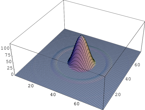
Figure 2.— Values of ${\cal A}_{ik}$ (as defined in the text) with fixed direction ${\bf e}_{i}$ at the center of the plot and direction ${\bf e}_{k}$ scanning a square of side $90^{\circ}$. We show the result for the COBE-DMR window function. The full width at half maximum of the plot is roughly $10^{\circ}$, of the same order as the resolution of the COBE-DMR detector. We can then expect the plotted ‘spike’ to select just one experimental pixel on the sky map, making the relation ${\cal A}_{ik}\approx\delta({\bf e}_{i}\!\cdot\!{\bf e}_{k}-1)$ a good approximation. Note that higher resolution experiments will yield a more peaked curve, although one would expect the goodness of the approximation to remain roughly the same.

Endowed now with the above regularization method, we present the term $\int\!\!\int{\rm d}\Omega_{5}{\rm d}\Omega_{6}E_{\rm S}^{\alpha}({}_{-},{\bf e}_{5},{\bf e}_{6})\xi({\bf e}_{5}\!\cdot\!{\bf e}_{6})$ in the following form

$$\int\!\!\int{\rm d}\Omega_{5}{\rm d}\Omega_{6}E_{\rm S}^{\alpha}({\bf e}_{4},{\bf e}_{5},{\bf e}_{6})\xi({\bf e}_{5}\!\cdot\!{\bf e}_{6})={{\cal D}\over 24\pi^{2}}\sum_{\alpha^{\prime}}\lambda^{\alpha}_{\alpha^{\prime}}\int\!\!\int\!\!\int{\rm d}\Omega_{i^{\prime}}{\rm d}\Omega_{j^{\prime}}{\rm d}\Omega_{k^{\prime}}\xi^{-1}({\bf e}_{4}\!\cdot\!{\bf e}_{i^{\prime}})\xi^{-1}({\bf e}_{j^{\prime}}\!\cdot\!{\bf e}_{k^{\prime}})R_{\rm S}^{\alpha^{\prime}}({\bf e}_{i^{\prime}},{\bf e}_{j^{\prime}},{\bf e}_{k^{\prime}})$$ (107)

with ${\cal D}\equiv{24\pi^{3}}[6+9{(2\pi)^{2}\over 3}(2\times 2\pi+4\pi{\cal A})]^{-1}$ where, as expected, the factor ${\cal A}$ appears explicitly. Now, we just replace the six terms with prefactor $9\xi\xi$ in the left hand side of Eq. (102) with Eq. (107) resulting in

$$\int\!\!\int\!\!\int \!\!{\rm d}\Omega_{4}{\rm d}\Omega_{5}{\rm d}\Omega_{6}\xi({\bf e}_{i}\!\cdot\!{\bf e}_{4})\xi({\bf e}_{j}\!\cdot\!{\bf e}_{5})\xi({\bf e}_{k}\!\cdot\!{\bf e}_{6})E_{\rm S}^{\alpha}({\bf e}_{4},{\bf e}_{5},{\bf e}_{6})$$

$$= {1\over 12}\sum_{\alpha^{\prime}}\lambda^{\alpha}_{\alpha^{\prime}}\Big{\{}R_{\rm S}^{\alpha^{\prime}}({\bf e}_{i},{\bf e}_{j},{\bf e}_{k})$$

$$- {{\cal D}\over 2\pi}\int\!\!\int{\rm d}\Omega_{j^{\prime}}{\rm d}\Omega_{k^{\prime}}\xi^{-1}({\bf e}_{j^{\prime}}\!\cdot\!{\bf e}_{k^{\prime}})\Big{[}R_{\rm S}^{\alpha^{\prime}}({\bf e}_{i},{\bf e}_{j^{\prime}},{\bf e}_{k^{\prime}})\xi({\bf e}_{j}\!\cdot\!{\bf e}_{k})+R_{\rm S}^{\alpha^{\prime}}({\bf e}_{j},{\bf e}_{j^{\prime}},{\bf e}_{k^{\prime}})\xi({\bf e}_{k}\!\cdot\!{\bf e}_{i})+R_{\rm S}^{\alpha^{\prime}}({\bf e}_{k},{\bf e}_{j^{\prime}},{\bf e}_{k^{\prime}})\xi({\bf e}_{i}\!\cdot\!{\bf e}_{j})\Big{]}\Big{\}}.$$

This contains just one appearance of $E^{\alpha}$; to get the weight function explicitly, we only need to multiply the equation by $\xi^{-1}({\bf e}_{i}\!\cdot\!{\bf e}_{1})\xi^{-1}({\bf e}_{j}\!\cdot\!{\bf e}_{2})\xi^{-1}({\bf e}_{k}\!\cdot\!{\bf e}_{3})$ and integrate over directions ${\bf e}_{i},{\bf e}_{j},{\bf e}_{k}$. Finally, we get the expression for $E_{\rm S}^{\alpha}$ in terms of the Lagrange multipliers $\lambda^{\alpha}$

$$E_{\rm S}^{\alpha}({\bf e}_{1},{\bf e}_{2},{\bf e}_{3})={1\over 12\times(2\pi)^{3}}\sum_{\alpha^{\prime}}\lambda^{\alpha}_{\alpha^{\prime}}\Big{\{}\int\!\!\int\!\!\int{\rm d}\Omega_{i}{\rm d}\Omega_{j}{\rm d}\Omega_{k}\xi^{-1}({\bf e}_{i}\!\cdot\!{\bf e}_{1})\xi^{-1}({\bf e}_{j}\!\cdot\!{\bf e}_{2})\xi^{-1}({\bf e}_{k}\!\cdot\!{\bf e}_{3})R_{\rm S}^{\alpha^{\prime}}({\bf e}_{i},{\bf e}_{j},{\bf e}_{k})$$

$$- {\cal D}\int\!\!\int\!\!\int{\rm d}\Omega_{i}{\rm d}\Omega_{j}{\rm d}\Omega_{k}R_{\rm S}^{\alpha^{\prime}}({\bf e}_{i},{\bf e}_{j},{\bf e}_{k})\xi^{-1}({\bf e}_{j}\!\cdot\!{\bf e}_{k})\Big{[}\xi^{-1}({\bf e}_{i}\!\cdot\!{\bf e}_{1})\xi^{-1}({\bf e}_{2}\!\cdot\!{\bf e}_{3})+\xi^{-1}({\bf e}_{i}\!\cdot\!{\bf e}_{2})\xi^{-1}({\bf e}_{3}\!\cdot\!{\bf e}_{1})+\xi^{-1}({\bf e}_{i}\!\cdot\!{\bf e}_{3})\xi^{-1}({\bf e}_{1}\!\cdot\!{\bf e}_{2})\Big{]}\Big{\}}$$

Reached this point, we have an explicit expression for $E_{\rm S}^{\alpha}$, but still dependent on the Lagrange multipliers. This equation is well defined as it contains the renormalized quantity ${\cal A}$. Within a particular experiment with a given resolution, the value ${\cal A}$ takes depends on what one means by two coincident directions. For example, for the COBE-DMR window-function specification (a Gaussian beam with dispersion $\sigma=3^{\circ}\hbox to0.0pt{\hss.}2$) this yields roughly ${\cal A}\approx 158.5$, including the quadrupole. It is not difficult to extend this to other scanning techniques. The previous equation is the analogue of our Eq. (39) corresponding to the second moment and also to Eq. (21) of (Heavens (1998)). In that article, a similar analysis is done but for the discretized CMB sky. Remark that no divergence appears in his case. Indeed, all relevant quantities are finite when evaluated for two directions pointing towards the same pixel. Our prefactor $\cal D$ corresponds to $3/(2+3N)$ in that paper, where $N$ represents the number of pixels in the map. Clearly, $N\to\infty$ when the pixel size goes to zero, as well as $\cal A\to\infty$ when the window function ${\cal W}_{\ell}\to 1$. At this intermediate step our corresponding expressions need not coincide because both depend on the particular regularization scheme used (be it discretization or usage of a window function). Despite appearances, we will show below that the final expression for the best unbiased estimator does not depend on these schemes. This cannot be inferred from Eq. (4.2) because we still need to remove the Lagrange multiplier. Unlike what was done in (Heavens (1998)), we now proceed further and express the weight function explicitly. Hence, we multiply both sides of Eq. (4.2) by $R_{\rm R}^{\alpha^{\prime\prime}}({\bf e}_{1},{\bf e}_{2},{\bf e}_{3})$, where $\alpha^{\prime\prime}\equiv{\tiny\{\begin{array}[]{ccc}\!\ell_{1}^{\prime\prime}\!&\!\ell_{2}^{\prime\prime}\!&\!\ell_{3}^{\prime\prime}\\ \!m_{1}^{\prime\prime}\!&\!m_{2}^{\prime\prime}\!&\!m_{3}^{\prime\prime}\end{array}\}}$, then integrate over directions ${\bf e}_{1}$, ${\bf e}_{2}$ and ${\bf e}_{3}$ and, upon using the constraint equation (98), we get

$$12\delta_{\rm S}^{\alpha\alpha^{\prime\prime}} = {1\over 6}{1\over{\cal C}_{\ell_{1}^{\prime\prime}}{\cal C}_{\ell_{2}^{\prime\prime}}{\cal C}_{\ell_{3}^{\prime\prime}}}\Big{\{}\Big{[}(-1)^{m_{1}^{\prime\prime}+m_{2}^{\prime\prime}+m_{3}^{\prime\prime}}\lambda^{\alpha}_{\left\{\!\tiny\begin{array}[]{ccc}\ell_{1}^{\prime\prime}\!&\!\ell_{2}^{\prime\prime}\!&\!\ell_{3}^{\prime\prime}\\ -m_{1}^{\prime\prime}\!&\!-m_{2}^{\prime\prime}\!&\!-m_{3}^{\prime\prime}\end{array}\!\right\}}+\lambda^{\alpha}_{\left\{\!\tiny\begin{array}[]{ccc}\ell_{1}^{\prime\prime}\!&\!\ell_{2}^{\prime\prime}\!&\!\ell_{3}^{\prime\prime}\\ m_{1}^{\prime\prime}\!&\!m_{2}^{\prime\prime}\!&\!m_{3}^{\prime\prime}\end{array}\!\right\}}\Big{]}+\mbox{\rm 5 additional permutations in index $\alpha^{\prime\prime}$}\Big{\}}$$ (114)

$$- {{\cal D}\over 3}\Biggl{\{}\Biggl{[}{\delta_{\ell_{1}^{\prime\prime}\ell_{2}^{\prime\prime}}\delta_{m_{1}^{\prime\prime}-m_{2}^{\prime\prime}}(-1)^{m_{2}^{\prime\prime}}\over{\cal C}_{\ell_{2}^{\prime\prime}}{\cal C}_{\ell_{3}^{\prime\prime}}}\sum_{\ell m}{(-1)^{m}\over{\cal C}_{\ell}}\Big{(}(-1)^{m_{3}^{\prime\prime}}\lambda^{\alpha}_{\left\{\!\tiny\begin{array}[]{ccc}\ell\!&\!\ell\!&\!\ell_{3}^{\prime\prime}\\ m\!&\!-m\!&\!-m_{3}^{\prime\prime}\end{array}\!\right\}}+\lambda^{\alpha}_{\left\{\!\tiny\begin{array}[]{ccc}\ell\!&\!\ell\!&\!\ell_{3}^{\prime\prime}\\ -m\!&\!m\!&\!m_{3}^{\prime\prime}\end{array}\!\right\}}+(-1)^{m_{3}^{\prime\prime}}\lambda^{\alpha}_{\left\{\!\tiny\begin{array}[]{ccc}\ell_{3}^{\prime\prime}\!&\!\ell\!&\!\ell\\ -m_{3}^{\prime\prime}\!&\!m\!&\!-m\end{array}\!\right\}}+\lambda^{\alpha}_{\left\{\!\tiny\begin{array}[]{ccc}\ell_{3}^{\prime\prime}\!&\!\ell\!&\!\ell\\ m_{3}^{\prime\prime}\!&\!-m\!&\!m\end{array}\!\right\}}$$ (123)

$$+ (-1)^{m_{3}^{\prime\prime}}\lambda^{\alpha}_{\left\{\!\tiny\begin{array}[]{ccc}\ell\!&\!\ell_{3}^{\prime\prime}\!&\!\ell\\ m\!&\!-m_{3}^{\prime\prime}\!&\!-m\end{array}\!\right\}}+\lambda^{\alpha}_{\left\{\!\tiny\begin{array}[]{ccc}\ell\!&\!\ell_{3}^{\prime\prime}\!&\!\ell\\ -m\!&\!m_{3}^{\prime\prime}\!&\!m\end{array}\!\right\}}\Big{)}\Biggr{]}+{\tiny\Big{[}\begin{array}[]{c}1\to 2\\ 2\to 3\\ 3\to 1\end{array}\Big{]}}+{\tiny\Big{[}\begin{array}[]{c}1\to 3\\ 2\to 1\\ 3\to 2\end{array}\Big{]}}\Biggr{\}}.$$ (134)

Eq. (114) is the final algebraic equation that the multipliers must satisfy. For fixed $\alpha$, a natural way to proceed would be to get an explicit expression for $\lambda^{\alpha}_{\alpha^{\prime}}$. Another way to solve the problem goes on a line analogous to the case of the two-point correlators: we just need to identify the complicated combination of Lagrange multipliers in the right hand side of Eq. (114) with the one in the right hand side of Eq. (4.2) [or, equivalently, Eq. (4.2)]. In order to do that, we now multiply both sides of Eq. (114) by $R_{\rm R}^{\alpha^{\prime\prime}}({\bf e}_{i},{\bf e}_{j},{\bf e}_{k})$, perform the six sums over the indices in ${\alpha^{\prime\prime}}$ and we end up with

$$R_{\rm S}^{\alpha}({\bf e}_{i},{\bf e}_{j},{\bf e}_{k}){\cal C}_{\ell_{1}}{\cal C}_{\ell_{2}}{\cal C}_{\ell_{3}}=\sum_{\alpha^{\prime\prime}}R_{\rm R}^{\alpha^{\prime\prime}}({\bf e}_{i},{\bf e}_{j},{\bf e}_{k}){\cal C}_{\ell_{1}^{\prime\prime}}{\cal C}_{\ell_{2}^{\prime\prime}}{\cal C}_{\ell_{3}^{\prime\prime}}\delta_{\rm S}^{\alpha\alpha^{\prime\prime}}$$ (147)

$$= {1\over 12}\sum_{\alpha^{\prime}}\lambda^{\alpha}_{\alpha^{\prime}}R_{\rm S}^{\alpha^{\prime}}({\bf e}_{i},{\bf e}_{j},{\bf e}_{k})-{{\cal D}\over 36}\sum_{LM}\sum_{\ell m}{(-1)^{M}\over{\cal C}_{L}}\Big{[}Y_{\ell}^{m}({\bf e}_{i})\xi({\bf e}_{j}\!\cdot\!{\bf e}_{k})+Y_{\ell}^{m}({\bf e}_{j})\xi({\bf e}_{k}\!\cdot\!{\bf e}_{i})+Y_{\ell}^{m}({\bf e}_{k})\xi({\bf e}_{i}\!\cdot\!{\bf e}_{j})\Big{]}$$

$$\times \Big{[}\lambda^{\alpha}_{\left\{\!\tiny\begin{array}[]{ccc}\ell\!&\!L\!&\!L\\ m\!&\!M\!&\!-M\end{array}\!\right\}}+(-1)^{m}\lambda^{\alpha}_{\left\{\!\tiny\begin{array}[]{ccc}\ell\!&\!L\!&\!L\\ -m\!&\!-M\!&\!M\end{array}\!\right\}}+\lambda^{\alpha}_{\left\{\!\tiny\begin{array}[]{ccc}L\!&\!\ell\!&\!L\\ -M\!&\!m\!&\!M\end{array}\!\right\}}+(-1)^{m}\lambda^{\alpha}_{\left\{\!\tiny\begin{array}[]{ccc}L\!&\!\ell\!&\!L\\ M\!&\!-m\!&\!-M\end{array}\!\right\}}+\lambda^{\alpha}_{\left\{\!\tiny\begin{array}[]{ccc}L\!&\!L\!&\!\ell\\ M\!&\!-M\!&\!m\end{array}\!\right\}}+(-1)^{m}\lambda^{\alpha}_{\left\{\!\tiny\begin{array}[]{ccc}L\!&\!L\!&\!\ell\\ -M\!&\!M\!&\!-m\end{array}\!\right\}}\Big{]}.$$

This is the equivalent of Eq. (40). The aim now is to show that the combination of Lagrange multipliers in the right hand side of the previous equation is precisely the one which appears in the right hand side of Eq. (4.2). In the latter, let us express both $R_{\rm S}^{\alpha^{\prime}}$ and $\xi^{-1}$ in the second term in the right hand side in terms of spherical harmonics. After some algebra we get

$$\int\!\!\int\!\!\int \!\!{\rm d}\Omega_{4}{\rm d}\Omega_{5}{\rm d}\Omega_{6}\xi({\bf e}_{i}\!\cdot\!{\bf e}_{4})\xi({\bf e}_{j}\!\cdot\!{\bf e}_{5})\xi({\bf e}_{k}\!\cdot\!{\bf e}_{6})E_{\rm S}^{\alpha}({\bf e}_{4},{\bf e}_{5},{\bf e}_{6})$$ (160)

$$= {1\over 12}\sum_{\alpha^{\prime}}\lambda^{\alpha}_{\alpha^{\prime}}R_{\rm S}^{\alpha^{\prime}}({\bf e}_{i},{\bf e}_{j},{\bf e}_{k})-{{\cal D}\over 36}\sum_{LM}\sum_{\ell m}{(-1)^{M}\over{\cal C}_{L}}\Big{[}Y_{\ell}^{m}({\bf e}_{i})\xi({\bf e}_{j}\!\cdot\!{\bf e}_{k})+Y_{\ell}^{m}({\bf e}_{j})\xi({\bf e}_{k}\!\cdot\!{\bf e}_{i})+Y_{\ell}^{m}({\bf e}_{k})\xi({\bf e}_{i}\!\cdot\!{\bf e}_{j})\Big{]}$$

$$\times \Big{[}\lambda^{\alpha}_{\left\{\!\tiny\begin{array}[]{ccc}\ell\!&\!L\!&\!L\\ m\!&\!M\!&\!-M\end{array}\!\right\}}+(-1)^{m}\lambda^{\alpha}_{\left\{\!\tiny\begin{array}[]{ccc}\ell\!&\!L\!&\!L\\ -m\!&\!-M\!&\!M\end{array}\!\right\}}+\lambda^{\alpha}_{\left\{\!\tiny\begin{array}[]{ccc}L\!&\!\ell\!&\!L\\ -M\!&\!m\!&\!M\end{array}\!\right\}}+(-1)^{m}\lambda^{\alpha}_{\left\{\!\tiny\begin{array}[]{ccc}L\!&\!\ell\!&\!L\\ M\!&\!-m\!&\!-M\end{array}\!\right\}}+\lambda^{\alpha}_{\left\{\!\tiny\begin{array}[]{ccc}L\!&\!L\!&\!\ell\\ M\!&\!-M\!&\!m\end{array}\!\right\}}+(-1)^{m}\lambda^{\alpha}_{\left\{\!\tiny\begin{array}[]{ccc}L\!&\!L\!&\!\ell\\ -M\!&\!M\!&\!-m\end{array}\!\right\}}\Big{]},$$

which, as advertised, yields the same combination of Lagrange multipliers of Eq. (147). Then, putting the last two equations together, multiplying by $\xi^{-1}$ and integrating three times, we finally get the weight function associated to the best unbiased estimator

$$E_{\rm S,Best}^{\alpha}({\bf e}_{i},{\bf e}_{j},{\bf e}_{k})=R_{\rm S}^{\alpha}({\bf e}_{i},{\bf e}_{j},{\bf e}_{k}),$$ (161)

which implies that the best unbiased estimator itself is given by

$${\cal E}_{\rm Best}({\cal B}^{\alpha})=\frac{1}{2}\Big{(}a_{\ell_{1}}^{m_{1}}a_{\ell_{2}}^{m_{2}}a_{\ell_{3}}^{m_{3}}+a_{\ell_{1}}^{m_{1}*}a_{\ell_{2}}^{m_{2}*}a_{\ell_{3}}^{m_{3}*}\Big{)}.$$ (162)

This is the final answer and it is a new result. Let us make a few remarks. Firstly, this does not depend on ${\cal A}$ which shows that Eq. (162) is independent of the regularization scheme used. Secondly, Luo (1994) used the following complex unbiased estimator: ${\cal E}({\cal B}^{\alpha})=a_{\ell_{1}}^{m_{1}}a_{\ell_{2}}^{m_{2}}a_{\ell_{3}}^{m_{3}}$, although he did not claim it to be the best one. Thirdly, as for the two-point correlators, one cannot use Eq. (162) in order to infer ${\cal E}_{\rm Best}({\cal C}_{\ell_{1}\ell_{2}\ell_{2}})$. Indeed, promoting the equation

$$\bigl{\langle}a_{\ell_{1}}^{m_{1}}a_{\ell_{2}}^{m_{2}}a_{\ell_{3}}^{m_{3}}\bigr{\rangle}=\left(\begin{array}[]{ccc}\ell_{1}&\ell_{2}&\ell_{3}\\ m_{1}&m_{2}&m_{3}\end{array}\right){\cal C}_{\ell_{1}\ell_{2}\ell_{3}},$$ (163)

valid for the mean values of the estimators, to the following equation

$${\cal E}_{\rm Best}({\cal B}^{\alpha})=\frac{1}{2}\Big{(}a_{\ell_{1}}^{m_{1}}a_{\ell_{2}}^{m_{2}}a_{\ell_{3}}^{m_{3}}+a_{\ell_{1}}^{m_{1}*}a_{\ell_{2}}^{m_{2}*}a_{\ell_{3}}^{m_{3}*}\Big{)}={\cal E}_{\rm Best}({\cal C}_{\ell_{1}\ell_{2}\ell_{3}})\left(\begin{array}[]{ccc}\ell_{1}&\ell_{2}&\ell_{3}\\ m_{1}&m_{2}&m_{3}\end{array}\right)\quad\mbox{(false)},$$ (164)

valid for the estimators themselves, is an unjustified step. If, nevertheless, we used this false relation we would get

$${\cal E}_{\rm Best}({\cal B}^{\alpha})=\left(\begin{array}[]{ccc}\ell_{1}&\ell_{2}&\ell_{3}\\ m_{1}&m_{2}&m_{3}\end{array}\right)\sum_{m_{1}^{\prime}m_{2}^{\prime}m_{3}^{\prime}}\left(\begin{array}[]{ccc}\ell_{1}&\ell_{2}&\ell_{3}\\ m_{1}^{\prime}&m_{2}^{\prime}&m_{3}^{\prime}\end{array}\right)a_{\ell_{1}}^{m_{1}^{\prime}}a_{\ell_{2}}^{m_{2}^{\prime}}a_{\ell_{3}}^{m_{3}^{\prime}}\quad\mbox{(false)},$$ (165)

which cannot be cast into $\frac{1}{2}\Big{(}a_{\ell_{1}}^{m_{1}}a_{\ell_{2}}^{m_{2}}a_{\ell_{3}}^{m_{3}}+a_{\ell_{1}}^{m_{1}*}a_{\ell_{2}}^{m_{2}*}a_{\ell_{3}}^{m_{3}*}\Big{)}$. So, like for the two-point correlators, we see that one cannot infer the ${\cal E}_{\rm Best}({\cal B}^{\alpha})$ from ${\cal E}_{\rm Best}({\cal C}_{\ell_{1}\ell_{2}\ell_{3}})$ and vice versa.

Endowed now with the best unbiased estimator, one can compute its variance squared, the ‘third-moment cosmic variance’, which reads

$$\sigma^{2}_{{\cal E}_{\rm Best}({\cal B}^{\alpha})} = \frac{1}{2}\Big{\{}{\cal C}_{\ell_{1}}{\cal C}_{\ell_{2}}{\cal C}_{\ell_{3}}\Big{[}1+\delta_{m_{1}0}\delta_{m_{2}0}\delta_{m_{3}0}\Big{]}+{\cal C}_{\ell_{1}}^{3}\delta_{\ell_{1}\ell_{2}\ell_{3}}\Big{[}8\delta_{m_{1}0}\delta_{m_{2}0}\delta_{m_{3}0}+2(\delta_{m_{1}m_{3}}+\delta_{m_{1}-m_{3}})(\delta_{m_{1}m_{2}}+\delta_{m_{1}-m_{2}})\Big{]}$$ (166)

$$+ {\cal C}_{\ell_{1}}{\cal C}_{\ell_{2}}^{2}\delta_{\ell_{2}\ell_{3}}\Big{[}2\delta_{m_{1}0}\delta_{m_{2}-m_{3}}+\delta_{m_{2}m_{3}}+\delta_{m_{2}-m_{3}}\Big{]}+{\cal C}_{\ell_{2}}{\cal C}_{\ell_{3}}^{2}\delta_{\ell_{3}\ell_{1}}\Big{[}2\delta_{m_{2}0}\delta_{m_{3}-m_{1}}+\delta_{m_{3}m_{1}}+\delta_{m_{3}-m_{1}}\Big{]}$$

$$+ {\cal C}_{\ell_{3}}{\cal C}_{\ell_{1}}^{2}\delta_{\ell_{1}\ell_{2}}\Big{[}2\delta_{m_{3}0}\delta_{m_{1}-m_{2}}+\delta_{m_{1}m_{2}}+\delta_{m_{1}-m_{2}}\Big{]}\Big{\}}.$$

For example, from this we can now compute the cosmic variance for the third-moment estimator ${\cal E}_{\rm Best}({\cal B}^{\beta})$ with $\beta\equiv{\tiny\{\begin{array}[]{ccc}\!\ell\!&\!\ell\!&\!\ell\\ \!m\!&\!m\!&\!-2m\end{array}\}}$ where $\ell=\mbox{even}$ and $m\neq 0$. This particular case is often treated in the literature, see e.g. (Luo 1994, Heavens 1998). We find $\sigma^{2}_{{\cal E}_{\rm Best}({\cal B}^{\beta})}={\cal C}^{3}_{\ell}$ whereas the variance of the estimator used in (Luo 1994) yields $\sigma^{2}_{{\cal E}({\cal B}^{\beta})}=2\,{\cal C}^{3}_{\ell}$. Another example comes from taking $\gamma\equiv{\tiny\{\begin{array}[]{ccc}\!\ell\!&\!\ell\!&\!\ell\\ \!m_{1}\!&\!m_{2}\!&\!m_{3}\end{array}\}}$ where $|m_{i}|\neq|m_{j}|$ for any $i,j$. With this choice we get $\sigma^{2}_{{\cal E}_{\rm Best}({\cal B}^{\gamma})}={\cal C}^{3}_{\ell}/2$ whereas Luo (1994) obtains $\sigma^{2}_{{\cal E}({\cal B}^{\gamma})}={\cal C}^{3}_{\ell}$. Note that in both examples the results differ by a 1/2 factor. This can be traced back to the form of the best estimator in Eq. (162). The variance computed in (Luo 1994) is consistent with his choice of the estimator. However, unlike what is stated in that paper, this variance does not deserve the name ‘cosmic’ because, as we saw above, this estimator is not the best one. As expected, the variance of the best estimator is smaller than the variance computed in his article. Since we have now the correct expression for the cosmic variance, its numerical value should be re-estimated. To be specific, let us take $\beta\equiv{\tiny\{\begin{array}[]{ccc}\!2\!&\!2\!&\!2\\ \!1\!&\!1\!&\!-2\end{array}\}}$. The cosmic variance is then $\sigma_{{\cal E}_{\rm Best}({\cal B}^{\beta})}={\cal C}^{3/2}_{2}=(4\pi/5)^{3/2}Q_{\rm rms-PS}^{3}/T_{0}^{3}\approx 1.3\times 10^{-15}$ where we used $T_{0}=2.7$ K and $Q_{\rm rms-PS}=18.7\mu$K (Bunn & White (1997)). Although this figure is close to Luo’s result ($1.4\times 10^{-15}$) cited after equation (32) in (Heavens 1998), this does not imply that the two variances are not different by a factor 1/2, as we have just seen. This might probably be due to a difference in the quadrupole normalizations.

5. Conclusions

Optimized analyses of CMB datasets involve the use of appropriate methods in order to reduce the various uncertainties. In particular, the theoretical error bars due to the cosmic variance can be minimized by working with the method of the best unbiased estimators. In this article, we have applied this technique for the study of CMB non-Gaussian features. These are often characterized by means of the third moment for the $a^{m}_{\ell}$’s or by the angular bispectrum ${\cal C}_{\ell_{1}\ell_{2}\ell_{3}}$. We have found the best unbiased estimators in both cases. These are the quantities that should be used in future data analyses and would be important for upcoming megapixel experiments (Tegmark (1997); Borrill (1999)) like MAP and Planck Surveyor. In addition to this, we have displayed both the angular bispectrum and the third moment cosmic variances, the smallest possible uncertainties attached to the bispectrum and the third moment, which would be present in any ideal experiment when all other sources of noise have been removed.

6. Appendix: The inverse two-point correlation function

In this Appendix, we derive the exact expression of the inverse of the two-point correlation function $\xi^{-1}$, defined according to

$$\int{\rm d}\Omega_{j}\xi({\bf e}_{i}\!\cdot\!{\bf e}_{j})\xi^{-1}({\bf e}_{j}\!\cdot\!{\bf e}_{k})\equiv\delta({\bf e}_{i}\!\cdot\!{\bf e}_{k}-1).$$ (167)

As usual, one expands the two-point correlation function on the basis of the Legendre polynomials

$$\xi({\bf e}_{i}\!\cdot\!{\bf e}_{j})=\sum_{\ell}{2\ell+1\over 4\pi}{\cal C}_{\ell}P_{\ell}({\bf e}_{i}\!\cdot\!{\bf e}_{j}).$$ (168)

In general, $\xi^{-1}$ can be expanded on the spherical harmonics basis as follows

$$\xi^{-1}({\bf e}_{i}\!\cdot\!{\bf e}_{j})=\sum_{\ell m}\sum_{\ell^{\prime}m^{\prime}}b_{\ell\ell^{\prime}mm^{\prime}}Y_{\ell}^{m}({\bf e}_{i})Y_{\ell^{\prime}}^{m^{\prime}*}({\bf e}_{j}).$$ (169)

Our aim now is to determine the coefficients $b_{\ell\ell^{\prime}mm^{\prime}}$. Using Eqns. (168) and (169), the completeness relation for the Legendre polynomials together with the addition theorem of spherical harmonics in Eq. (167), one gets

$$\sum_{\ell m}\sum_{\ell^{\prime}m^{\prime}}{\cal C}_{\ell}b_{\ell\ell^{\prime}mm^{\prime}}Y_{\ell}^{m}({\bf e}_{i})Y_{\ell^{\prime}}^{m^{\prime}*}({\bf e}_{k})=\sum_{\ell^{\prime\prime}}(\ell^{\prime\prime}+\frac{1}{2})P_{\ell^{\prime\prime}}({\bf e}_{i}\cdot{\bf e}_{k}).$$ (170)

The coefficients $b_{\ell\ell^{\prime}mm^{\prime}}$ are easy to read off and one obtains

$$b_{\ell\ell^{\prime}mm^{\prime}}=\frac{2\pi}{{\cal C}_{\ell}}\delta_{\ell\ell^{\prime}}\delta_{mm^{\prime}},$$ (171)

from which one deduces

$$\xi^{-1}({\bf e}_{i}\!\cdot\!{\bf e}_{j})=\sum_{\ell}\frac{\ell+1/2}{{\cal C}_{\ell}}P_{\ell}({\bf e}_{i}\cdot{\bf e}_{j}).$$ (172)

This is the expression used in the main text.

References

• Albrecht & Steinhardt (1982) Albrecht, A. & Steinhardt, P. J. 1982, Phys. Rev. Lett. 48, 1220.
• Avelino et al. (1998) Avelino, P .P. et al. 1998, Astrophys. J., 507, L101.
• (3) Banday, A. J., Zaroubi, S. & Górski, K. M, astro-ph/9908070.
• Bardeen et al. (1983) Bardeen, J. M., Steinhardt, P. J. & Turner, M. S. 1983, Phys. Rev. D 28, 679.
• Bernardeau (1997) Bernardeau, F. 1997, Astronomy and Astrophysics, 324, 15.
• Bond & Efstathiou (1987) Bond, J. R. & Efstathiou, G. 1987, MNRAS 226, 655.
• Borrill (1999) Borrill, J. 1999, astro-ph/9911389.
• Bouchet & Gispert (1999) Bouchet, F. & Gispert, R. 1999, astro-ph/9903176.
• Bouchet et al. (1988) Bouchet, F. R., Bennett, D. P. & Stebbins, A. 1988, Nature 335, 410.
• Brandenberger & Hill (1986) Brandenberger, R. H. & Hill, C. T. 1986, Phys. Lett. B 179, 30.
• Bromley & Tegmark (1999) Bromley, B. & Tegmark, M. Astrophys. J. Lett. in press (astro-ph/9904254).
• Bunn & Scott (1999) Bunn, E. & Scott, D. 1999, astro-ph/9906044.
• Bunn & White (1997) Bunn, E. F. & White, M. 1997, Astrophys. J. 480, 6.
• Coles (1989) Coles, P. 1989, MNRAS, 234, 509.
• Contaldi et al. (1999) Contaldi, C. R., Bean, R. & Magueijo, J. 1999, Phys. Lett. B 468, 189.
• Cooray & Hu (1999) Cooray, A. & Hu, W. 1999, astro-ph/9910397.
• Falk et al. (1993) Falk, T., Rangarajan, R. & Srednicki, M. 1993, Astrophys. J. 403, L1.
• Ferreira & Magueijo (1997) Ferreira, P. & Magueijo, J. 1997, Phys. Rev. D 55, 3358.
• Ferreira et al. (1998) Ferreira, P. G., Magueijo, J. & Górksi, K. M. 1998, Astrophys. J. 503, L1.
• Gangui (1994) Gangui, A. 1994, Phys. Rev. D. 50, 3684.
• Gangui et al. (1994) Gangui, A., Lucchin, F., Matarrese, S. & Mollerach, S. 1994, Astrophys. J. 430, 447.
• Gangui & Martin (2000) Gangui, A. & Martin, J. 2000, Mon. Not. R. Astron. Soc. 313, 323. astro-ph/9908009.
• Gangui & Mollerach (1996) Gangui, A. & Mollerach, S. 1996, Phys. Rev. D 54, 4750.
• Gangui & Perivolaropoulos (1995) Gangui, A. & Perivolaropoulos, L. 1995, Astrophys. J. 447, 1.
• Goldberg & Spergel (1999) Goldberg, D. M. & Spergel, D. N. 1999, Phys. Rev D 59, 103002.
• Górski (1994) Górksi, K. M. 1994, Astrophys. J. 430, L85.
• Gott et al. (1990) Gott, J. R. et al. 1990, Astrophys. J. 352, 1.
• Grishchuk & Sidorov (1990) Grishchuk, L. P. & Sidorov, Y. 1990, Phys. Rev. D 42, 3413.
• Grishchuk (1993) Grishchuk, L. P. 1993, Phys. Rev. D 48, 3513.
• Grishchuk & Martin (1997) Grishchuk, L. P. & Martin, J. 1997, Phys. Rev. D 56, 1924.
• Guth (1981) Guth, A. 1981, Phys. Rev. D 23, 347.
• Halliwell (1989) Halliwell, J. J. 1989, in Quantum Cosmology and Baby Universes, Proceedings of the 1989 Jerusalem Winter School for Theoretical Physics, Eds. Coleman S. et al., World Scientific, Singapore.
• Hawking (1982) Hawking, S. W. 1982, Phys. Lett. B 115, 295.
• Heavens (1998) Heavens, A. 1998, MNRAS 299, 805.
• Heavens & Sheth (1999) Heavens, A. & Sheth, R. 1999, astro-ph/9904307.
• Hinshaw et al. (1994) Hinshaw, G. et al. 1994, Astrophys. J. 431, 431.
• Hinshaw et al. (1995) Hinshaw, G. et al. 1995, Astrophys. J. 446, L67.
• Hobson et al. (1998) Hobson, M. et al. 1998, astro-ph/9810200.
• Knox (1999) Knox, L. 1999, astro-ph/9902046.
• Kogut et al. (1995) Kogut, A. et al. 1995, Astrophys. J. 439, L29.
• Kogut et al. (1996) Kogut, A. et al. 1996, Astrophys. J. 464, L29.
• (42) Linde, A. 1983, Phys. Lett. B 108, 389.
• (43) Linde, A. 1983, Phys. Lett. B 129, 177.
• Linde & Mukhanov (1997) Linde, A. & Mukhanov, V. 1997, Phys. Rev. D 56, 535.
• Luo (1994) Luo, X. 1994, Astrophys. J. 427, L71.
• Luo & Schramm (1993) Luo, X. & Schramm, D. N. 1993, Phys. Rev. Lett. 71, 1124.
• Magueijo (1999) Magueijo, J. 1999, astro-ph/9911334.
• Martin et al. (1999) Martin, J., Riazuelo, A. & Sakellariadou, M. 1999, astro-ph/9904167, to appear in Phys. Rev. D.
• Martin & Schwarz (1998) Martin, J. & Schwarz, D. J. 1998, Phys. Rev. D 57, 3302.
• Martin & Schwarz (1999) Martin, J. & Schwarz, D. J. 1999, astro-ph/9911225.
• Mollerach et al. (1995) Mollerach, S., Gangui, A., Lucchin, F. & Matarrese, S. 1995, Astrophys. J. 453, 1.
• Mukhanov & Chibisov (1981) Mukhanov, V. F. & Chibisov, G. 1981, JETP lett. 33, 532.
• Mukhanov et al. (1992) Mukhanov, V. F., Feldman, H. A. & Brandenberger, R. H. 1992, Phys. Rep. 215, 203.
• Munshi et al. (1995) Munshi, D., Souradeep, T. & Starobinsky, A. A. 1995, Astrophys. J. 454, 552.
• Pando et al. (1998) Pando, J., Vallas-Gabaud, D. & Fang, L. 1998, Phys. Rev. Lett. 79, 1611.
• Popa (1998) Popa, L. 1998, astro-ph/9806086.
• Scaramella & Vittorio (1991) Scaramella, R. & Vittorio, N. 1991, Astrophys. J. 375, 439.
• Scott (1999) Scott, D. 1999, astro-ph/9912038.
• Smoot (1999) Smoot, G. et al. 1994, Astrophys. J. 437, 1.
• Spergel & Goldberg (1999) Spergel, D. N & Goldberg, D. M. 1999, Phys. Rev. D 59, 103001.
• Srednicki (1993) Srednicki, M. 1993, Astrophys. J. 416, L1.
• Starobinsky (1982) Starobinsky, A. A. 1982, Phys. Lett. B 117, 175.
• Tegmark (1997) Tegmark, M. 1997, Astrophys. J. 480, L87.
• Tegmark et al. (1999) Tegmark, M. et al. 1999, astro-ph/9905257.
• Wang & Kamionkowski (2000) Wang, L. & Kamionkowski, M. 2000, PRD, astro-ph/9907431.
• White & Srednicki (1995) White, M. & Srednicki, M. 1995, Astrophys. J. 443, 6.
• Winitzki (1998) Winitzki, S. 1998, astro-ph/9806105.
• Winitzki & Kosowsky (1998) Winitzki, S. & Kosowsky, A. 1998, New Astronomy 3, 75.
• Zaldarriaga (1999) Zaldarriaga, M. 1999, astro-ph/9910498.